Complementarity Between Sentinel-1 and Landsat 8 Imagery for Built-Up Mapping in Sub-Saharan Africa

RESEARCH OUTPUTS / RÉSULTATS DE RECHERCHE

Author(s) - Auteur(s) :

Publication date - Date de publication :

Permanent link - Permalien :

Rights / License - Licence de droit d’auteur :

Bibliothèque Universitaire Moretus Plantin

researchportal.unamur.be

University of Namur

Complementarity Between Sentinel-1 and Landsat 8 Imagery for Built-Up Mapping in

Sub-Saharan Africa

Forget, Yann; Shimoni, Michal; Gilbert, Marius; Linard, Catherine

Early version, also known as pre-print Link to publication

Citation for pulished version (HARVARD):

Forget, Y, Shimoni, M, Gilbert, M & Linard, C 2018, 'Complementarity Between Sentinel-1 and Landsat 8 Imagery for Built-Up Mapping in Sub-Saharan Africa', Polymer Preprints.

https://doi.org/10.20944/preprints201810.0695.v1

General rights

Copyright and moral rights for the publications made accessible in the public portal are retained by the authors and/or other copyright owners and it is a condition of accessing publications that users recognise and abide by the legal requirements associated with these rights. • Users may download and print one copy of any publication from the public portal for the purpose of private study or research. • You may not further distribute the material or use it for any profit-making activity or commercial gain

• You may freely distribute the URL identifying the publication in the public portal ? Take down policy

If you believe that this document breaches copyright please contact us providing details, and we will remove access to the work immediately and investigate your claim.

Complementarity Between Sentinel-1 and Landsat 8

Imagery for Built-Up Mapping in Sub-Saharan Africa

Yann Forget1 *, Michal Shimoni2 , Marius Gilbert1 and Catherine Linard3

1 _{Spatial Epidemiology Lab (SpELL), Université Libre de Bruxelles, Brussels, Belgium.} 2 _{Signal and Image Centre, Belgian Royal Military Academy (SIC-RMA), Brussels, Belgium.} 3 _{Department of Geography, University of Namur, Namur, Belgium.}

* Correspondence: yannforget@mailbox.org

Abstract:The rapid urbanization that takes place in developing regions such as Sub-Saharan Africa is associated with a large range of environmental and social issues. In this context, remote sensing is essential to provide accurate and up-to-date spatial information to support risk assessment and decision making. However, mapping urban areas remains a challenge because of their heterogeneity, especially in developing regions where the highest rates of misclassification are observed. Nevertheless, urban areas located in arid climates — which are among the most vulnerables to anthropogenic impacts, suffer from the spectral confusion occurring between built-up and bare soil areas when using optical imagery. Today, the increasing availability of satellite imagery from multiple sensors allow to tackle the aforementioned issues by combining optical data with Synthetic Aperture Radar (SAR). In this paper, we assess the complementarity of the Landsat 8 and Sentinel-1 sensors to map built-up areas in twelve Sub-Saharan African urban areas, using a pixel-level supervised classification based on the Random Forest classifier. We make use of textural information extracted from SAR backscattering data in order to reduce the speckle noise and to introduce contextual information at the pixel level. Results suggest that combining both optical and SAR features consistently improves classification performances, mainly by enhancing the differentiation between built-up and bare lands. However, the fusion was less beneficial in mountainous case studies, suggesting that including features derived from a Digital Elevation Model (DEM) could improve the reliability of the proposed approach. As suggested by previous studies, combining features computed from both VV and VH polarizations consistently led to better classification performances. On the contrary, introducing textures computed from different spatial scales did not improve the classification performances.

Keywords:Urban Remote Sensing; Sentinel-1; Landsat 8; Built-Up; Data Fusion; Texture; Africa

1. Introduction

Urbanization is a worldwide process associated with a wide range of environmental and human health issues [1,2]. In Africa, the urban population is predicted to triple between 2010 and 2050, threatening both social and environmental sustainability [3]. Monitoring built-up areas in developing regions such as Sub-Saharan Africa is therefore crucial to understand, predict, and mitigate the risks associated with such a rapid urbanization [4]. In this context, remote sensing plays a major role by providing accurate spatial information on built-up areas at a relatively low cost [5,6]. However, because of the heterogeneity of urban areas in terms of spatial structure and materials, mapping built-up with medium resolution optical imagery remains challenging. In medium spatial resolution imagery (10-50 meters), urban pixels are made of a combination of several elements — such as buildings, roads, trees or bare soil. Furthermore, the spectral characteristics and the spatial distribution of these objects differ across a given urban area. High differences are also observed among the cities of the world because of socioeconomic, cultural, historical and environmental variations [7–9]. Developing regions are the most concerned with the urbanization-related risks, — but previous studies have shown that they

also suffer from lower accuracies in global built-up maps [10], because of a high urban heterogeneity coupled with a lack of reference datasets to support the training and the validation of the classification models.

Likewise, urban areas located in arid and semi-arid climates are among the most vulnerables to anthropogenic impacts. Despite the fact that about one third of the global land surface is characterized by an arid or semi-arid climate according to the Köppen-Geiger classification [11,12], they also suffer from low accuracies when it comes to built-up mapping. Due to their overlapping spectral signatures, the differentiation between bare land and built-up in arid and semi-arid environments has proven to be one of the main challenge associated with optical sensors in urban remote sensing. Previous studies have shown that conventional spectral indices — such as the normalized difference built-up index (NDBI), the normalized difference bareness index (NDBal), or the urban index (UI), are not reliable to differentiate built-up areas from bare land in arid regions [13,14]. As a result, new approaches based on object-oriented classification or linear spectral mixture analysis have been proposed [13,15]. New spectral indices have also been specifically developed to tackle the issue, such as the normalized bare land index (NBLI) [16]. Likewise, the dry built-up index (DBI) and the dry bare-soil index (DBSI) provide a better separation between bare soil and built-up in arid regions by making use of the blue and thermal bands of Landsat 8 [14]. Approaches based on the thresholding of spectral indices do not require any training dataset and benefit from a low computational cost. However, as stated by their authors, their reliability highly depends on the landscape and the climate of the study area. For instance, the DBSI is not considered suitable in humid regions or in urban areas surrounded by vegetation [14].

Because of the aforementioned issues, the idea of combining optical data with complementary sensors such as Synthetic Aperture Radar (SAR) recently gained momentum. SAR has the advantages of providing high resolution imagery independently from daylight, clouds, or weather conditions. The C-band of the European Remote-Sensing Satellite 1 and 2 (ERS-1/2) has been widely used to monitor urban areas [17]. In contrast to optical sensors, SAR is sensitive to the roughness of the terrain — and thus is able to better differentiate between bare soil and built-up [18]. Previous studies have shown that the combined use of optical and SAR data can significantly improves the accuracy of a land cover classification [19–21]. However, classifying data provided by different sensors is not straightforward and there is no consensus among the remote sensing community regarding the best fusion approach. Conventional parametric classifiers which concatenate signals from different sensors into one vector have been shown to be inefficient in modeling multi-sensor data distributions, therefore most of the methods rely on machine learning classifiers that do not make any assumption regarding the data distribution [22]. Fusion can occur at four different levels: (1) at the signal level, (2) at the pixel level — by concatenating data from multiple sensors into one stacked vector [23–26], (3) at the feature level in the context of an object-based classification that makes use of image segmentation techniques [27], or (4) at the decision level, for instance by merging several single-source classifiers using neural networks or support vector machines [19,28–30].

Previous studies have reported that pixel-level fusion approaches are inappropriate because of the lack of information about the spatial context of a given pixel and the speckle noise inherent to SAR data [22,25,31]. The extraction of textural features from SAR backscattering partially solves the aforementioned issues [25,26], for instance by computing the grey level co-occurrence matrix (GLCM) texture features [32,33]. However, there is no consensus on which features are the most relevant in the context of a combined use with optical data, or on the optimal size of the moving window used to compute the GLCM.

In this paper, we investigate the combined use of Landsat 8 and Sentinel-1 imagery to detect built-up in twelve Sub-Saharan African case studies characterized by various climates, landscapes and population patterns. We assess the complementarity of optical and SAR data in the context of a pixel-level supervised classification based on the extraction of 18 GLCM texture features, with several window sizes and from the two polarizations available with Sentinel-1 — VV and VH.

2. Materials and methods 2.1. Case studies

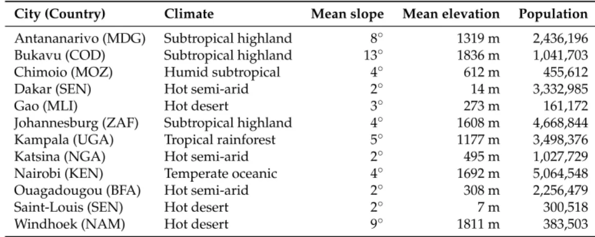
Table 1.Climate, topography and population for each case study. Values are aggregated for the area of interest. Climate data is derived from the Koppen-Geiger classification [11,12]. Mean slope and elevation are computed from the Shuttle Radar Topographic Mission (SRTM) 30m [34]. Population is estimated using the AfriPop/WorldPop dataset [35,36]

City (Country) Climate Mean slope Mean elevation Population

Antananarivo (MDG) Subtropical highland 8◦ 1319 m 2,436,196 Bukavu (COD) Subtropical highland 13◦ 1836 m 1,041,703 Chimoio (MOZ) Humid subtropical 4◦ 612 m 455,612 Dakar (SEN) Hot semi-arid 2◦ 14 m 3,332,985 Gao (MLI) Hot desert 3◦ 273 m 161,172 Johannesburg (ZAF) Subtropical highland 4◦ 1608 m 4,668,844 Kampala (UGA) Tropical rainforest 5◦ 1177 m 3,498,376 Katsina (NGA) Hot semi-arid 2◦ 495 m 1,027,729 Nairobi (KEN) Temperate oceanic 4◦ 1692 m 5,064,548 Ouagadougou (BFA) Hot semi-arid 2◦ 308 m 2,256,479 Saint-Louis (SEN) Hot desert 2◦ 7 m 300,518 Windhoek (NAM) Hot desert 9◦ 1811 m 383,503

Compared to natural land covers, built-up areas are highly heterogeneous at both the interurban and the intraurban scales. As a result, a method developed in the context of an european urban area has no guarantee to be reliable in a small urban agglomeration of Sub-Saharan Africa. This is why a diverse set of case studies is crucial when seeking to maximize the generalization potential of a method. In the context of built-up mapping using both optical and SAR data, the reliability of each sensor is expected to be highly dependent on landscape and climate variables. The selected case studies for the present analysis are presented inTable 1. The area of interest for each case study corresponds to the rectangular 20 kilometers buffer around the city center.

The set contains urban areas with various climates, landscapes and population characteristics. In the context of built-up mapping from both optical and SAR data, optical sensors are expected to perform well in tropical, subtropical and temperate climates (Antananarivo, Bukavu, Chimoio, Kampala or Johannesburg) because of their ability to differentiate between the spectral signatures of built-up and vegetation. However, densely vegetated urbain mosaics could cause some confusion. On the contrary, SAR sensor is expected to perform better in dry climates (Dakar, Gao, Katsina, Saint-Louis, Ouagadougou or Windhoek), and lower in mountainous urban areas surrounded with dense vegetation and steep slopes (Antananarivo, Bukavu, or Windhoek). More generally, the various climates and population sizes ensure that multiple urban morphologies will be encountered.

2.2. Data Acquisition and Preprocessing

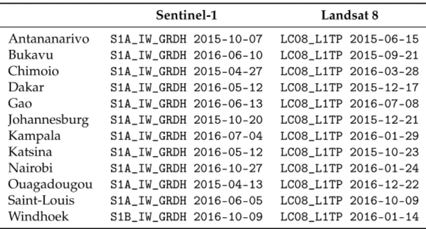
Table 2.Sentinel-1 and Landsat 8 product types and acquisition dates.

Sentinel-1 Landsat 8 Antananarivo S1A_IW_GRDH 2015-10-07 LC08_L1TP 2015-06-15 Bukavu S1A_IW_GRDH 2016-06-10 LC08_L1TP 2015-09-21 Chimoio S1A_IW_GRDH 2015-04-27 LC08_L1TP 2016-03-28 Dakar S1A_IW_GRDH 2016-05-12 LC08_L1TP 2015-12-17 Gao S1A_IW_GRDH 2016-06-13 LC08_L1TP 2016-07-08 Johannesburg S1A_IW_GRDH 2015-10-20 LC08_L1TP 2015-12-21 Kampala S1A_IW_GRDH 2016-07-04 LC08_L1TP 2016-01-29 Katsina S1A_IW_GRDH 2016-05-12 LC08_L1TP 2015-10-23 Nairobi S1A_IW_GRDH 2016-10-27 LC08_L1TP 2016-01-24 Ouagadougou S1A_IW_GRDH 2015-04-13 LC08_L1TP 2016-12-22 Saint-Louis S1A_IW_GRDH 2016-06-05 LC08_L1TP 2016-10-09 Windhoek S1B_IW_GRDH 2016-10-09 LC08_L1TP 2016-01-14

Sentinel-1 and Landsat 8 product types and acquisition dates are presented inTable 2. Landsat 8 imagery was acquired through the Earth Explorer portal of the U.S. Geological Survey (USGS) with the landsatxploresoftware [37], using cloud cover as the main criterion. Additionally, monthly NDVI values from the MODIS-based MOD13C2 dataset [38] were used to favor the most vegetated periods, which are different depending on the case study. Scenes were acquired as Level-1 data products, thus radiometrically calibrated and orthorectified. Calibrated digital numbers were converted to surface reflectance values using the Landsat Surface Reflectance Code (LaSRC) [39] made available by the USGS. Cloudy pixels were masked using the Function of Mask (FMASK) algorithm [40,41].

Sentinel-1A images were acquired through the Copernicus Open Access Hub using the sentinelsatsoftware [42]. Scenes belonging to the dry season were favored based on the monthly NDVI values provided by the MODIS-based MOD13C2 dataset. Additionally, the CPC Global Unified Precipitation dataset [43], provided by the NOAA Climate Prediction Center, was used to require at least two days without any precipitation before the acquisition date. The last criterion for the final scene selection was the temporal proximity to the selected Landsat 8 scene. The scenes were acquired as Ground Range Detected (GRD) Level-1 products in the Interferometric Wide (IW) swath mode, therefore multi-looked and projected to ground range using an Earth ellipsoid model. Preprocessing was performed using the Sentinel Application Platform (SNAP) [44]. Firstly, orbit state vectors were refined with precise orbit files and GRD data was calibrated to β nought. Then, thermal noise removal was performed before applying a speckle noise reduction based on a 3×3 Lee filter [45], in order to reduce the speckle noise while preserving the textural information. Finally, terrain flattening [46] and Range-Doppler terrain correction [47] were applied based on the SRTM 1-sec Digital Elevation Model (DEM).

2.3. Feature Extraction

Grey Level Co-Occurence Matrix (GLCM) textures were computed with an interpixel distance of 1 and 32 levels of quantization using Orfeo Toolbox [48], after a 2% histogram cutting on the source SAR data. GLCMs were constructed for the direction angles 0, 45, 90, and 135 degrees ; but only the average value was considered. The GLCMs were computed independently for each polarization (VV and VH) and multiple window sizes (5×5, 7×7, 9×9, and 11×11). A set of 18 textures was extracted: energy, entropy, correlation, inertia, cluster shade, cluster prominence, haralick correlation, mean, variance, dissimilarity, sum average, sum variance, sum entropy, difference of entropies, difference of variances, and two information measures of correlation (IC1 and IC2). This resulted in the extraction of 72 texture features for each polarization, that is, 144 in total.

Several GLCMs texture features can be highly correlated, such as energy and entropy, or inertia and the inverse different moment. In order to reduce the dimensionality of the dataset, a Principal Component Analysis (PCA) was performed on each combination of polarization and window size. Only the first six components of each PCA — which consistently explained more than 95% of the variance, were retained. This reduced the number of features from 144 to 48.

SAR features were reprojected to Universal Transverse Mercator (UTM) coordinate system only after the computation of GLCM textures in order to minimize the destruction of textural information. All Landsat 8 bands — including thermal bands, were retained without further processing except of co-registration to the spatial resolution of SAR products (i.e. about 10 meters).

2.4. Classification

The binary classification task — built-up vs. non-built-up, was performed using the Random Forest (RF) classifier, which has been shown to be relatively performant in the context of multisource and multimodal data classification [49–51]. The implementation was based on Python and a set of libraries, including: NumPy [52], SciPy [52], and Rasterio [53] for raster processing, Shapely [54] and Geopandas for vector processing and Scikit-learn [55] for machine learning. The Python code that supported the present study is available on Github (https://github.com/yannforget/landsat-sentinel-fusion), and the associated datasets can be acquired through Zenodo (https://zenodo.org/record/1450932).

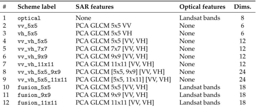
Table 3.Label, input features and number of dimensions of the 12 classification schemes.

# Scheme label SAR features Optical features Dims.

1 optical None Landsat bands 8 2 vv_5x5 PCA GLCM 5x5 VV None 6 3 vh_5x5 PCA GLCM 5x5 VH None 6 4 vv_vh_5x5 PCA GLCM 5x5 [VV, VH] None 12 5 vv_vh_7x7 PCA GLCM 7x7 [VV, VH] None 12 6 vv_vh_9x9 PCA GLCM 9x9 [VV, VH] None 12 7 vv_vh_11x11 PCA GLCM 11x11 [VV, VH] None 12 8 vv_vh_5x5_9x9 PCA GLCM [5x5, 9x9] [VV, VH] None 24 9 vv_vh_5x5_11x11 PCA GLCM [5x5, 11x11] [VV, VH] None 24 10 fusion_5x5 PCA GLCM 5x5 [VV, VH] Landsat bands 18 11 fusion_9x9 PCA GLCM 9x9 [VV, VH] Landsat bands 18 12 fusion_11x11 PCA GLCM 11x11 [VV, VH] Landsat bands 18

In order to assess the optimal combination of features in the context of a pixel-based supervised classification, 12 different classifications were performed using different input features.Table 3lists the features used for each classification scheme. The schemes #1 to #9 were single-source classifications, based either on optical or SAR data. Previous studies suggested that combining several window sizes could improve classification accuracies by including spatial information from multiple scales [56]. The schemes #2 to #9 were designed to identify the optimal window size and polarization combination to classify built-up areas using Sentinel-1. Finally, the schemes #10 to #12 included both optical and SAR data with different window sizes for the computation of the GLCMs.

In the 12 classification schemes, the RF ensemble was constructed with 50 trees and a maximum number of features per tree equal to the square root of the total number of features — as suggested by previous studies [50]. Imbalance issues in the training dataset between the built-up and the non-built-up classes were overcome by a random over-sampling of the minority class [57]. Additionally, in order to ensure the reproducibility of the results, fixed random seeds were used.

2.5. Validation

Reference polygons were digitized from very high spatial resolution imagery through Google Earth to support both the training and the validation of the classification models. Four land cover

classes were collected: built-up, bare soil, low vegetation (sparse or small vegetation), and high vegetation (dense and tall vegetation). All non-built-up samples (bare soil, low vegetation and high vegetation) were concatenated to build the binary (built-up vs. non-built-up) training and validation datasets. However, specific land cover samples were also used to assess the performance of the models in specific areas.Table 4shows the number of polygons collected for each land cover and each case study, together with the amount of resulting samples (in pixels) after rasterization.

Table 4. Number of reference pixels for each case study and land cover. Enclosed in brackets: the number of polygons before rasterization.

Built-up Bare Soil Low Vegetation High Vegetation

Antananarivo 42,596 (110) 31,769 (67) 60,423 (53) 22,338 (50) Bukavu 30,762 (54) 5,956 (20) 19,196 (21) 7,308 (22) Chimoio 29,040 (79) 17,405 (59) 11,891 (63) 11,347 (50) Dakar 123,386 (76) 14,367 (41) 60,993 (53) 29,739 (33) Gao 18,998 (74) 46,834 (45) 805 (25) 1,348 (25) Johannesburg 570,282 (260) 69,106 (91) 97,100 (112) 26,315 (37) Kampala 41,528 (89) 5,049 (34) 21,033 (44) 9,376 (22) Katsina 37,507 (95) 11,710 (55) 4,411 (31) 2,107 (28) Nairobi 60,371 (103) 15,030 (46) 18,947 (41) 12,666 (23) Ouagadougou 83,540 (62) 22,477 (24) 66,624 (15) 26,078 (7) Saint-Louis 13,154 (64) 24,162 (47) 25,701 (40) 10,388 (22) Windhoek 62,464 (60) 50,247 (79) 26,032 (48) 14,655 (28)

In order to ensure the independence of the training and validation datasets, the reference samples were randomly splitted at the polygon level — the samples inside a given polygon being characterized by a high spatial autocorrelation. Each classification is performed ten times with different random splits, then assessment metrics (F1-score, land cover accuracies) and classifier characteristics (feature importances, probabilities) were averaged for statistical and visual interpretation.

3. Results and Discussion

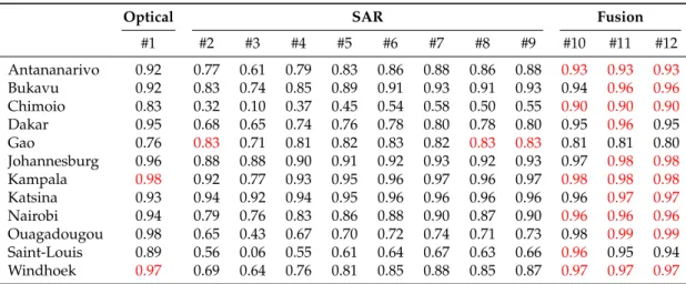
Table 5. F1-score obtained by each classification scheme in each case study (seeTable 3for the characteristics of each scheme). In red: best F1-score for a given case study.

Optical SAR Fusion

#1 #2 #3 #4 #5 #6 #7 #8 #9 #10 #11 #12 Antananarivo 0.92 0.77 0.61 0.79 0.83 0.86 0.88 0.86 0.88 0.93 0.93 0.93 Bukavu 0.92 0.83 0.74 0.85 0.89 0.91 0.93 0.91 0.93 0.94 0.96 0.96 Chimoio 0.83 0.32 0.10 0.37 0.45 0.54 0.58 0.50 0.55 0.90 0.90 0.90 Dakar 0.95 0.68 0.65 0.74 0.76 0.78 0.80 0.78 0.80 0.95 0.96 0.95 Gao 0.76 0.83 0.71 0.81 0.82 0.83 0.82 0.83 0.83 0.81 0.81 0.80 Johannesburg 0.96 0.88 0.88 0.90 0.91 0.92 0.93 0.92 0.93 0.97 0.98 0.98 Kampala 0.98 0.92 0.77 0.93 0.95 0.96 0.97 0.96 0.97 0.98 0.98 0.98 Katsina 0.93 0.94 0.92 0.94 0.95 0.96 0.96 0.96 0.96 0.96 0.97 0.97 Nairobi 0.94 0.79 0.76 0.83 0.86 0.88 0.90 0.87 0.90 0.96 0.96 0.96 Ouagadougou 0.98 0.65 0.43 0.67 0.70 0.72 0.74 0.71 0.73 0.98 0.99 0.99 Saint-Louis 0.89 0.56 0.06 0.55 0.61 0.64 0.67 0.63 0.66 0.96 0.95 0.94 Windhoek 0.97 0.69 0.64 0.76 0.81 0.85 0.88 0.85 0.87 0.97 0.97 0.97

Table 5presents the F1-score obtained with each classification scheme in each case study. In 10 case studies out of 12, optical-based schemes reached a higher F1-score than SAR-based schemes. The two case studies where SAR-based schemes appears more accurate are Gao (+7.6 points) and Katsina (+3.4 points): two small urban areas located in an arid climate characterized by a domination of bare land in the landscape. However, the trend is not confirmed by the low scores obtained by SAR-based schemes

in cities such as Ouagadougou and Saint-Louis, which present similar characteristics. These results suggest that optical-based schemes are superior to SAR-based schemes in the context of pixel-based classifications from a single sensor. This can be explained by the speckle noise inherent to SAR data and by the loss of spatial resolution that occured during the computation of the GLCM textures. However, in 11 case studies out of 12, the multi-sensor classification schemes reached the highest F1-scores — the only exception being Gao, where the SAR-based scheme performed better. In most of the case studies, complementing optical data with SAR features improved the classification performances, sometimes dramatically (+6.7 points in Chimoio, +6.6 in Saint-Louis, +5.8 in Gao, +4 in Bukavu and Katsina). This suggests that combining optical and SAR-based GLCM textures in the context of a pixel-based classification can be a reliable and robust strategy.

0.3 0.4 0.5 0.6 0.7 0.8 0.9 1.0 F1-score Optical SAR VV 5x5 SAR VH 5x5 SAR VV VH 5x5 SAR VV VH 7x7 SAR VV VH 9x9 SAR VV VH 11x11 SAR VV VH 5x5 9x9 SAR VV VH 5x5 11x11 Fusion 5x5 Fusion 9x9 Fusion 11x11

Figure 1.Box plot of the F1-score obtained with each classification scheme for each case study.

The performance of each classification scheme is summarised inFigure 1, which confirms the previously observed trends. The difference between the various SAR-based classification schemes is also highlighted. Classifications based on the VV polarization reached higher scores compared to the ones based on the VH polarization. However, combining texture features derived from both polarizations appears to increase the reliability of the classification models, leading to higher scores and a lower standard deviation. Likewise, the window size used for the computation of the GLCM did influence the classification scores. In our case studies, larger window sizes led to higher scores and reduced the variability across the case studies. We previously stated the hypothesis that combining several window sizes could increase the classification performance by including spatial information from multiple scales. The results obtained tend to refute this hypothesis, as the schemes combining textures from two window sizes did not perform better. Generally, the fusion schemes consistently obtained the highest scores. However, contrary to the trend observed in single-sensor SAR-based schemes, combining optical data with larger window sizes textures does not seem to increase the classification performance. Fusion schemes that include textures computed with smaller window sizes (5×5 and 9×9) benefited from slightly less variability across the case studies.

0% 25% 50% 75% 100% Antananarivo Bukavu Chimoio Dakar Gao Johannesburg Kampala Katsina Nairobi Ouagadougou Saint-Louis Windhoek VV VH Multispectral Thermal

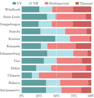
Figure 2.Grouped Random Forest feature importances for the fusion scheme in each case study. VV and VH groups correspond to the SAR features derived from a given polarization. Multispectral and thermal groups correspond to the Landsat 8 bands.

In classifiers based on a forest of decision trees such as RF, the relative contribution of each feature can be evaluated through the feature importance measure. The value ranges from 0.0 to 1.0, where 0.0 would indicate a feature that does not contribute to the classification, and 1.0 a feature that alone classifies all samples. Figure 2shows the repartition of the importance measure across the input features used in the fusion classification scheme, grouped by data source: VV or VH polarization for SAR data, and multispectral or thermal for optical data. Generally, texture features derived from the VV polarization and multispectral bands from Landsat 8 were the features contributing the most to the construction of the decision trees. Considering the lower scores obtained in single-sensor classification schemes with SAR data, lower importances for SAR features could be expected. However, the grouped importance of SAR features was superior to the importance of optical features in 5 case studies, and exceeded 40% of the contribution in 10 case studies. Furthermore, the relative importance of optical and SAR features did not appear correlated with their respective scores in the context of a single-sensor classification. For instance, in Antananarivo and Nairobi, the best SAR-based classification scheme reached a F1-score lower than the optical-based scheme by, respectively, 4.2 and 3.9 points. However, in the context of the fusion scheme, the contribution of SAR features was superior to the contribution of optical features. This suggests that the combination of both optical and SAR features adds information to the classifier that cannot be modeled in the context of a single-sensor classification.

0.70

0.75

0.80

0.85

0.90

0.95

1.00

Accuracy

Fusion 11x11

Fusion 9x9

Fusion 5x5

SAR VV VH 5x5 11x11

SAR VV VH 5x5 9x9

SAR VV VH 11x11

SAR VV VH 9x9

SAR VV VH 7x7

SAR VV VH 5x5

SAR VH 5x5

SAR VV 5x5

Optical

Bare soil

Low vegetation

High vegetation

Figure 3.Classification accuracy in specific land covers for each scheme.

As previously stated, combining SAR-based textural information and optical imagery is expected to improve the classification performance in bare lands.Figure 3shows the mean accuracy of each classification scheme in three non-built-up land covers: bare soil, low vegetation and high vegetation. As expected, the performance of the classification model in bare soil areas was superior in SAR-based schemes than in optical-based schemes. On the contrary, SAR-based classification schemes, especially the ones based on the VH polarization, suffered from low accuracies in densely vegetated areas. Finally, fusion schemes based on both SAR and optical data benefited from the complementarity between both sensors and present high accuracies in the three land covers.

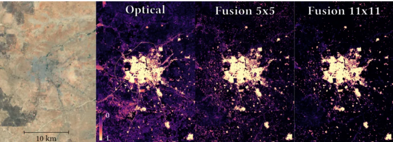
Figure 4. Random Forest class probabilities in Katsina, Nigeria. a) Aerial view of the case study;

b) optical scheme probabilities; c) fusion_5x5 scheme probabilities; d) fusion_11x11 scheme probabilities. Satellite imagery courtesy of Google.

Figure 4shows the probabilistic output of three different classifiers: one based only on optical data, and two based on both optical and SAR data with different GLCM window sizes. Visually, the fusion classifiers appears to better distinguish between the built-up areas and the surrounding bare lands. This leads to lower rates of misclassification after thresholding of the probabilities, as previously shown by the assessment metrics. A side effect of the data fusion is the disappearance of the road

network from the built-up class. Indeed, the classifier highly relies on the textural information from the SAR features to discriminate between built-up and bare land, and roads are therefore excluded from the built-up class.

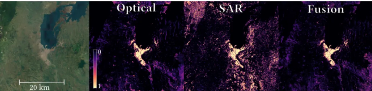
Figure 5.Random Forest class probabilities in Bukavu, D. R. Congo. a) Aerial view of the case study; b) opticalscheme probabilities; c) sar_vv_vh_5x5_11x11 scheme probabilities; d) fusion_11x11 scheme probabilities. Satellite imagery courtesy of Google.

There is some cases where data fusion is less beneficial.Figure 5shows the probabilistic output of the optical, SAR, and fusion schemes in Bukavu. This case study, located in a mountainous area, presents two major obstacles for SAR data: dense vegetation in the north-west and steep slopes in the south-east. Mapping the probabilistic output of the SAR-based classifier reveals the confusion occurring in these areas. As a result, the probabilistic output of the fusion-based classifier appears nearly as a copy of the optical-based one.

4. Conclusion

With the increasing availability of free imagery from multiple sensors such as Sentinel-1 and Landsat 8, data fusion is one of the main challenge in remote sensing. The objective of this paper was to assess the combined use of both Landsat 8 and Sentinel-1 imagery with a fusion scheme that relies on a simple pixel-based classifier. The main expectation was a better discrimination between built-up and bare soil areas in the context of urban mapping in Sub-Saharan Africa. The presented results suggest that the complementarity between medium resolution optical and SAR sensors can be exploited in the context of a supervised pixel-based classification. However, to make the pixel-based approach effective, textural information must be extracted from SAR backscattering in order to reduce the speckle noise and to provide contextual information at the pixel level.

Classification schemes including both optical and SAR features reached the highest scores in 11 case studies out of 12. Single-sensor classifiers making use of GLCM textures derived from the VV polarization outperformed the ones based on the VH polarization. Nevertheless, combining both polarizations consistently increased the classification performance. Likewise, large GLCM window sizes (9×9 or 11×11) provided a slight improvement of the classification performance both in the context of single-sensor classification and in fusion schemes. However, contrary to an hypothesis that we formulated, combining textures derived from multiple GLCM window sizes — in order to include spatial information from multiple scales at the pixel level, did not lead to a better classification performance. The visual interpretation of the results obtained suggests that small GLCM window sizes favor the detection of isolated settlements and buildings, whereas larger window sizes lead to a better differentiation between built-up areas and bare lands. In the context of this study, the RF classifier was not able to take advantage of both.

The assessment of the classifiers performances in specific land covers confirmed the high level of complementarity between the two sensors. Single-sensor SAR-based classifications presented high accuracies in bare soil areas, but suffered from a confusion between dense vegetation and buildings. On the contrary, optical-based classifiers showed a high ability to discriminate between vegetation and built-up, but a low differentiation between bare soil and built-up — especially in the most arid

landscapes such as in Gao or Katsina. This complementarity was correctly modeled by the RF classifier and, as a result, the fusion schemes presented high accuracies in both bare lands and vegetated areas. Nevertheless, the fusion was less beneficial in case studies characterized by the presence of dense vegetation and steep slopes — for instance in a mountainous and subtropical urban areas such as Bukavu. However, in this case, the RF classifier was able to learn from the training dataset that SAR data were not reliable. This suggests that including features derived from a DEM — for instance slope and aspect, could improve the model ability to quantify the reliability of SAR data at the pixel level. Such a strategy could also take place at the decision level. Further work is also required to assess the reliability of the presented approach in the context of similar sensors such as Sentinel-2, ERS-1 and ERS-2.

Author Contributions:Conceptualization, Yann Forget, Michal Shimoni, Marius Gilbert and Catherine Linard; Data curation, Yann Forget; Formal analysis, Yann Forget and Michal Shimoni; Funding acquisition, Michal Shimoni, Marius Gilbert and Catherine Linard; Investigation, Yann Forget; Methodology, Yann Forget and Michal Shimoni; Project administration, Michal Shimoni, Marius Gilbert and Catherine Linard; Resources, Marius Gilbert and Catherine Linard; Software, Yann Forget; Supervision, Michal Shimoni, Marius Gilbert and Catherine Linard; Validation, Yann Forget, Michal Shimoni and Catherine Linard; Visualization, Yann Forget; Writing – original draft, Yann Forget; Writing – review & editing, Yann Forget, Michal Shimoni, Marius Gilbert and Catherine Linard.

Funding: This research was funded by the Belgian Science Policy Office and is part of the research project SR/00/304 MAUPP (Modelling and Forecasting African Urban Population Patterns for Vulnerability and Health Assessments).

Conflicts of Interest:The authors declare no conflict of interest.

1. Grimm, N.B.; Faeth, S.H.; Golubiewski, N.E.; Redman, C.L.; Wu, J.; Bai, X.; Briggs, J.M. Global Change and the Ecology of Cities. Science 2008, 319, 756–760. doi:10.1126/science.1150195.

2. Dye, C. Health and Urban Living. Science 2008, 319, 766–769. doi:10.1126/science.1150198.

3. UN-Habitat. Sustainable Urban Development in Africa. Technical report, UN-Habitat, Nairobi, Kenya, 2015.

4. Linard, C.; Tatem, A.J.; Gilbert, M. Modelling Spatial Patterns of Urban Growth in Africa. Applied Geography

2013, 44, 23–32. doi:10.1016/j.apgeog.2013.07.009.

5. Gamba, P.; Herold, M. Global Mapping of Human Settlement: Experiences, Datasets, and Prospects; Taylor & Francis series in remote sensing applications, CRC Press: Boca Raton, 2009.

6. Wentz, E.; Anderson, S.; Fragkias, M.; Netzband, M.; Mesev, V.; Myint, S.; Quattrochi, D.; Rahman, A.; Seto, K. Supporting Global Environmental Change Research: A Review of Trends and Knowledge Gaps in Urban Remote Sensing. Remote Sensing 2014, 6, 3879–3905. doi:10.3390/rs6053879.

7. Forster, B.C. Coefficient of Variation as a Measure of Urban Spatial Attributes, Using SPOT HRV and Landsat TM Data. International Journal of Remote Sensing 1993, 14, 2403–2409. doi:10.1080/01431169308954044.

8. Small, C. Multiresolution Analysis of Urban Reflectance. IEEE/ISPRS Joint Workshop on Remote Sensing and Data Fusion over Urban Areas; IEEE: Rome, Italy, 2001; pp. 15–19. doi:10.1109/DFUA.2001.985717. 9. Small, C. A Global Analysis of Urban Reflectance. International Journal of Remote Sensing 2005, 26, 661–681. 10. Potere, D.; Schneider, A.; Angel, S.; Civco, D. Mapping Urban Areas on a Global Scale: Which of the Eight Maps Now Available Is More Accurate? International Journal of Remote Sensing 2009, 30, 6531–6558. doi:10.1080/01431160903121134.

11. Kottek, M.; Grieser, J.; Beck, C.; Rudolf, B.; Rubel, F. World Map of the Köppen-Geiger Climate Classification Updated. Meteorologische Zeitschrift 2006, 15, 259–263. doi:10.1127/0941-2948/2006/0130.

12. Rubel, F.; Brugger, K.; Haslinger, K.; Auer, I. The Climate of the European Alps: Shift of Very High Resolution Köppen-Geiger Climate Zones 1800–2100. Meteorologische Zeitschrift 2017, 26, 115–125. doi:10.1127/metz/2016/0816.

13. Qian, J.; Zhou, Q.; Hou, Q. Comparison of Pixel-Based and Object-Oriented Classification Methods for Extracting Built-up Areas in Arid Zone. ISPRS Workshop on Updating Geo-Spatial Databases with Imagery & The 5th ISPRS Workshop on DMGISs; , 2007; pp. 163–171.

14. Rasul, A.; Balzter, H.; Ibrahim, G.; Hameed, H.; Wheeler, J.; Adamu, B.; Ibrahim, S.; Najmaddin, P. Applying Built-Up and Bare-Soil Indices from Landsat 8 to Cities in Dry Climates. Land 2018, 7, 81. doi:10.3390/land7030081.

15. Zhang, C.; Chen, Y.; Lu, D. Mapping the Land-Cover Distribution in Arid and Semiarid Urban Landscapes with Landsat Thematic Mapper Imagery. International Journal of Remote Sensing 2015, 36, 4483–4500. doi:10.1080/01431161.2015.1084552.

16. Li, H.; Wang, C.; Zhong, C.; Su, A.; Xiong, C.; Wang, J.; Liu, J. Mapping Urban Bare Land Automatically from Landsat Imagery with a Simple Index. Remote Sensing 2017, 9, 249. doi:10.3390/rs9030249.

17. Weng, Q. Global Urban Monitoring and Assessment through Earth Observation; Crc Press, 2014.

18. Soergel, U. Radar Remote Sensing of Urban Areas; Number v. 15 in Remote sensing and digital image processing, Springer: Dordrecht ; New York, 2010.

19. Waske, B.; van der Linden, S. Classifying Multilevel Imagery From SAR and Optical Sensors by Decision Fusion. IEEE Transactions on Geoscience and Remote Sensing 2008, 46, 1457–1466. doi:10.1109/TGRS.2008.916089.

20. Zhang, H.; Zhang, Y.; Lin, H. A Comparison Study of Impervious Surfaces Estimation Using Optical and SAR Remote Sensing Images. International Journal of Applied Earth Observation and Geoinformation 2012, 18, 148–156. doi:10.1016/j.jag.2011.12.015.

21. Joshi, N.; Baumann, M.; Ehammer, A.; Fensholt, R.; Grogan, K.; Hostert, P.; Jepsen, M.; Kuemmerle, T.; Meyfroidt, P.; Mitchard, E.; Reiche, J.; Ryan, C.; Waske, B. A Review of the Application of Optical and Radar Remote Sensing Data Fusion to Land Use Mapping and Monitoring. Remote Sensing 2016, 8, 70. doi:10.3390/rs8010070.

22. Tupin, F. Fusion of Optical and SAR Images. In Radar Remote Sensing of Urban Areas; Soergel, U., Ed.; Number 15 in Remote sensing and digital image processing, Springer: Dordrecht ; New York, 2010; pp. 133–159.

23. Griffiths, P.; Hostert, P.; Gruebner, O.; van der Linden, S. Mapping Megacity Growth with Multi-Sensor Data. Remote Sensing of Environment 2010, 114, 426–439. doi:10.1016/j.rse.2009.09.012.

24. Zhu, Z.; Woodcock, C.E.; Rogan, J.; Kellndorfer, J. Assessment of Spectral, Polarimetric, Temporal, and Spatial Dimensions for Urban and Peri-Urban Land Cover Classification Using Landsat and SAR Data. Remote Sensing of Environment 2012, 117, 72–82. doi:10.1016/j.rse.2011.07.020.

25. Zhang, Y.; Zhang, H.; Lin, H. Improving the Impervious Surface Estimation with Combined Use of Optical and SAR Remote Sensing Images. Remote Sensing of Environment 2014, 141, 155–167. doi:10.1016/j.rse.2013.10.028.

26. Braun, A.; Hochschild, V. Combined Use of SAR and Optical Data for Environmental Assessments around Refugee Camps in Semiarid Landscapes. ISPRS - International Archives of the Photogrammetry, Remote Sensing and Spatial Information Sciences 2015, XL-7/W3, 777–782. doi:10.5194/isprsarchives-XL-7-W3-777-2015. 27. Clerici, N.; Valbuena Calderón, C.A.; Posada, J.M. Fusion of Sentinel-1A and Sentinel-2A Data for Land

Cover Mapping: A Case Study in the Lower Magdalena Region, Colombia. Journal of Maps 2017, 13, 718–726. doi:10.1080/17445647.2017.1372316.

28. Benediktsson, J.A.; Kanellopoulos, I. Classification of Multisource and Hyperspectral Data Based on Decision Fusion. Geoscience and Remote Sensing, IEEE Transactions on 1999, 37, 1367–1377.

29. Fauvel, M.; Chanussot, J.; Benediktsson, J. Decision Fusion for the Classification of Urban Remote Sensing Images. IEEE Transactions on Geoscience and Remote Sensing 2006, 44, 2828–2838. doi:10.1109/TGRS.2006.876708.

30. Shao, Z.; Fu, H.; Fu, P.; Yin, L. Mapping Urban Impervious Surface by Fusing Optical and SAR Data at the Decision Level. Remote Sensing 2016, 8, 945. doi:10.3390/rs8110945.

31. Gamba, P. Image and Data Fusion in Remote Sensing of Urban Areas: Status Issues and Research Trends. International Journal of Image and Data Fusion 2014, 5, 2–12. doi:10.1080/19479832.2013.848477.

32. Haralick, R.M.; Shanmugam, K.; Dinstein, I. Textural Features for Image Classification. IEEE Transactions on Systems, Man, and Cybernetics 1973, SMC-3, 610–621. doi:10.1109/TSMC.1973.4309314.

33. Gotlieb, C.C.; Kreyszig, H.E. Texture Descriptors Based on Co-Occurrence Matrices. Computer Vision, Graphics, and Image Processing 1990, 51, 70–86. doi:10.1016/S0734-189X(05)80063-5.

34. NASA JPL. NASA Shuttle Radar Topography Mission Global 1 Arc Second. NASA EOSDIS Land Processes DAAC 2013. doi:10.5067/MEaSUREs/SRTM/SRTMGL1.003.

35. Linard, C.; Gilbert, M.; Snow, R.W.; Noor, A.M.; Tatem, A.J. Population Distribution, Settlement Patterns and Accessibility across Africa in 2010. PLoS ONE 2012, 7. doi:10.1371/journal.pone.0031743.

36. Worldpop. Africa 1km Population. http://www.worldpop.org.uk/data/summary/?doi=10.5258/ SOTON/WP00004, 2016. Accessed: 2018-10-07, doi:10.5258/SOTON/WP00004.

37. Forget, Y. Landsatxplore. https://github.com/yannforget/landsatxplore, 2018. Accessed: 2018-10-07, doi:10.5281/zenodo.1291423.

38. Didan, K. MOD13C2 MODIS/Terra Vegetation Indices Monthly L3 Global 0.05Deg CMG V006. https: //lpdaac.usgs.gov/node/843, 2015. Accessed: 2018-10-07, doi:10.5067/MODIS/MOD13C2.006.

39. Vermote, E.; Justice, C.; Claverie, M.; Franch, B. Preliminary Analysis of the Performance of the Landsat 8/OLI Land Surface Reflectance Product. Remote Sensing of Environment 2016, 185, 46–56. doi:10.1016/j.rse.2016.04.008.

40. Zhu, Z.; Woodcock, C.E. Object-Based Cloud and Cloud Shadow Detection in Landsat Imagery. Remote Sensing of Environment 2012, 118, 83–94. doi:10.1016/j.rse.2011.10.028.

41. Zhu, Z.; Wang, S.; Woodcock, C.E. Improvement and Expansion of the Fmask Algorithm: Cloud, Cloud Shadow, and Snow Detection for Landsats 4–7, 8, and Sentinel 2 Images. Remote Sensing of Environment

2015, 159, 269–277. doi:10.1016/j.rse.2014.12.014.

42. Clauss, K.; Valgur, M.; Marcel, W.; Sølvsteen, J.; Delucchi, L.; Unnic.; Kinyanjui, L.K.; Schlump.; Martinber.; Baier, G.; Keller, G.; Castro, C. Sentinelsat. https://github.com/sentinelsat/sentinelsat, 2018. Accessed: 2018-10-07, doi:10.5281/zenodo.595961.

43. Chen, M.; Shi, W.; Xie, P.; Silva, V.B.S.; Kousky, V.E.; Wayne Higgins, R.; Janowiak, J.E. Assessing Objective Techniques for Gauge-Based Analyses of Global Daily Precipitation. Journal of Geophysical Research 2008, 113. doi:10.1029/2007JD009132.

44. ESA. Sentinel Application Platform (SNAP).http://step.esa.int, 2018. Accessed: 2018-10-07.

45. Lee, J.S. Speckle Analysis and Smoothing of Synthetic Aperture Radar Images. Computer Graphics and Image Processing 1981, 17, 24–32. doi:10.1016/S0146-664X(81)80005-6.

46. Small, D. Flattening Gamma: Radiometric Terrain Correction for SAR Imagery. IEEE Transactions on Geoscience and Remote Sensing 2011, 49, 3081–3093. doi:10.1109/TGRS.2011.2120616.

47. Small, D.; Shubert, A. Guide to ASAR Geocoding. RSL-ASAR-GC-AD 2008.

48. Grizonnet, M.; Michel, J.; Poughon, V.; Inglada, J.; Savinaud, M.; Cresson, R. Orfeo ToolBox: Open Source Processing of Remote Sensing Images. Open Geospatial Data, Software and Standards 2017, 2. doi:10.1186/s40965-017-0031-6.

49. Pal, M. Random Forest Classifier for Remote Sensing Classification. International Journal of Remote Sensing

2005, 26, 217–222. doi:10.1080/01431160412331269698.

50. Gislason, P.O.; Benediktsson, J.A.; Sveinsson, J.R. Random Forests for Land Cover Classification. Pattern Recognition Letters 2006, 27, 294–300. doi:10.1016/j.patrec.2005.08.011.

51. Belgiu, M.; Dr˘agu¸t, L. Random Forest in Remote Sensing: A Review of Applications and Future Directions. ISPRS Journal of Photogrammetry and Remote Sensing 2016, 114, 24–31. doi:10.1016/j.isprsjprs.2016.01.011. 52. Oliphant, T.E. Python for Scientific Computing. Computing in Science & Engineering 2007, 9, 10–20.

doi:10.1109/MCSE.2007.58.

53. Gillies, S. Rasterio: Geospatial Raster I/O for Python Programmers.https://github.com/mapbox/rasterio, 2013. Accessed: 2018-10-07.

54. Gillies, S. Shapely: Manipulation and Analysis of Geometric Objects. http://toblerity.github.com/ shapely/, 2007. Accessed: 2018-10-07.

55. Pedregosa, F.; Varoquaux, G.; Gramfort, A.; Michel, V.; Thirion, B.; Grisel, O.; Blondel, M.; Prettenhofer, P.; Weiss, R.; Dubourg, V. Scikit-Learn: Machine Learning in Python. Journal of Machine Learning Research 2011, 12, 2825–2830.

56. Puissant, A.; Hirsch, J.; Weber, C. The Utility of Texture Analysis to Improve Per-pixel Classification for High to Very High Spatial Resolution Imagery. International Journal of Remote Sensing 2005, 26, 733–745. doi:10.1080/01431160512331316838.

57. Lemaître, G.; Nogueira, F.; Aridas, C.K. Imbalanced-Learn: A Python Toolbox to Tackle the Curse of Imbalanced Datasets in Machine Learning. Journal of Machine Learning Research 2017, 18, 1–5.