Simple and yet novel approach in flood assessment to overcome data scarcity : high quality DEM and rainfall proxies

(1)

HAL Id: tel-02492281

https://tel.archives-ouvertes.fr/tel-02492281

Submitted on 26 Feb 2020

HAL is a multi-disciplinary open access archive for the deposit and dissemination of sci-entific research documents, whether they are pub-lished or not. The documents may come from teaching and research institutions in France or

L’archive ouverte pluridisciplinaire HAL, est destinée au dépôt et à la diffusion de documents scientifiques de niveau recherche, publiés ou non, émanant des établissements d’enseignement et de recherche français ou étrangers, des laboratoires

Simple and yet novel approach in flood assessment to

overcome data scarcity : high quality DEM and rainfall

proxies

Dong Eon Kim

To cite this version:

Dong Eon Kim. Simple and yet novel approach in flood assessment to overcome data scarcity : high quality DEM and rainfall proxies. Risques. COMUE Université Côte d’Azur (2015 - 2019), 2019. English. �NNT : 2019AZUR4029�. �tel-02492281�

(2)

Approche simple et novatrice pour

l’évaluation des inondations dans un context

e

pauvre en données

:

Solutions alternatives aux MNT haute résolution et aux

données locales de précicipitation

Dong Eon KIM

Polytech Lab

Présentée en vue de l’obtention du grade de docteur en discipline d’Université Côte d’Azur

Dirigée par : Philippe GOURBESVILLE Co-encadrée par : Shie-Yui LIONG Soutenue le : 10 Juin 2019

Devant le jury, composé de :

Reinhard HINKELMANN, Pr., TU Berlin, Allemagne

Manuel GOMEZ VALENTIN, Pr., Université Politecnica de Catalunya, Espagne

Shie-Yui LIONG, Pr., Université Nationale de Singapour, Singapour

Philippe AUDRA, Pr., Université Nice Sophia Antipolis

Philippe GOURBESVILLE, Pr., Université Nice Sophia Antipolis Ludovic ANDRES, Métropole Nice Côte d'Azur

(3)

ACKNOWLEDGEMENT

Pursuing a PhD program is both enjoyable and painful experience in my life journey. At the beginning of my study, I was very confident about what to do and what will have to be done. However, it was not as straightforward as I initially thought. I met obstacles even on the first step and had difficulty to solve the problems. When the issues were settled after various twists and turns, I regained the confidence that I could settle anything in the future. However, these up and down cycles repeated until the end of this PhD study. The experience gained from this PhD program surely prepare me to face challenges in both my future carrier and personal life.

Whenever I was steeped in anxiety, there were always people around me who comforted and strengthened me. I would like to express my deepest appreciation to all these people. First and foremost, I would like to express my sincere thanks to my supervisors, Professor Philippe Gourbesville and Professor Shie-Yui Liong, for their contributions in providing suggestions, feedbacks and many other countless supports. Without their support, I would never have completed my PhD program.

Special thanks are also extended to my colleagues since I started my PhD: Dr. Jiandong Liu, Dr. Srivatsan Vijayaraghavan, Dr. Yabin Sun, Dr. Dadiyorto Wendi, Dr. Chi Dung Doan, Dr. Qiang Ma and Dr. Lian Guey Ler. They, aside from being my good friends, helped me in providing the necessary data and ideas leading to the present quality of my study. I had excellent time with them; I surely treasure our friendship.

I also wish to extend my appreciation to all those organizations and persons who made their invaluable data available to me: (1) Dr. Ludovic Andres of Nice Côte d'Azur Metropolis for providing the extremely high resolution DEM of Nice; (2) German Aerospace Center (DLR) for TanDEM-X; (3) National Aeronautics and Space Administration (NASA) for SRTM; and (4) European Space Agency (ESA) for Sentinel-2

Last, but not least, I am greatly indebted to my wife, Soo Yeon, and my kids, Do Yeon and Min Geon. They are absolutely the source of my happiness. Their love and support have encouraged me to fully focus on and complete this PhD program with excellent results. Thank you.

(4)

iii

ABSTRACT

Simple-and-yet-novel approach in flood assessment to overcome data scarcity: High quality DEM and rainfall proxies

Many urban cities in Southeast Asia witness severe flooding associated to increasing rainfall intensity and rapid urbanization often due to poor urban planning. Two important inputs required in flood hazard assessment are: (1) high accuracy Digital Elevation Model (DEM), and (2) long rainfall record. High accuracy DEM is both expensive and time consuming to acquire. Long rainfall records for areas of interest are often not available or not sufficiently long to determine the probable extremes. This thesis presents a notably cost-effective and efficient approach to estimate high-resolution and accuracy DEM, and suggests proxies for long rainfall data.

DEM data from a publicly accessible satellite, Shuttle Radar Topography Mission (SRTM), and Sentinel 2 multispectral imagery are selected and used to train the Artificial Neural Network (ANN) to improve the quality of the DEM. In the training of ANN, high quality observed DEM is the key leading to a well-trained ANN. The trained ANN will then be ready to efficiently and effectively generate high quality DEM, at low cost, for places where DEM data is not available.

The performance of the DEM improvement scheme is evaluated in places of various landuse types (e.g. dense urban areas, forested areas), and in different countries (Nice, France; Singapore; Jakarta, Indonesia) through various criteria, e.g. whenever possible visual clarity, scatter plots, Root Mean Square Error (RMSE) and drainage networks. The DEM resulting from the latest version of improved SRTM (iSRTM_v2 DEM) performs (1) significantly better than the original SRTM DEM, a 34 % to 57 % RMSE reduction; (2) the visual clarity is so much better; and (3) much closer drainage network with the actual. The much improved DEM allows flood modelling to proceed with high confidence. Rainfall data resulting from a high spatial resolution Regional Climate Model (RCM), Weather Research and Forecasting driven by ERA-Interim (WRF/ERAI) dataset, is extracted, analyzed, and compared with high quality observed rainfall data of Singapore with regard to accuracy. The comparisons are performed, among others, on their Intensity-Duration-Frequency (IDF) curves, the essential design curves for flood risk assessment; they matched quite well. The rainfall data (from the RCM) are then used as proxies for Greater Jakarta (Indonesia), where no rainfall data were available, to derive the IDF curves required for the flood analysis.

MIKE 21 Flow Model Flexible Mesh (MIKE 21 FM) is applied to Greater Jakarta, with input data from the above mentioned much improved DEM and precipitation proxy data, for flood simulations

(5)

of 2 return periods (50- and 100-years). Qualitative agreement of model results and observation of the 2013 Jakarta flood were obtained. This demonstrates the applications of the approaches/methodologies, proposed in this thesis, on catchments where most essential data for flood risk assessment (high resolution and high accuracy DEM and long and high accuracy rainfall data) are not available.

This thesis should be of interest to readers of the areas of remote sensing, artificial intelligence and flood management, possibly also for the policy makers in proposing relevant flood mitigation measures under climate change with increasing devastating flood damages and casualties.

(6)

v

RESUME

De nombreuses villes d’Asie du Sud-Est subissent de graves inondations liées d’une part à l’intensité croissante des précipitations et part d’autre à une urbanisation rapide souvent due à une planification urbaine non maitrisée. L'évaluation quantitative des risques d'inondation nécessite deux éléments essentiels: (1) un modèle numérique de terrain (MNT) haute définition, et (2) une chronologie de précipitations la plus longue possible. Un MNT haute définition est à la fois coûteux et long à acquérir. Les chronologies de précipitations longues sont fréquemment indisponibles dans de nombreux sites et ne présentent pas toujours une durée suffisante pour une définition pertinente des valeurs extrêmes. Cette thèse présente une approche opérationnelle pour générer des MNT haute définition et suggère une stratégie pour définir des pluies extrêmes en dehors de chronologies de précipitations longues.

Des données pour la production des MNT issues de capteurs satellitaires - mission SRTM (Shuttle Radar Topography Mission) et images multi spectrales Sentinel 2 - ont été utilisées et mises en œuvre. Un réseau de neurones artificiels (ANN) est utilisé afin d'améliorer la qualité du MNT. Dans la phase d’apprentissage du réseau de neurones, la qualité des MNE utilisés comme référence est essentielle et conditionne la performance de l’outil dans son application ultérieure. A la suite de cet apprentissage, le réseau de neurones peut être mis en œuvre pour générer, à faible coût, des MNT haute résolution dans des secteurs où les données sont partiellement indisponibles.

Les performances de la méthode d’amélioration du MNT sont évaluées dans des différents secteurs caractérisés par des occupations du sol variées (secteur urbain dense, secteurs boisés par exemple) et dans différents pays (Nice, France; Singapour; Jakarta, Indonésie). La qualité des résultats est analysées avec différents indicateurs tels que les diagrammes de dispersion, la clarté visuelle, l’erreur quadratique moyenne (RMSE) et l’adéquation avec les réseaux de drainage réels. Le MNT issu des données SRTM améliorées (iSRTM_v2 DEM) montre (1) une qualité nettement supérieure au MNT initial puisque le RMSE passe de 34 % à 57 % du RMSE; (2) la clarté visuelle est largement améliorée; et (3) le réseau de drainage calculé correspond davantage au réseau réel. La production de ce MNT amélioré permet une meilleure modélisation des processus d’inondation et augmente la qualité des résultats des simulations hydrauliques.

Des données de précipitation issues d'un Modèle Climatologique Régional (RCM) haute résolution spatiale ainsi que des prévisions issues de données ERA-Interim (WRF / ERAI) ont été extraites, analysées et comparées avec les observations haute résolution enregistrées à Singapour. Les comparaisons ont également été effectuées avec les courbes Intensité-Durée-Fréquence (IDF) qui

(7)

sont utilisées pour l'évaluation des risques d'inondation. Les résultats sont très satisfaisants et valident les données produites par le modèle régional. Cette validation permet d’utiliser les données pluviométriques issues du modèle régional pour le site de la métropole de Jakarta (Indonésie) où les enregistrements pluviométriques ne sont pas disponibles pour la production des courbes IDF.

Un modèle hydraulique détaillé a été construit avec le système de modélisation MIKE 21 (MIKE 21 FM) pour toute la métropole de Jakarta à partir d’un MNT amélioré et des précipitations associées à des périodes de retour de 50 et 100 ans. Des cartes d’inondation ont été générées et sont utilisées par les services gestionnaires. Cet exemple démontre que les nouvelles méthodes et approches proposées dans cette thèse sont pertinentes pour produire une évaluation des risques d’inondation pertinente lorsque des données locales (MNT haute résolution et données pluviométriques sur une période longue) sont insuffisantes ou indisponibles.

Les résultats de ce travail de recherche devraient intéresser les lecteurs oeuvrant dans les domaines de la télédétection, de l'intelligence artificielle et de la gestion des inondations. La méthodologie proposée est destinée à permettre aux décideurs et gestionnaires de proposer des mesures appropriées afin de réduire les conséquences des inondations sur les biens et les personnes dans le contexte du changement climatique.

(8)

vii

TABLE OF FIGURES

Figure 1.1 World natural catastrophes by (a) type of event and (b) continent in 2017 [III, 2018] ... 2

Figure 1.2 World weather-related catastrophes by (a) type of event and (b) continent in 2017 [III, 2018] ... 3

Figure 1.3 Multiple climate hazard map of Southeast Asia [Yusuf and Francisco, 2009] ... 5

Figure 1.4 Annual flood frequency map of Southeast Asia [Yusuf and Francisco, 2009] ... 5

Figure 1.5 Thailand Flood in July to December 2011 [Bangkokpost, 2012] ... 6

Figure 1.6 Jakarta Flood in January 2007 [Floodlist, 2008] ... 7

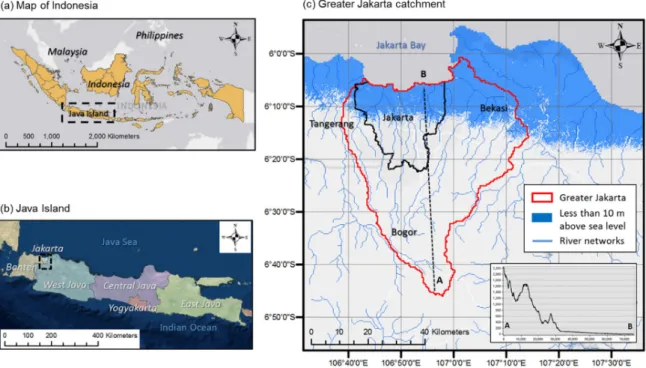
Figure 1.7 (a) Map of Indonesia; (b) map of Java Island; and (c) Greater Jakarta catchment with low-lying areas shown in blue, less than 10 m above MSL ... 10

Figure 1.8 Schematic diagram of the research ... 11

Figure 2.1 Digital surface model and digital terrain model [Asharyanto et al., 2015] ... 15

Figure 2.2 Schematic diagram of ANN layers [Haykin, 1994] ... 20

Figure 2.3 Mean seasonal surface winds (m/s) during Northeast Monsoon (top), and Southwest Monsoon (bottom), 1986-2005 ... 24

Figure 2.4 Climatological annual mean surface air temperature (°C), 1986-2005 ... 24

Figure 2.5 Climatological annual mean precipitation (mm/day), 1986-2005 ... 25

Figure 2.6 Illustration of derivation of IDF curve [Nhat et al., 2006] ... 28

Figure 3.1 Limitations of SRTM DEM on the scanning of surface [Radiomobile, 2018]... 34

Figure 3.2 Different DEMs from different sources; urban area in Nice, France; (a) satellite imagery, (b) surveyed DEM (1 m resolution), (c) TanDEM-X DEM (12 m resolution), (d) SRTM DEM (30 m resolution; publicly accessible satellite data) ... 35

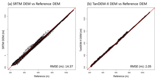
Figure 3.3 Performance of (a) SRTM DEM and (b) TanDEM-X DEM compared to surveyed/reference DEM over an urban area in Nice, France ... 35

Figure 3.4 Different DEMs from different sources; forested area in Nice, France; (a) satellite imagery, (b) surveyed DEM (1 m resolution), (c) TanDEM-X DEM (12 m resolution), (d) SRTM DEM (30 m resolution; publicly accessible satellite data) ... 36

(12)

xi

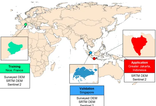
Figure 3.5 Performance of (a) SRTM DEM and (b) TanDEM-X DEM compared to surveyed/reference DEM over forested area in Nice, France ... 37 Figure 3.6 Schematic diagram of DEM improvement methodology ... 37 Figure 3.7 Different resolutions of different remote sensing data from Sentinel 2, SRTM DEM, TanDEM-X DEM and Surveyed DEM ... 38 Figure 3.8 Areas used for ANN’s training (Nice, France), validation (Singapore) and application (Greater Jakarta, Indonesia) of DEM improvement scheme ... 39 Figure 3.9 Data coverage of SRTM DEM (https://www2.jpl.nasa.gov/srtm/index.html) ... 40 Figure 3.10 Sharpness comparison between (a) SRTM DEM and (b) high-resolution DEM ... 40 Figure 3.11 SRTM DEM void filling with interpolation method; (a) satellite imagery, (b) void hole in SRTM DEM data, (c) void hole filled after interpolation using data from neighboring cells ... 41 Figure 3.12 Data coverage of TanDEM-X DEM (status as of August 2016) ... 43 Figure 3.13 Limitation of TanDEM-X DEM on water body; (a) TanDEM-X DEM, (b) SRTM DEM, (c) surveyed DEM ... 44 Figure 3.14 MSI spectral bands versus spatial resolution [Gatti and Bertolini, 2018] ... 45 Figure 3.15 Different reflectance of Sentinel 2 in different landuses; (a)-average values of reflectance from each band for different landuses, (b) standard deviation of different landuses ... 47 Figure 3.16 Standardization of different resolutions from different sources ... 48 Figure 3.17 Domain of Regional Climate Model, WRF (20 km resolution): ... 51 Figure 3.18 Comparison of climatological daily mean precipitation (mm/day; 1986-2005) (a) CHIRPS, (b) WRF/ERAI (extracted from Liu [2017]) ... 53 Figure 3.19 Comparison of climatological daily Simple Day Intensity Index of precipitation (SDII; mm/day; 1986-2005) (a) CHIRPS, (b) WRF/ERAI (extracted from Liu [2017]) ... 54 Figure 3.20 Comparison of climatological annual 95th_{percentile of precipitation (P95p; mm/day;}

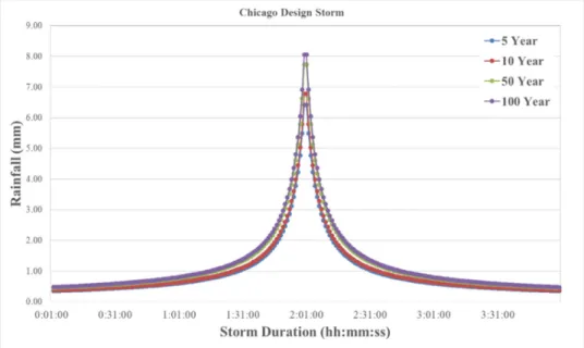
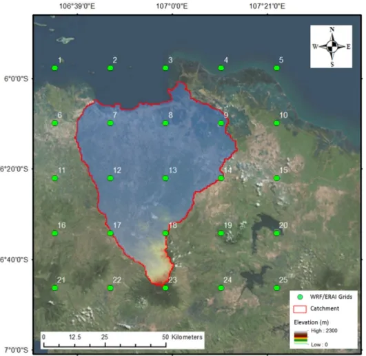
1986-2005) (a) CHIRPS, (b) WRF/ERAI (extracted from Liu [2017]) ... 54 Figure 3.21 A sample of design storm time series for 5, 10, 50 and 100 year return periods and a total duration of 4 hours ... 60 Figure 3.22 Map showing twenty-five (25) grid points of WRF/ERAI model; the color represents DEM ... 61

(13)

Figure 3.23 Volume fluxes perpendicular to element faces [DHI, 2017] ... 63

Figure 3.24 Sample of different mesh sizes in MIKE Zero Mesh Generator ... 65

Figure 3.25 Tide level setup with rainfall intensity time series ... 66

Figure 4.1 Training and test areas in Nice, France: forested areas ... 69

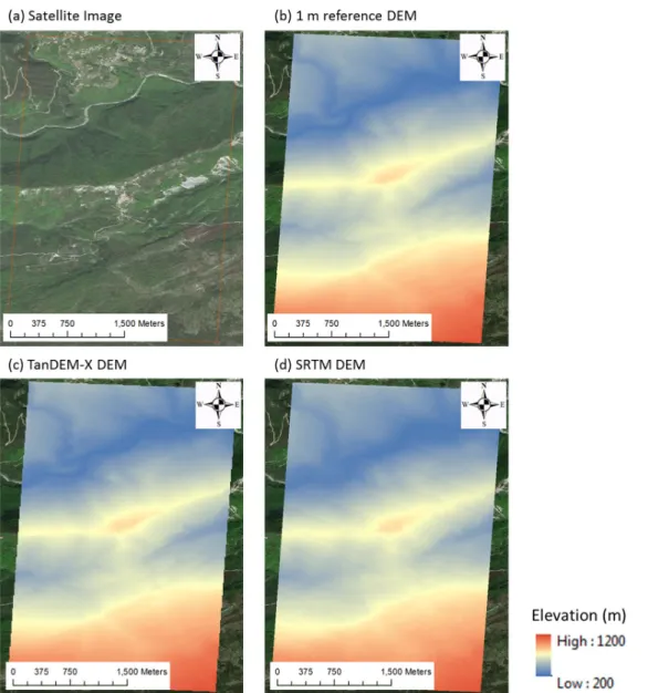
Figure 4.2 Comparisons of (a) satellite image, (b) 1 m reference DEM, (c) SRTM DEM and (d) iSRTM DEM in forested area in Nice, France... 70

Figure 4.3 Scatter plots and RMSE comparisons between (a) SRTM DEM and (b) iSRTM DEM in forested area in Nice, France ... 71

Figure 4.4 Absolute errors (a) between reference DEM and SRTM DEM; and (b) between reference DEM and iSRTM DEM in forested area in Nice, France ... 71

Figure 4.5 Training and test areas in Nice, France: dense urban areas ... 72

Figure 4.6 Comparisons of (a) satellite image, (b) 1 m reference DEM, (c) SRTM DEM, (d) iSRTM_v1 DEM, and iSRTM_v2 DEM in dense urban areas in Nice, France ... 73

Figure 4.7 Scatter plots and RMSE comparisons between (a) SRTM DEM, (b) iSRTM_v1 DEM and iSRTM_v2 DEM in dense urban area in Nice, France ... 74

Figure 4.8 Absolute errors between (a) reference DEM and SRTM DEM; (b) reference DEM and iSRTM_v1 DEM; and (c) reference DEM and iSRTM_v2 DEM in dense urban area in Nice, France ... 75

Figure 4.9 Training and test areas in Singapore: forested areas ... 76

Figure 4.10 Comparisons of (a) satellite image, (b) 1 m reference DEM, (c) SRTM DEM and (d) iSRTM DEM in forested area in Singapore ... 77

Figure 4.11 Scatter plots and RMSE comparisons between (a) SRTM DEM and (b) iSRTM DEM in forested area in Singapore ... 78

Figure 4.12 Absolute errors between (a) reference DEM and SRTM DEM, and (b) reference DEM and iSRTM DEM in forested area in Singapore ... 78

Figure 4.13 Training and test areas in Singapore: dense urban areas ... 79

Figure 4.14 Comparisons of (a) satellite image, (b) 1 m reference DEM, (c) SRTM DEM and (d) improved SRTM_v2 DEM in dense urban area in Bukit Timah, Singapore ... 80

(14)

xiii

Figure 4.15 Scatter plots and RMSE comparisons between SRTM DEM and iSRTM_v2 DEM in Urban in Bukit Timah, Singapore ... 80 Figure 4.16 Absolute errors between (a) reference DEM and SRTM DEM, and (b) reference DEM and iSRTM_v2 DEM in dense urban area in Bukit Timah, Singapore ... 81 Figure 4.17 Performance comparisons of (a) 1 m reference DEM, (b) SRTM DEM, (c) iSRTM DEM trained in Singapore and (d) iSRTM DEM trained in Nice, France: forested area ... 83 Figure 4.18 Scatter plots and RMSE comparison between (a) SRTM DEM, (b) iSRTM_v2 DEM trained in Singapore and (c) iSRTM_v2 DEM trained in Nice, France: forested area ... 84 Figure 4.19 Performance comparisons of (a) 1 m reference DEM, (b) SRTM DEM, (c) iSRTM_v2 DEM trained in Singapore and (d) iSRTM_v2 DEM trained in Nice, France: dense urban area ... 85 Figure 4.20 Scatter plots and RMSE comparison between SRTM DEM, iSRTM DEM trained from Singapore and iSRTM DEM trained from Nice, France: dense urban area ... 86 Figure 4.21 DEM comparisons of (a) 1 m reference DEM, (b) TanDEM-X DEM and (c) iSRTM_v2 DEM in Nice, France ... 88 Figure 4.22 Scatter Plots and RMSE comparisons between (a) TanDEM-X DEM and (b) iSRTM_v2 DEM trained in Nice, France ... 88 Figure 4.23 DEM comparisons of (a) 1 m reference DEM, (b) TanDEM-X DEM and (c) iSRTM_v2 DEM in Singapore ... 89 Figure 4.24 Scatter plots and RMSE comparisons between (a) TanDEM-X DEM and (b) iSRTM_v2 DEM in Singapore ... 90 Figure 4.25 Comparisons of drainage networks derived from (a) 1 m reference DEM, (b) TanDEM-X DEM, (c) SRTM DEM and iSRTM_v2 DEM: Nice, France ... 92 Figure 4.26 Comparisons of drainage networks derived from (a) 1 m reference DEM, (b) TanDEM-X DEM, (c) SRTM DEM and iSRTM_v2 DEM: Singapore ... 92 Figure 4.27 Singapore’s IDF curves with rainfall record up to 2009 (extracted from PUB, 2012) .. 95 Figure 4.28 Comparisons of IDF curves resulting from WRF/ERAI, CHIRPS and COP35 ... 96 Figure 5.1 (a) Satellite imagery of study area; (b) Jakarta Metropolitan with four areas chosen for comparisons ... 100 Figure 5.2 Comparisons between (a) satellite imagery, (b) SRTM DEM and (c) iSRTM_v2 DEM: area 1 ... 101

(15)

Figure 5.3 Comparisons between (a) satellite imagery, (b) SRTM DEM and (c) iSRTM_v2 DEM:

area 2 ... 102

Figure 5.4 Google street (a) view of circle 1 and (b) view of circle 2 in Figure 5.3 ... 103

Figure 5.5 Comparisons between (a) satellite imagery, (b) SRTM DEM and (c) iSRTM_v2 DEM: area 3 ... 104

Figure 5.6 Comparisons between (a) satellite imagery, (b) SRTM DEM and (c) iSRTM_v2 DEM: area 4 ... 105

Figure 5.7 Drainage network comparisons between SRTM (mint green) and iSRTM_v2 DEM (yellow) in (a) area 1 and (b) area 2 ... 106

Figure 5.8 WRF/ERAI grid points considered for RFA ... 107

Figure 5.9 WRF/ERAI derived IDF curves for Greater Jakarta: duration of 1 to 7 days, return periods of 50- and 100-years ... 109

Figure 5.10 (a) Different elevation ranges over Greater Jakarta and (b) longitudinal profile from point A to point B ... 111

Figure 5.11 Rainfall design storms for Greater Jakarta upstream and downstream catchments ... 112

Figure 5.12 Areas with fine and coarse meshes ... 113

Figure 5.13 Water bodies in Greater Jakarta, Indonesia ... 115

Figure 5.14 Maximum flood depths (m) of Greater Jakarta with (a) 50- and (b) 100-year return period from iSRTM_v2 DEM and (c) 100-year return period from SRTM DEM ... 117

Figure 5.15 Comparison of (a) flood footprints of 2013 Jakarta flooding; 100-year return period of flood maps from (b) iSRTM_v2 DEM; and (c) SRTM DEM ... 119

(16)

xv

TABLE OF TABLES

Table 1-1 Statistic of reported disaster between 1970 and 2009 [UNISDR, 2010] ... 4

Table 1-2 Climate information of Jakarta [Sun et al., 2014] ... 9

Table 2.1 Classification of Flood models [Neelz and Pender, 2009; Pender, 2006] ... 30

Table 3.1 TanDEM-X DEM product overview [Wessel et al., 2016] ... 42

Table 3.2. Sentinel 2 spectral bands [Gatti and Bertolini, 2018] ... 45

Table 3.3 Sentinel 2 product processing levels ... 46

Table 3.4. Average of reflectance values with different landuses ... 47

Table 3.5 Artificial Neural Network layers ... 49

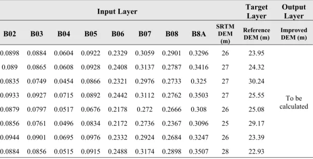
Table 3.6 Input, Target and Output Layers in Artificial Neural Network (example) ... 50

Table 3.7 Basic characteristic of ERAI and WRF/ERAI data ... 52

Table 3.8 Critical values for the discordancy statistic Di [Hosking and Wallis, 1997] ... 56

Table 4.1 Summary table of the performances of iSRTM DEM in Nice, France ... 75

Table 4.2 Summary table of the performances of iSRTM DEM in Singapore ... 81

Table 4.3 Summary table of performances of iSRTM DEMs trained in Nice, France and trained in Singapore and applied to test areas in Singapore ... 86

Table 4.4 Summary of performances of various scenarios ... 93

Table 4.5 Extreme rainfall intensities resulting from WRF/ERAI, CHIRPS and COP35 ... 96

Table 5.1 Summary table of the data obtained for study area ... 99

Table 5.2 Discordancy (Di) measure of study area ... 108

Table 5.3 Heterogeneity (H) measure of study area ... 108

Table 5.4 Chicago Design Storm method fitted equations for Greater Jakarta IDF curves ... 110

Table 5.5 Rainfall intensity (mm/hr) derived from WEF/ERAI for different return periods of 1 to 7 days storm durations ... 110

Table 5.6 Parameters to calculate the Time of Concentration (TC) ... 112

(17)

(18)

xvii

LIST OF ABBREVIEATION

ACCESS1.3 Australian Community Climate and Earth-System Simulator AI Artificial Intelligence

AMR Annual Maximum Rainfall ANN Artificial Neural Network

APHRODITE Asian Precipitation - Highly-Resolved Observational Data Integration Towards Evaluation

ASEAN Association of South East Asian Nations

ASTER Advanced Spaceborne Thermal Emission and Reflection Radiometer BCA Building and Construction Authority

BRDF Bidirectional Reflectance Distribution Function CDF Cumulative Distributed Function

CFL Courant-Friedrich-Lewy

CHIRPS Climate Hazards Group InfraRed Precipitation with Station COP35 35 rainfall stations, in Code of Practice

CRU Climate Research Unit DEM Digital Elevation Model

DLR German Aerospace Center (German: Deutsches Zentrum für Luft- und Raumfahrt e.V.)

DSM Digital Surface Model DTM Digital Terrain Model

ECHAM6 European Centre HAMburg Model

ECMWF European Centre for Medium-Range Weather Forecasts EROS Earth Resources Observation and Science

ESA European Space Agency

ESRI Environmental System Research Institute GCM Global Climate Model

GDEM Global DEM

GEV Generalized Extreme Value GIS Geographic Information System GMES Global Monitoring for Environment and Security GPS Global Positioning System

GPU Graphical Processing Units GTM Global Tide Model

IDF Intensity-Duration-Frequency InSAR Interferometric Synthetic Aperture Radar iSRTM DEM Improved SRTM DEM

(19)

L-CV L-Coefficient of Variation

LiDAR Laser Imaging Detection and Ranging LM Levenberg-Marquardt

METI Ministry of Economy, Trade, and Industry MIKE21FM MIKE21 Flow Model Flexible Mesh

MIROC5 Model for Interdisciplinary Research on Climate MSI Multispectral Instrument

MSL Mean Sea Level

NASA National Aeronautics and Space Administration NBAR Nadir BRDF Adjusted Reflectance

NDWI Normalised Difference Water Index NIR Near Infrared

NOAA National Oceanic and Atmospheric Administration NSI National Space Institute

OSM Open Street Map P95p 95th Percentile of Precipitation

PDF Probability Density Function PUB Public Utility Board

RCM Regional Climate Model

RCP Representative Concentration Pathway RFA Regional Frequency Analysis

RMSE Root Mean Square Error

SDII Simple Day Intensity Index SRTM Shuttle Radar Topography Mission SWIR Short Wave Infrared SWMM Storm Water Management Model TC Time of Concentration

THB Thai baht

TOA Top-Of-Atmosphere USGS United States Geological Survey VNIR Visible and Near Infrared

WRF Weather Research and Forecast WRF/ERAI WRF driven by ERA-Interim

(20)

1 Introduction

1.1 Background

Flooding is known as one of the most devastating and costliest global phenomena that can seriously disrupt transport and communication, severely damage properties, and cause devastated economic and human losses. Flooding is likely to be even further worsened in the future with changing climate. With clearly increasing global temperature, extreme weather events have been recorded; in Southeast Asia alone in recent years, these extreme events range from typhoon Haiyan (the highest category 5) in 2013, heavy rainfalls (and hence flooding in Jakarta 2007, Hanoi 2008, Bangkok 2011) to resulting landslides. Rainfall events with both higher intensity and frequency have been observed and are likely to continue. A warmer atmosphere is expected to accelerate the hydrological cycle due to the higher humidity content.

In late June through mid-July 2018, heavy downpours in Japan, a country highly ranked in disaster preparedness, resulted in severe floods and landslides. 225 people were confirmed dead in the affected areas, and economic losses reached an estimated US$ 3.66 billion [Sim, 2018]. Despite the efforts of many international organizations and countries, these catastrophes continue to occur at alarming rate. In Southeast Asia this is due to the rapid urbanization (hence, increasing migration into the urban areas for economic reasons), poor urban planning and enforcement of storm drainage network designs and maintenance works.

Insurance Information Institute ( https://www.iii.org/fact-statistics/facts-statistics-global-catastrophes) showed insightful statistics on various world natural catastrophes by type of events in 2017, and by continent as shown in Figure 1.1 (a) and (b) respectively. Figure 1.1 (a) showed the number of events, fatalities and insured losses mainly caused by meteorological and hydrological events (about 80 % combined) while Figure 1.1 (b) clearly showed how vulnerable Asian continent is in the number of events (44 %), fatalities (65 %) and insured losses (2 %). The message is very alarming for Asia as the vulnerability is high and yet the insured losses are extremely low compared to their North American counterparts. Insurance Information Institute gave further breakdown on world weather-related catastrophes by type of events in 2017, and by continent as shown in Figure 1.2 (a) and (b) respectively. Figure 1.2 (a) showed the number of

(21)

events (51 %) and fatalities (75 %) caused by hydrological events (flood, mass movement) dominated; the corresponding insured losses, however, was just 1 %. The statistics for Asia was again most alarmingly vulnerable: the number of events was 41 %, fatalities 66 %, and yet the insured losses only 2 %; note that most likely the main portion of the insured losses is in more developed countries such as Japan, Korea, and Singapore. Southeast Asian countries are indeed very vulnerable.

Figure 1.1 World natural catastrophes by (a) type of event and (b) continent in 2017 [III, 2018]

(22)

Figure 1.2 World weather-related catastrophes by (a) type of event and (b) continent in 2017 [III, 2018]

Southeast Asia comprises of 11 nations - Indonesia, Malaysia, Singapore, Vietnam, Brunei, Laos, Myanmar, Philippine, Thailand, Cambodia and Timor Leste. This region covers an area of about 4.5 million km2_{which is 3 % of the earth’s land area. Its population is more than 641 million which} is about the 8.5 % of world’s population. The economic growth rate of Southeast Asia is the fastest growth in the world since 1990. With abundant resources and high population growth, the overseas investments concentrate in rapidly developing coastal megacities. However, Southeast Asia is geographically located in one of the most disaster-prone regions of the world; many countries in the region have a history of devastating disasters that have caused colossal economic and human losses. According to ASEAN (Association of South East Asian Nations) Disaster Risk Management Initiative, flood is the most reported disaster in ASEAN countries between 1970 and

(23)

2009, as listed Table 1-1. Out of all reported disasters, 36 percent were floods, 32 percent were cyclonic storms [UNISDR, 2010].

Indonesia, one of the most vulnerable countries to natural disasters, experienced in year 2018 almost 2,000 natural disasters (tsunami, earthquake and flooding) which claimed nearly 4,000 lives and displaced around 3 million people. As recent as in December 2018, Sunda Strait tsunami, triggered by a volcanic activity on the island of Anak Krakatoa, caused 429 deaths and 1,485 injured [Renaldi and Shelton, 2018].

The damage of natural disasters is expected to become more severe in the future due to rapid developments and population growth over the study region compounded with climate change. Challenges faced by ASEAN are huge. ASEAN needs to incorporate future potential risks into disaster risk reduction.

Table 1-1 Statistic of reported disaster between 1970 and 2009 [UNISDR, 2010] Disaster type No. of disasters /year Total no. of deaths Deaths/ year Relative vulnerability (deaths/year/million) Average annual economic loss ($ million) Flood 10.85 17,800 445.0 0.75 312.1 Storm 9.65 184,063 4,601.6 7.76 339.4 Epidemic 2.28 7,294 182.4 0.31 - Landslide 2.05 5,058 126.5 0.21 4.4 Forest Fire 0.45 310 7.8 0.01 511.9 Drought 0.98 1,337 33.4 0.06 45.8 Tsunami 0.15 92,021 2,300.5 3.88 214.2 Volcano 1.33 1,380 34.5 0.06 32.1 Earthquake 2.58 105,735 2,643.4 4.46 243.9

Focusing further on Southeast Asia, a study of Yusuf and Francisco [2009], relevant to present conditions, highlighted the climate hazards over domain using a multi climate index; the study conducted a vulnerability mapping based on tropical cyclones, floods, landslides, droughts, and sea level rise. Figure 1.3 and Figure 1.4 focus on the overall climate hazard and the annual flood frequency maps for Southeast Asia. Figure 1.3 showed, for example, how vulnerable the Philippines is; its vulnerability is mainly caused by destructive typhoons which hit the Philippines about 5 times annually. Figure 1.4 showed, for example, the vulnerability of the city of Jakarta (on Java island of Indonesia) to floods.

(24)

Figure 1.3 Multiple climate hazard map of Southeast Asia [Yusuf and Francisco, 2009]

Figure 1.4 Annual flood frequency map of Southeast Asia [Yusuf and Francisco, 2009]

To briefly highlight the severity of floods in Southeast Asia in recent years, two countries, Thailand and Indonesia, are singled out here. In July – Dec 2011, Central and Northern Thailand received 300 to 500 mm (that is about 3 times) more rainfall than the normal condition as the Asian monsoon

(25)

started early with an extraordinary heavy rainfall [Bevere et al., 2012], as shown in Figure 1.5. Duration of flooding was 175 consecutive days. It resulted in 815 deaths and affected more than 13.6 million people. With many industrial areas severely affected, [Bhoochaoom and Dixon, 2012] estimated the total damage and economic losses of about Thai Baht (THB) 1.43 trillion (US$ 46.5 billion).

Figure 1.5 Thailand Flood in July to December 2011 [Bangkokpost, 2012]

In January – February 2007 torrential rains pounded Jakarta, the capital city of Indonesia. This caused floods that buried 36 % of the city under as much as 5 m in some areas, affected 2.6 million people, and forced 340,000 people to flee their home, as shown in Figure 1.6. Over 70 people died and outbreaks of disease affected over 200,000 people, with losses estimated at US$ 900 million. Jakarta’s notorious subsidence, estimated at 7.5 cm/year, worsens the flooding during heavy rainfall combined with high tide. This will be even of greater concern with climate change which projected increasing rainfall intensity and rising sea level.

(26)

Figure 1.6 Jakarta Flood in January 2007 [Floodlist, 2008]

1.2 Gaps in Flood Analysis

Developed countries apply, for example, sophisticated rainfall nowcasting and forecasting, well calibrated and validated flood models, and flood early warning systems to disseminate anticipated water levels in the river/stream networks and low lying areas, and thus, to minimize damages/losses caused by floods. However, developing countries may not have enough information to solve the aforementioned issues due to its economic and technical constraints. Effective preventive and mitigation measures can only be undertaken when good quality data (e.g. Digital Elevation Model (DEM) and rainfall records) are available for flood model.

There are several well established numerical flood models, such as SWMM [Rossman, 2010], SOBEK [Deltares, 2019] and MIKE Flood [DHI, 2017]. In principle, the governing equations of these models are the same, St. Venant and Navier-Stokes equations, coupled to various sub-components (infiltration, evapotranspiration, etc.), and solved by different numerical schemes. Challenges in developing countries are, among others, limited project funding to acquire the

(27)

aforementioned good quality, high temporal resolution and long rainfall record, and high spatial resolution and high accuracy DEM; their availabilities are often even doubtful.

In recent years, there is a neologism, called ‘the flood of Big Data’, which means huge data publicly accessible so people can develop immense opportunities in various ways. Remote sensing, as an example, is the process of detecting and monitoring the physical characteristics of an area by measuring its reflected and emitted radiation at a distance from the targeted area. This technology has been used, for example, in taking images on the earth’s surface, tracking clouds to predict the weather, tracking the growth of an area and changes in landuses etc.

This study focuses on two important input data required in flood modelling and analysis. They are high accuracy DEM and a long rainfall record. Remote sensing data and an artificial intelligence technique, Artificial Neural Network (ANN) are proposed to significantly improve the original remote sensing DEM data, for areas where high spatial resolution and high accuracy DEM is not available. For areas where observed rainfall data are either not available or not sufficiently long, the study proposes rainfall proxy products from various gridded observation data such as Climate Hazards Group InfraRed Precipitation with Station (CHIRPS), Climate Research Unit (CRU), Asian Precipitation - Highly-Resolved Observational Data Integration Towards Evaluation (APHRODITE) or rainfall outputs from a Regional Climate Model (RCM). The question remains how to assess flood risk in the region of interest where the aforementioned data are not available or sufficient. This study will offer (1) a methodology to derive improved DEM from publicly accessible remote sensing data, and (2) an approach to select a highly accurate rainfall proxy, from a RCM, required to construct the much needed Intensity-Duration-Frequency (IDF) curves for flood model and analysis.

(28)

1.3 Study Region – Greater Jakarta, Indonesia

As shown in Figure 1.4 and Figure 1.6, Java Island is vulnerable to flooding in Southeast Asia. Java Island is one of the large islands and most densely populated. More than half of Indonesia’s 226 million populations live in Java (141 million in 2014 Census). The island also hosts major industrial complexes.

Jakarta, a capital city of Indonesia, is located on the northwest coast of Java Island, at the mouth of the Ciliwung River on Jakarta Bay. Jakarta has a land area of about 660 km2_{with population} over 10 million [JakartaOpenData, 2015]. There are 13 main rivers flowing through the city and its vicinity. The longest river is the Ciliwung River. The climate of Jakarta is tropical wet and dry; the rainy season in Jakarta starts in December and ends in March. The rainfall intensity often reaches its peak in January or February (Table 1-2). Jakarta suffers from massive flooding almost yearly mainly due to high rainfall intensities, low lying areas and poorly managed drainages. In 2007, approximately 70 % of Jakarta’s area was flooded with water depths up to 4 meters. Area of the catchment contributing water to Jakarta Bay is about 2,976 km2_{(hereafter referred as Greater} Jakarta).

Table 1-2 Climate information of Jakarta [Sun et al., 2014]

Month Jan Feb Mar Apr May Jun Jul Aug Sep Oct Nov Dec Year

Average High (C°) 31.5 32.3 32.5 33.5 33.5 34.3 33.3 33.0 32.0 31.7 31.3 32.0 32.6 Average Low (C°) 24.2 24.3 25.2 25.1 25.4 24.9 25.1 24.9 25.5 25.5 24.9 24.9 24.8 Humidity (%) 85 85 83 82 82 81 78 76 76 77 81 82 81 Rainfall (mm) 389.7 309.8 100.3 257.8 139.4 83.1 30.8 34.2 30.0 33.1 175.0 123.0 1706.2 Although there are many steep mountains in the upstream of Greater Jakarta, most of areas near to the coastal areas are quite flat and less than 10 m above Mean Sea Level (MSL), Figure 1.7 showed (a) map of Indonesia; (b) map of Java Island; and (c) Greater Jakarta with low lying areas along the coast. Figure 1.7 (c) showed also a longitudinal profile from the upstream point A and downstream point B; it shows drastic elevation changes from mountainous (A) to low lying coastal areas (B). This clearly implies that the low lying areas are prone to floods. Despites considerable flood risk management system introduced in the past decades, the flood impacts have worsened;

(29)

the main reasons are (1) rapid urbanization with not much of urban planning; (2) poor law enforcement on drainage maintenance (e.g. garbage dumping in rivers/canals). This study provides a baseline of flood risk mapping over Greater Jakarta with innovative cost-effective technology.

Figure 1.7 (a) Map of Indonesia; (b) map of Java Island; and (c) Greater Jakarta catchment with low-lying areas shown in blue, less than 10 m above MSL

1.4 Research

Motivations

To implement flood adaptation measures, it is imperative to couple topographical, hydrological and hydraulic understanding with model analysis. High spatial resolution and high accuracy DEM, and high temporal resolution and long rainfall records are important in flood hazard assessment using numerical model. Challenges in developing countries, such as Indonesia, are obtaining: (1) high accuracy DEM which is very costly and time consuming to acquire; and (2) good quality and long rainfall record required to derive Intensity-Duration-Frequency curves, design curves for drainage.

Figure 1.8 showed the schematic diagram of the process how the most relevant data for the flood simulations and analysis are cost effectively obtained. The research motivations and processes are summarized as follows.

(30)

1. DEM data from a publicly accessible remote sensing satellite will be selected and used to train an ANN to improve the quality of the remote sensing DEM. In the training of ANN, high quality observed DEM is the key leading to a well-trained ANN. The trained ANN will then be ready to efficiently and effectively generate high quality DEM, at low cost, for places where DEM data is not available.

2. Rainfall data, resulting from a high spatial resolution Regional Climate Model, RCM, will first be extracted, analyzed, and compared with regard to accuracy with good quality observed rainfall data of gauged catchments. The comparisons are performed, among others, on their IDF curves which are the essential design curves for storm drainage. After checking its high accuracy, the rainfall data (from the RCM) for an ungauged catchment will be extracted and readily used as proxies to derive the IDF curves for that ungauged catchment.

3. Data from the aforementioned two steps are then used as input to a widely used numerical flood model to generate flood data and the much needed flood map of various return periods. Policy makers will then be well informed about anticipated flood prone areas and flood extents to come up with best flood preventive and mitigation measures.

(31)

1.5 Structure

of

Thesis

This thesis consists of six chapters. A brief description of each chapter is as follows:

 Chapter 1 presents the background of the study, gaps, study areas, research motivations, and structure of thesis.

 Chapter 2 presents a series of literature reviews relevant to (1) Digital Elevation Model (DEM): satellite data and multispectral imagery, and artificial neural networks with which cost effective DEM are derived; (2) Proxy for high temporal resolution and long rainfall data record: Regional Climate Model data (rainfall data in particular), and regional frequency analysis with which proxy rainfall data are then used to derive Intensity-Duration-Frequency curves; and (3) Numerical models: which assesse flood prone areas and flood extents.

 Chapter 3 presents (1) the proposed methodology to improve publicly accessible DEM; and (2) the approach to select proxy rainfall data from downscaled climate model; suitability of data from various grid points will be checked using regional frequency analysis for derivation of the IDF curves which are relevant to storm drainage designs and flood analysis.

 Chapter 4 demonstrates proof of concepts laid out in Chapter 3. It first shows the performance of the improved DEM through comparisons with their observed counterparts (in Nice, France, and in Singapore). It then presents the accuracy of derived high temporal and long rainfall proxy data using IDF curves comparison between model output and rainfall station data.

 Chapter 5 presents the application of the aforementioned methodologies on Greater Jakarta (Indonesia) where both high resolution DEM and rainfall data are not available or not easily obtained. Flood map of two return periods (50- and 100-Years) are presented and compared with 2013 Jakarta flood footprint.

 Chapter 6 summarizes and highlights the main results for each objective of the study; concludes the findings; and makes recommendations for future studies.

(32)

2 Literature

Review

2.1 Introduction

This chapter reviews literatures relevant to remote sensing technology, artificial neural network, climate models and numerical flood modelling. To assess flood hazards, a series of data/information, such as digital elevation model and rainfall data, are required. In many countries, the developing ones in particular, these data are not readily available because (1) the high cost of the measurement and proper related tasks, or (2) no data record or data confidentiality. Hence publicly accessible remote sensing data, e.g. digital elevation model, are often the only option. However, the quality of remote sensing data, in some cases, requires further enhancement. This study considers Artificial Neural Network (ANN), a part of artificial intelligence technology or machine learning, to improve the accuracy of remote sensing data. Rainfall data in many developing countries, aside from data quality, are often of short record duration or not in existence. In areas of interest such as Greater Jakarta, Indonesia, this poses difficulty to engineers to arrive at appropriate design curves for drainages. As mentioned in Chapter 1, for Greater Jakarta, this study considers rainfall data, derived from a Regional Climate Model (RCM) driven by reanalysis data, as proxies. This information is parts of the essential input data for numerical flood model.

2.2 Remote Sensing Technologies

Remote sensing is the process of collecting information about an object area or phenomenon without physical contact [Navalgund et al., 2007]. It has two aspects which are intimately linked with each other: the technology of obtaining the data through a device whose location is at a distance from the object, and analysis of the data for the interpretation of the physical objects [Gupta, 2018]. Going by the aforementioned definition various techniques of collecting the data where the object and sensor are not in contact with each other can be classified as remote sensing, for example photography, infrared, radiometers, radar (i.e. an object-detection system that uses radio waves to determine the range, angle, or velocity of objects) and Laser Imaging Detection and Ranging (LiDAR) (i.e. a surveying method that measures the illuminating target with pulsed laser light and the reflection of pulses with a sensor). Remote sensing can also be used as the technique

(33)

of sensing the earth’s surface from space by making use of the properties of electromagnetic wave emitted, reflected or diffracted by sensed objects, for the purpose of improving natural resource management, landuse and the protection of the environment.

Remote sensing has mainly evolved from the various methods of aerial photography and interpretation of the photos. It is a comparatively young discipline of science which has significantly grown over the past five decades. It has effectively improved human’s ability to explore resources, map and monitor the Earth’s environment globally and locally [Lillesand et al., 2015; Rencz et al., 1996; Thenkabail, 2015]. Earth observation is the main application of remote sensing. Various types of earth observations are listed below [Entwistle et al., 2018; Gupta, 2018;

Kugler, 2012].

 Weather forecasting

 Measuring land surface and mapping  Tracking of biodiversity and wildlife trends

 Tracking of landuse changes (such as deforestation)

 Monitoring and responding to natural disasters, including forest/bush fires, floods, earthquakes and tsunamis

 Managing natural resources, such as energy, freshwater and agriculture  Addressing emerging diseases and other health risks

 Predicting, adapting to and mitigating climate change.

Systematic and concise timelines of key developments in platforms and sensors for earth observations are well summarized in Green and Jackson [2009]. The first photo of the earth from the space was transmitted by Explorer-6 in 1959. It provided an orbital photography with the help of an unmanned camera. The Gemini mission of 1965 gave a number of vertical, stereo, oblique photographs of good quality. This demonstrated the potential of remote sensing techniques in the exploration of the resources on the earth. Later on, the experiments of the Apollo program included the coverage of the earth by multispectral 70-mm format photography and stereo vertical photography. The series of experiments on the photography led to the development of unmanned space orbital sensors.

(34)

2.2.1 Digital

Elevation

Models

Spaceborne radar or airborne laser scanning are widely applied to retrieve data on topography that is used to develop the Digital Elevation Model (DEM) [Mirosław-Świątek et al., 2016; Rodriguez

et al., 2006; Zhang and Montgomery, 1994]. A DEM can be used to depict the terrain of the earth

and is an organised array of the numbers which represent the elevations of spatial distributions above an arbitrary datum. The primary principle of a DEM is to describe the elevations of various points in a given area in digital format. The term DEM is usually applied to land surface topography, but it is a general term which is used to depict the spatial patterns of various surfaces e.g. surface water, ground surface, canopy, etc. Digital Surface Model (DSM) and Digital Terrain Model (DTM) are the two other terms which are frequently used for the ground terrain. DTM is referred as to the Earth terrain i.e. bare ground while DSM includes objects on ground like the buildings and trees, Figure 2.1.

Figure 2.1 Digital surface model and digital terrain model [Asharyanto et al., 2015]

A DEM can be obtained from various types of data sources. Traditionally, the ground survey data is most accurate but is also most expensive depending on the sampling density [Bartosh, 2012]. Recently the airborne laser scanning seems to be the most accurate method with the highest sampling density. It can record both object on surface and ground surface so that the elevation data is considered as the DSM [Asharyanto et al., 2015; Mirosław-Świątek et al., 2016]. Spaceborne interferometric radar system is a cost-effective technique to obtain the land cover and terrain data. A DEM can also be derived from radar satellite such as Shuttle Radar Topography Mission (SRTM DEM) [Hensley et al., 2000; Jacobs et al., 2001; Kim et al., 2019; Rosen et al., 2001], Advanced Spaceborne Thermal Emission and Reflection Radiometer (ASTER) [Reuter et al., 2009;

(35)

SRTM DEM is an international joint project to collect three-dimensional digital mapping of over 80 % of the Earth’s surface (between 60° N and 56° S) and it is available at no cost [USGS, 2000]. 3 arc-second resolution is available since 2005 and 1 arc-second resolution for globe is available after 2015. The performance requirements for the SRTM DEM data are such that the linear vertical absolute height error shall be less than 16 m and the relative height error shall be less than 10 m, for 90 % of the data [Rodriguez et al., 2006]. It should be noted, however, that its accuracy is limited to Root Mean Square Error (RMSE) of approximately 14 m over Singapore’s forest areas due to C-band wavelengths (λ ≈ 5.6 cm) that does not adequately penetrate the vegetation canopy [Wendi et al., 2016]. Thus, the elevation in vegetation area presents an intermediate height between top of canopy and the bare surface. Also, due to its coarse resolution (~ 30 m since 2015; ~ 92 m prior to 2015), it does not present precise urban characteristics.

The Global DEM (GDEM) is obtained from ASTER data, a product of Japan’s Ministry of Economy, Trade, and Industry (METI) and USA’s National Aeronautics and Space Administration (NASA) [Tachikawa et al., 2011]. The ASTER GDEM produces a high resolution global digital elevation model, with 30 m spacing (1 arc second). Several literatures compared DEMs originated from SRTM DEM and ASTER DEM. Guth [2010] compared the data at 52 locations in Europe and North America and found that ASTER data was similar to SRTM DEM but about 20 % of ASTER data have anomalies that degrade its use for most applications. Li et al. [2012] conducted the evaluation of ASTER DEM, using GPS (Global Positioning System) as benchmarks, and SRTM DEM in China and concluded that ASTER DEM data requires further improvements as it appeared to overestimate the SRTM DEM data of the study area.

Graf et al. [2018] assessed the DTM for hydrogeomorphological modelling in small Mediterranean

catchments, including SRTM DEM, ASTER DEM and LiDAR datasets. The RMSE results of the vertical accuracy show that SRTM DEM and ASTER DEM have differences of 6.98 m and 16.10 m respectively over the study areas due to systematic distortions and coarse horizontal resolution. The authors concluded that these limitations should be carefully considered when applying the data for numerical modelling.

Abily et al. [2015] developed a runoff model using very high resolution DSM. Two types of DSM

data were used as topography data in the model and compared to LiDAR data only, and the combination of photogrammetric and LiDAR. Both data were able to capture the main buildings; but small buildings were not captured by LiDAR data. This resulted in significant differences in

(36)

the flood map outputs. The authors recommended that fine-tuning topographic data is necessary for high resolution flood modelling.

The German Aerospace Center (DLR) has been operating Germany’s first twin Synthetic Aperture Radar (SAR) satellites, TerraSAR-X and TanDEM-X DEM, to generate an updated global DEM shich has a spatial resolution of 0.4 arc-second (≈ 12 m) with 2 - 4 m in relative vertical accuracy [Wessel et al., 2016]. Gruber et al. [2012] compared TanDEM-X DEM data against ground control points in Germany and US; they found that the absolute height errors are between 1 and 2 m. The elevation of TanDEM-X DEM is much more accurate than SRTM DEM; but TanDEM-X DEM data is not free (https://tandemx-science.dlr.de/). More detailed comparisons are given in Chapter 3.

In this study, SRTM DEM is selected to develop the DEM improvement scheme. Very high accuracy surveyed DEM is also used, in the DEM improvement scheme, for the Artificial Neural Network (ANN) to learn the patterns.

2.2.2 Multispectral

Imagery

Multispectral imagery is produced by the sensors which measure the reflected energy within several specific bands/sections of the electromagnetic spectrum. It can be defined as “acquisition of images in hundreds of contiguous, registered, spectral bands such that for each pixel a radiance spectrum can be derived” [Goetz et al., 1985]. The multispectral sensors have 3 to 10 different measurements of the band in each pixel of the images. Various earth observation satellites are being used to capture the images of the earth. Such satellites are called imaging satellites which are normally operated by commercial companies and governments around the world [Nelli et al., 2018]. Over the years many countries have launched different satellites to acquire the images of the earth.

LANDSAT program is a network of the remote sensing satellites supported by NASA which provides repetitive acquisition of moderate-resolution multispectral data of the earth's surface on a global basis. The older satellites were gradually replaced by the more advanced and modern satellites. Presently, Landsat-7, launched in 1999, and Landsat-8, launched in 2013, are in operation. The information obtained from Landsat images meet the diverse needs of business, education, science, national security and the government. The data from the Landsat spacecraft

(37)

represents the longest record of the earth's continental surfaces observed from space. It is a file unmatched in quality, detail, coverage, and value. Landsat is the only source of global, calibrated, moderate spatial resolution measurements of the earth's surface that are preserved in a national archive and freely available to the public [Wulder et al., 2016]. The main objectives of Landsat 8 is to succeed the mission of Landsat 4, 5, 6 and 7 and to build, periodically refresh a global archive of sunlit, substantially cloud-free land images. Landsat 8 offers the features of data continuity, free standard data products, global survey mission, radiometric and geometric calibration, and responsive delivery.

Sentinel 2 is also an earth observation mission which was developed by the European Space Agency (ESA) as a part of Copernicus Programme to perform terrestrial observations in support of services such as forest monitoring, land cover changes detection, and natural disaster management [Drusch et al., 2012]. It consists of twin polar orbiting satellites in the same orbit with a phase difference of 180 degrees with each other. The satellites were built by Airbus Defence Space, Sentinel-2A and Sentinel-2B, with two additional satellites being constructed by Thales Alenia Space. The Sentinel-2A multispectral instrument (MSI) obtains the reflective wavelength of the multispectral observations with directional effects caused because of the reflectance anisotropy of the surface [Roy et al., 2017]. Roy et al. [2017] examined the magnitude of Sentinel-2A view zenith bidirectional reflectance distribution function (BRDF) effects observed for a large amount of data acquired over two 10-day periods across southern Africa acquired in the solar principal and orthogonal planes. An empirical c-factor approach was published that provides consistent Landsat view angle corrections to provide Nadir BRDF Adjusted Reflectance (NBAR) [Roy et al., 2016]. Future Sentinel-2 and Landsat satellites may provide sufficient cloud-free observations to enable reliable local parameterization of the surface reflectance anisotropy over Sentinel-2 observation conditions.

The multispectral imagery can be used for land use classification, for seasonal monitoring, agricultural and environmental application [Andres et al., 1994; Ashish et al., 2009; Moody et al., 2014; Pande et al., 2018]. Using different reflectance values from different land use types, the area can be classified by clustering and machine leaning methods. Kim et al. [2018] analyzed the different reflectance of Sentinel 2 with different land uses. The reflectance of Short Wave Infrared (SWIR) bands (Bands 6-8) in forest areas is higher than that in urban areas; on the other hand, the reflectance of Near Infrared (NIR) bands (Bands 2-5) in urban areas is higher than that in forest

(38)

areas. These different characteristics at each band help to classify land use in ANN as input nodes. These characteristics have been fully utilized for this study to generate the improved SRTM DEM using both multispectral imagery and ANN.

2.2.3 Artificial

Intelligence

Artificial Intelligence (AI) is the recreation of human intelligence processes by machines, especially computer systems. These processes include learning (the acquisition of information and rules for using the information), reasoning (using the rules to reach approximate or definite conclusions), and self-correction [Axelberg, 2007].

In 1955, John MaCarthy, considered as the founder of AI, was the first person to introduce the term AI as to develop the machines that behave as though they were intelligent. Perception, learning, reasoning, problem-solving and language-understanding are the main components of AI [Andresen, 2002; McCarthy, 1956]. Some specialized areas of AI are game playing, expert systems, natural language processing, neural networks, and robotics etc. The advantages of AI, among others, are:

 It can take on stressful and complex work that humans may struggle/cannot do.  It can complete a task faster than humans can.

 It can be used for discovering unexplored things.  It yields less number of errors and, thus, less defects.  It is more versatile when compared to humans.

ANN is one of the machine learning systems to achieve AI. ANNs apply mathematical learning algorithms which are simulated by properties of the biological neural networks. ANNs are loosely based on biological neural networks in such a way that they are implemented as a system of interconnected processing elements, sometimes called nodes, which are functionally analogous to biological neurons. The connections between distinct nodes have numerical values, called weights, and systematic altering of these values will give the ability to approximate the desired function [Gurney, 2014]. The characteristics of ANNs [Kumar and Iyer, 2010; Sarve et al., 2015] are:

(39)

 It can learn from the examples so that the ANN architectures can be trained with established examples of a problem before they are tested for their inference abilities for unknown instances of the problem. This helps in the identification of new objects which are not trained previously.

 It has generalization ability which helps predict the new outcomes based on the previous outcomes.

 The system can extract important features from incomplete, partial or noisy patterns. The ANN is formed in three layers: input layer, hidden layer and output layer. The input layer has input neurons that transfer information via synapses to the hidden layer, and similarly the hidden layer transfers this information to the output layer via additional synapses. The synapses store values referred to as weights that help them to control the input and output to different layers. Figure 2.2 showed the schematic diagram of ANN.

Figure 2.2 Schematic diagram of ANN layers [Haykin, 1994]

Each node within the network takes several inputs from alternative nodes and determines one output based mostly on the inputs and also the association weights. The network is able to converge to the optimal target function by the alteration in the weights systematically. Initially random values are assigned to weights and the network has to be trained to find the optimal weights. To achieve this the first output of the neural network has to be compared to the desired output, error is first determined; using this error the weights of the network are adjusted proportional to their

(40)

contribution to the error in the output using back-propagation algorithm [Rosenblatt, 1961; Widrow

and Hoff, 1962]

Together with the aforementioned characteristic of ANN, it has now been applied to system identification and control, quantum chemistry, game playing and decision making, pattern and sequence recognition, medical diagnosis and data mining. There are some applications of ANN in pattern recognition of remote sensing data.

The classification of images based on ANN uses a non-parametric path making it easy for the incorporation of the supplementary data while classifying so that the accuracy of the classification process is improved [Abburu and Golla, 2015]. In the training phase the ANN gains the information about the regularities which is present in the training data and then it will construct the rules which can be extended to the unknown data [Foody, 1999]. The main advantage of using ANN is that it can learn and generalize from inputs to produce a meaningful solution even when the input data contain errors or is incomplete. In the case of complex classification processes ANN algorithms are highly efficient [Luk et al., 2000].

Kawabata and Bandibas [2009] utilized the ANN to generate the landslide susceptibility map

using landslide data from an event of earthquake and a DEM derived from ASTER images. The ANN was trained using six geomorphic and geologic factors to produce the landslide hazard index map. The ANN was able to model the relationship between landslide occurrence and the factors.

Sun et al. [2016] applied the ANN to predict the ground water table in a freshwater swamp forest

of Singapore. Unlike the physical modelling, the ANN-based approach did not require explicit characterization of the physical properties, or accurate representation of the physical parameters; it simply determined the system patterns based on the relationships between inputs and outputs mapped in the training process. The surrounding reservoir levels and rainfall information up to the immediate past 7 days were used as input in ANN. The forecast of the ground water table showed higher accuracy, as expected, for 1 day than for 7 days. The performance of longer lead-days results might be further improved if more variables, such as evapotranspiration, can be made available in the training of ANN process.

This study makes use of the strength of ANN in pattern recognition and classification to derive more accurate DEM. The ANN is able to classify the areas based on their reflectance values and identify the general error pattern, and reduce the errors between elevations of SRTM’s DEM and reference DEM for different land uses from training process.

(41)

2.3 Downscaled Climate Model

Downscaling is the process of deriving the climate projections to scales which the decision makers require. The spatial scale, for dynamical downscaling particularly (discussed later in Section 2.4.1), depends very much on the computational resources made available as dynamical downscaling is computationally highly demanding [Liu, 2017]. There are various methods of downscaling with their own merits and demerits. International organizations or national governments currently provide no official guidance that assists researchers, practitioners, and decision makers in determining climate projection parameters, downscaling methods, and data sources that best meet their needs [Daniels et al., 2012]. However, a large number of downscaling works have been carried out and shared in literatures which allow one to embark on the work easier now. Downscaling methods translate the large-scale coarse atmospheric fields (~100 - 300 km), used by GCMs (Global Climate Models), into regional- or local-scale information of climate variables (~5 - 50 km) required by climate change impact studies [Feser et al., 2011]. Some of the applications benefits from downscaling of large scale information are:

 simulations of the spatial structure of near-surface temperature and precipitation over complex orographic terrain

 land use distributions

 regional and local atmospheric circulations that include jet cores, mesoscale convective systems

There are three fundamental approaches that exist for downscaling of large scale information to a regional or a local scale.

2.3.1 Dynamical

Downscaling

The dynamical downscaling technique uses both physical and numerical models of the climate system by the mathematical formulation of the physical atmospheric processes, referred to as “parameterization schemes”. Through this approach direct modelling of physical processes which characterize the climate of the region of interest. This method uses a Regional Climate Model (RCM) which is driven over a chosen limited area of the globe at high spatial resolution and hence