RESEARCH OUTPUTS / RÉSULTATS DE RECHERCHE
Author(s) - Auteur(s) :
Publication date - Date de publication :
Permanent link - Permalien :
Rights / License - Licence de droit d’auteur :
Bibliothèque Universitaire Moretus Plantin
Institutional Repository - Research Portal
Dépôt Institutionnel - Portail de la Recherche
researchportal.unamur.be
University of Namur
MIMO Channel Prediction Using ESPRIT Based Techniques
Vanderpypen, Joël; Schumacher, Laurent
Published in:Proceedings of the 18th Annual International Symposium on Personal, Indoor, Mobile Radio Communications PIMRC 2007
Publication date:
2007
Document Version
Early version, also known as pre-print
Link to publication
Citation for pulished version (HARVARD):
Vanderpypen, J & Schumacher, L 2007, 'MIMO Channel Prediction Using ESPRIT Based Techniques',
Proceedings of the 18th Annual International Symposium on Personal, Indoor, Mobile Radio Communications PIMRC 2007.
General rights
Copyright and moral rights for the publications made accessible in the public portal are retained by the authors and/or other copyright owners and it is a condition of accessing publications that users recognise and abide by the legal requirements associated with these rights. • Users may download and print one copy of any publication from the public portal for the purpose of private study or research. • You may not further distribute the material or use it for any profit-making activity or commercial gain
• You may freely distribute the URL identifying the publication in the public portal ?
Take down policy
If you believe that this document breaches copyright please contact us providing details, and we will remove access to the work immediately and investigate your claim.
1-4244-1144-0/07/$25.00 ©2007 IEEE.
MIMO CHANNEL PREDICTION USING ESPRIT BASED TECHNIQUES
Joël Vanderpypen Laurent Schumacher The University of Namur, Computer Science Institute
Namur, Belgium ABSTRACT
To adapt the transmission schemes in wireless communications, it is useful for the transmitter to have actual knowledge of the channel’s behavior. One way to build such knowledge is to predict the future state of the channel from past measurements. This paper presents two MIMO channel predictors, derived from existing SISO ESPRIT-based techniques. With a sampling rate of 4 samples per wavelength, 17 channel observations are sufficient to produce predictions over a few wavelengths in the case of a 4 x 4 MIMO system operating in a microcell environment. These predictors are quite simple and have limited computational needs.
I. INTRODUCTION
Wireless Multiple Input Multiple Output (MIMO) communication technologies are being investigated extensively nowadays. Their potential benefits on throughput and QoS are requested by new multimedia services of the third generation of cellular network (3G) and its evolution (Beyond 3G, B3G).
To properly exploit time varying wireless channel, its state should be known at the transmitter to correspondingly adapt its transmission scheme. So the receiver has to feed back Channel State Information (CSI) to the transmitter. However when the CSI reaches the transmitter side, it is likely to be outdated, and therefore useless. Nevertheless, if we use the potentially outdated CSI to predict the future state of the channel, we may compensate the delay, and eventually transmit more efficiently. This is the reason why predictions are so useful in wireless communications.
Recently, the IST-ROMANTIK project worked on both SISO [1] and MIMO [2] channel models and predictors. It proposed parametric models with chirp sounding schemes to estimate their parameters. On the other hand, Chen, Andrews and Evans [3] proposed a polynomial estimator, but only for the SISO case. Besides, Arredondo, Dandekar and Xu presented in [4] a MISO predictor for smart antenna base stations. In [5], Andersen, Jensen, Jensen and Frederiksen proposed a SISO channel predictor based on the ESPRIT technique [6]. There are as well predictors based on Jakes model [7], or on filters such as Wiener or Kalman [8, 9, 10, 11].
In this paper, we propose two simplified MIMO channel models that are suited for designing channel predictors. They are drawn from the SISO ESPRIT-based techniques presented
in [5] and in [6]. We have implemented these two MIMO predictors into MATLAB1 scripts and tested them using the
Spatial Channel Model Extended proposed by the IST-WINNER project [12] as channel reference.
The following section presents the channel model we use. Section III then introduces our MIMO prediction schemes and describes the procedure for deriving the parameters of these predictors. Numerical computation results are discussed in Section IV. Finally Section V gives some conclusions about this work.
II. CHANNEL MODEL
We will present in this section a commonly used channel model [3, 5, 6, 7]. A nT x nR MIMO channel can be seen as
nT . nR SISO embedded channels. Each of these SISO
channels can be modeled as a weighted sum of (Ns+1)
complex sinusoids, where Ns is the number of scatterers local
to the receiver: ( ) cos( nm) k s x k i N k m n k m n x a e h
∑
λ θ + = = 1 1 (1) So h n m is the channel model for the nth transmitting antennaand the mth receiving one. It depends on the traveled
distance x. The ak n m are the amplitudes, the θk n m represent
the angles between the direction towards the kth scatterer and
the direction of the motion. Finally, the kλ stands for the wave
number equal to 2π/λ.
To reduce the problem of modeling the channel state to a classical frequency estimation problem, we will assume that velocity is constant (so constant sampling in time corresponds to constant sampling in space) and that amplitude variations may be neglected. So our model is only valid over short periods of time. We will also consider that the antenna arrays are tight compared to the distance between the kth scatterer and the receiving antennas. The θk n m are then the same for all
antenna pairs and can be written θk from now on. Moreover,
we will adopt a discrete time model. So, the argument of the complex exponential writes kλ ∆x cos(θk), where ∆x is the
traveled distance between two discrete time steps. Actually, this is a spatial Doppler shift. We will write it φk. We will also
write i k
k e
z = φ . These z
k are the signal poles. Therefore, our
model becomes: kt N k m n k t i N k m n k m n
t
a
e
a
z
h
k s s∑
∑
+ = + ==
=
1 1 1 1 φ)
(
(2)Hence for our predictions, we have to find the poles and the corresponding amplitudes for all antenna pairs. We will now discuss a way to derive these parameters.
1 MATLAB is a registered trademark of The MathWorks, Inc. This work has been performed in the framework of the European
project IST-2004-2.4.5 SURFACE, which is partly funded by the European Union. The authors would like to acknowledge the contribution of their colleagues.
III. PREDICTION SCHEME
First, we will find the poles of all the nT . nR SISOs of the
MIMO channel in a single operation. Once the signal poles will have been identified, we will compute the corresponding amplitude, for each antenna pair. Consequently we will be able to perform channel prediction. Notice that we only consider prediction of a given tap, usually the first one.
A. Finding the poles according to ESPRIT
This subsection is based on the original ESPRIT technique described in [6], but adapted to the MIMO case such that we are able to identify a set of poles fitting all antenna pairs. The first step in this analysis is the computation of R, the time correlation matrix of the channel. An easy way to compute it is the product of H, a Hankel matrix containing the channel observations, by its complex conjugate transpose.
For a given tap, we will first define the MIMO channel vector hMIMO by
(
( ),..., ( ), ( ),..., ( ), ( ))
) (t h t h t h t h t h t h nR nT nR nTnR MIMO 1 1 2 1 1 1 − = (3)We will use this kind of H matrix, with size p. nT . nR x q:
− + + + = ) ( ) ( ) ( ) ( ) ( ) ( ) ( ) ( ) ( H 1 1 1 3 2 2 1 q p h q h q h p h h h p h h h MIMO MIMO MIMO MIMO MIMO MIMO MIMO MIMO MIMO (4)
where E = p + q – 1 stands for the number of observations used to initialize the predictor. It has been mentioned in [5] that the Hankel matrix should have more rows than columns, so p. nT . nR > q. The MIMO matrix formalism of (4) has been
introduced by Guillaud and Slock in [13] when developing a scheme based on the diagonalization of covariance matrices. So an estimation of the correlation matrix is obtained with
p
R≈H⋅H* (5)
where p and q get a meaning: p is the number of MIMO channel samples contributing to the averaging of R, while q stands for the highest lag in correlation.
Once the correlation matrix has been derived from (5), we have to compute its singular value decomposition (SVD):
R=U.∑.V (6)
and then take the first (Ns+1) columns of U to build another
matrix called S. (Ns+1) is estimated by the number of singular
values of R larger than the variance of the noise, assumed to be known here.
Then we have to find the D matrix by solving the following linear system:
S
UP⋅D
=
S
DOWN (7)where SUP is defined as the S matrix without its last row, and
SDOWN is S without its first row.
It means that S q I SUP ⋅ − = 0 0 1 and SDOWN Iq ⋅S − = 1 0 0 (8) Finally, the signal poles (zk) have the same argument than
the eigenvalues of the D matrix, but they are normalized, as they lie on the unit circle.
For the rest of this paper, the predictor whose poles are obtained from this scheme will be named MECoM, for MIMO ESPRIT based on Correlation Matrix. We will now present a simpler scheme to find the signal poles.
B. Another way to find the poles
In [5], Andersen et al. proposed a simpler way to find the signal poles, still in SISO cases. Their idea is to apply the ESPRIT analysis straight on H, the Hankel matrix, instead of R, the correlation matrix.
Therefore, in the MIMO case, we just have to build the H matrix defined by (4), compute its SVD, then get the S matrix and use it to compute by (7) the D matrix whose eigenvalues are the desired signal poles. Contrary to MECoM poles, those poles are not normalized, i.e. they do not have a modulus one. Moreover, we take all the columns of the U matrix into account to build the S matrix with this alternative, whatever the noise level. For MECoM, the S matrix was only a subset of the U matrix, depending on the noise level.
From a mathematical point of view, because we compute the R matrix from (5), the SVDs of R or H lead to the same singular values. As a result, if we use the same number of columns to build the S matrix for both techniques, and normalize the two sets of poles, we would obtain the same predictions.
The predictor whose poles are obtained from this scheme will be named MEHaM, for MIMO ESPRIT based on Hankel Matrix.
C. Finding the amplitudes
Once the signal poles are identified using one of the techniques presented in the previous two subsections, we have to find the amplitudes for each antenna pair. To perform this step, we just have to solve these nT . nR linear systems:
m n s s s m n a m n N m n m n Z E N E E N Y m n m n m n
a
a
a
z
z
z
z
z
z
E
h
h
h
⋅
=
+ − + − − + 1 2 1 1 1 1 2 1 1 1 2 11
1
1
2
1
)
(
)
(
)
(
(9)where Y n m is a vector containing E channel observations about the nth transmitting antenna and the mth receiving one.
The Z matrix is a Vandermonde matrix built from the signal poles. We only have to compute its pseudo-inverse once for all antenna pairs.
D. Predicting
Once we have derived both poles and amplitudes, we are able to perform predictions. We just have to fill in the channel model of (2) with the signal poles obtained according to subsections A or B and with the amplitudes computed from (8), and then evaluate for time steps E + 1, E + 2, …
∑
+ = − = + + = ∀ 1 1 1 2 1 s N k t k m n k m n t a z h E E t , ,… ˆ ( ) (10)We will now study the computational load of the predictors before showing the numerical results.
E. Numerical complexity of the techniques
We investigated the numerical complexity of the two predictors. They both require 3 SVD of matrices with size nT x nR, which can be done in O( min {nT nR2 , nT2 nR}).
The other computations to get the predicting parameters can be done in O(nT3 nR3), but MEHaM requires two times less
computations. Moreover, MEHaM does not require to estimate the noise level, so the computational load is further reduced.
Once the signal poles and the amplitudes are known, predicting the channel state for the next time step can be done in O(nT nR NS).
We will now present the results of numerical computations. IV. NUMERICAL COMPUTATIONS
This section will discuss the Normalized Mean Square Error (NMSE) achieved by the proposed predictors. The NMSE for a given future time instant t0 (with t0 > E) is defined by
(
)
∑ ∑ ∑
+ = = = − ⋅ ⋅ − = 0 1 1 1 0 2 0 1 t E t n n n m T R m n m n T R n n E t t h t h Px t NMSE ) ( ) ( ˆ ) ( ) ( (11)where Px is the mean power of the MIMO channel
∑ ∑ ∑
(
)
= = + + ==
nT R n n m K E E t m nt
h
Px
1 1 1 2)
(
(12)and K stands for the considered prediction horizon.
Before discussing the results, we will present the reference channel model we used to feed our predictors.
A. The reference channel model
The WINNER’s SCME [12] is a MATLAB script we used to provide us with samples of a simulated MIMO channel. Unless mentioned otherwise, we used its default parameter settings:
¾ nT = 4, nR = 4, with 6 taps;
¾ Urban Micro Scenario; ¾ Mobile user velocity of 10 m/s;
¾ Center frequency set at 2 GHz (λ = 15 cm);
¾ 2 samples per half wavelength, so ∆x = 3.75 cm, and ∆t = 3.75 ms = 7.5 TTIs, with the LTE TTI set up at 0.5 ms, [14].
To model background noise and multiuser interference, we added Gaussian noise to the SCME samples. That noise was white in the time domain, but coloured in the space domain, to reflect the spatial correlation of the MIMO channel. We tested the two predictors with different noise levels: we used a Signal to Noise Ratio (SNR) of {3, 20, 100} dB. In noise free conditions, singularity problems can occur. This is the reason why we tested a SNR of 100 dB. Thanks to the noise, as weak as it can be, the Hankel matrix H has independent rows and columns. This solves the singularity issue. Moreover, problems occurred with MEHaM because it should use all the columns to build the S matrix whereas MECoM limits it based on noise variance. So we imposed to MEHaM to use only 5 columns, instead of all – 5 seemed us to be the best choice for a 4 x 4 MIMO channel, regarding our simulations. This assessment reduces the complexity of the MEHaM technique by a factor nT. All the following results
are obtained using this constraint.
B. Influence of the noise level
This subsection presents the performance of the predictors at different noise levels.
Fig. 1 shows the time evolution of the NMSE for both predictors, initialized from 17 channel observations, with SNR = {3, 20, 100} dB. Increasing the SNR improves the quality of the first predictions, but also decreases the quality of long range predictions. MECoM is more sensible to the noise level, and except for the first predictions at 100 dB, MEHaM curves are always lower than the MECoM ones.
Figure 1: NMSE for both MECoM and MEHaM at several noise levels. They are initialized from 17 channel observations. Means are obtained from 1,000 runs. The abscissa of Fig. 1 represents the prediction range, scaled in wavelengths. With our parameters, half a wavelength is covered in 2 time steps, so 7.5 ms. At that point, the NMSE is around 0.8 for MEHaM predictor, and around 1.2 for MECoM with SNR < 20 dB.
C. Influence of the number of observations used to initialize the predictors
We will now show the influence of the number of observations used to estimate the parameters of our
predictors. The value of 17 is a minimum, with the p value of (4) set at 1. We will now try with 25 channel observations, and with 33 (with p = 2).
Fig. 2 plots the NMSE of both predictor, initialized from 17, 25 and 33 channel observations, with SNR 20 dB.
We can see easily the difference between the two predictors. MEHaM produces better results than MECoM. One can see that the influence of increasing the number of channel observations used to initialize the predictors is to bring more stability, at the cost of reducing quality of low range predictions, for both predictors.
Figure 2: NMSE for both predictors, initialized from 17,25 or 33 channel observations, with SNR = 20 dB.
Means are obtained from 1,000 runs.
Fig. 3 shows the same kind of results. With a SNR of only 3dB, we get the same kind of result as with 20dB. Using more channel observations brings more stability, but the first predicted values become less accurate.
Figure 3: MSE for MEHaM, initialized from 5, 11 or 20 observations, with SNR = 3 dB and 20 dB.
Means are obtained from 1,000 runs.
Therefore we can draw that it is better to limit the number of channel observations used to compute the signal poles and the corresponding amplitudes. Moreover, using only 17
channel observations means transmit 17 x 16 complex MIMO channel coefficients, which is already a consequent amount of feedback.
We will now consider the influence of the mobile user velocity.
D. Influence of the mobile user velocity
All the results previously presented here have considered a mobile user velocity of 10m/s, which correspond to a maximum Doppler frequency fD,MAX = 66.7 Hz. We will now
also consider 1 and 22.5 m/s, to cover indoor as well as outdoor typical velocities, so fD,MAX = {6.7, 150} Hz.
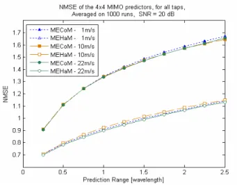
Fig. 4 shows the NMSE for both 4 x 4 predictors, initialized from 17 channel observations, with a SNR of 20 dB. There is still an obvious difference between the two predictors, but the user velocity does not have an influence.
Figure 4: NMSE for 4 x 4 MECoM and MEHaM, initialized from 17 observations, with SNR = 20 dB.
Means are obtained from 1,000 runs.
We will now end this section by summarizing our numerical results.
E. Summary of numerical computations
We have seen that the best choice for the number of observations is the smallest one. To explain this observation, one may conjecture that observations in excess do not bring any additional information to the model, but amplify noise. Moreover, using only a few observations has three main advantages. First the predictor does not require too much time to collect the observations it needs before being able to perform predictions (shorter warm-up time). Secondly, it limits the amount of information which has to be fed back to the transmitter. Finally, using a few observations reduces the size of all matrices we handle in the computations, which makes these computations faster and less greedy for computational power. Note that for a 4 x 4 MIMO channel, we need at least 17 observations to count more rows than columns in the H matrix described in (4). So 17 is a minimum, and waiting for 17 observations, with the parameters we used, corresponds to a warm-up period of 63.75 ms (127.5 TTIs).
We investigated the influence of the mobile user velocity on the accuracy of the predictions. From this velocity depends the maximum Doppler frequency and the coherence time. One would think the accuracy of the predictions is linked to the velocity, and the faster a user moves, the faster predictions would become poor. But our simulations showed that moving at 1 m/s or 20 times faster ends up with the same NMSE. We also have seen that the MEHaM scheme produces better results than the MECoM one, which is drawn from the original ESPRIT technique. Moreover, MEHaM is less sensitive to noise: the results with a SNR of 20 dB are barely the same as the one obtained with the unpractical SNR of 100 dB, and the results with 3dB are not so different. Remember that the MECoM scheme is adapted with respect to the channel variability, whereas MEHaM uses fixed values instead.
We will now end this paper with a list of conclusions and we will discuss a bit about future work items.
V. CONCLUSIONS
We presented two innovative wireless MIMO channel predictors, both based on SISO ESPRIT techniques. The MIMO channel is modeled for each transmit/receive antenna pair as a sum of weighted complex sinusoids. It means the channel is seen for each antenna pair as the sum of signal poles weighted by corresponding amplitudes. The poles depend on Doppler frequencies. Two techniques have been presented to find these poles: MECoM is based on [6], the original ESPRIT technique, using the time correlation matrix of the channel, and MEHaM is based on the idea of Andersen et al. presented in [5], where it only needs a Hankel matrix of the channel.
We have implemented these MIMO predictors in MATLAB scripts, and tested them using SCME [12] as a reference. It has been shown that 17 channel observations are needed to initialize the predictors in most of the cases. But for long term predictions (a few wavelengths away), using additional observations would be better. With our set-up, feeding the predictors with 17 observations implies to wait 63.75 ms before being able to predict the channel state. Moreover, the size of the matrices remains reasonable, so the computation is not too demanding. The effect of the noise is obviously to increase the NMSE of the predictors, but only for the first predicted values. After some time, the increase of noise improves the stability of the predictor. The variation of noise only has a limited effect on MEHaM: going down from a SNR of 20 dB to a SNR of 3 dB means an increase of the NMSE around 0.1 for the first predicted value. The MECoM predictor also has this behavior but variations are more important. The mobile user velocity does not have an influence on the results.
The MIMO predictors presented here are rather simple and do not require so many channel observations. Their performance are acceptable, but could be improved, for
instance by evaluating the impact of the Hankel matrix shape, i.e. the ratio (nT . nR .p) / q between its number of rows and
columns. The choice of the number of columns used with MEHaM, which is decided dynamically regarding the noise with MECoM, should also be further studied.
Moreover, all the numerical computations have been realized in the default MATLAB number resolution, which is 64 bits. We also considered a perfect CSI. A topic of interest for future work would be the investigation of the effects of a limited CSI feed back, quantized on only a few bits to limit the feedback throughput.
To consider practical use of the techniques, it would also be useful to work on refreshment schemes, performed at a fixed rate, or triggered when prediction errors become unacceptable.
REFERENCES
[1] S. Barbarossa, G. Scutari, S. Vergari, G. Paccapeli, “Robust Estimation and prediction methods for Time-Variant SISO channels”, IST ROMANTIK D421, June 2003
[2] S. Barbarossa, G. Paccapeli, G. Pecchini, G. Scutari, “Robust Estimation and prediction methods for Time-Variant MIMO Systems”, IST ROMANTIK D422, July 2003
[3] Z. Chen, J. Andrews and B. Evans, “Short Range Wireless Channel Prediction Using Local Information”, 37th Asilomar Conference on
Signals Systems Computers, Nov 2003.
[4] A. Arredondo, K. Dandekar and G. Xu, “Vector Channel Modeling and Prediction for the Improvement of Downlink Received Power”, IEEE
Transactions on Communication, Vol. 50, No. 7, July 2002.
[5] J.B. Andersen , J. Jensen, S.H. Jensen and F. Frederiksen, “ Prediction of Future Fading Based on Past Measurements”, IEEE Vehicular
Technology Conference – VTC’99- Spring, 1999.
[6] P. Stoica and R. Moses, Spectral Analysis of Signals, Pearson Prentice Hall, 2005.
[7] T. Ekman, Prediction of Mobile Radio Channels. Modelling and Design. PhD Th., Signals and Syst., Uppsala Univ, 2002. http://www.signal.uu.se/Publications/abstracts/a023.html
[8] T. Ekman, M. Sternad, and A. Ahlén, “Unbiaised Power Prediction of Rayleigh Fading Channels”, IEEE Vehicular Technology Conference
VTC’01-Spring, Rhodes, Greece, May 6-9 2001.
[9] M. Sternad, T. Ekman and A. Ahlén, “Power prediction on broadband channels”, IEEE Vehicular Technology Conference VTC’02-Fall, Vancouver, Canada, September 2002.
[10] M. Sternad and D. Aronsson, “Channel estimation and prediction for adaptive OFDM downlinks," IEEE Vehicular Technology Conference
VTC 2003-Fall, Orlando, Fla, Oct. 2003.
[11] M. Sternad and D. Aronsson, ”Channel estimation and prediction for adaptive OFDMA/TDMA uplinks, based on overlapping pilots”,
International Conference on Acoustics, Speech and Signal Processing (ICASSP 2005). Philadelphia, PA, USA, March 19-23 2005. Online:
http://www.signal.uu.se/Publications/abstracts/c0501.html
[12] 6th Framework Programme, Information Society Technologies, Wireless World Initiative New Radio (WINNER), IST-2003-507591, [online] Available: https://www.ist-winner.org/
[13] M. Guillaud and D. Slock in “Pathwise MIMO Channel Modelling and Estimation”, IEEE International Workshop on Signal Processing
Advances for Wireless Communications (SPAWC 05). New York, NY,
USA, June 5-8 2005
[14] "Physical layer aspects for evolved Universal Terrestrial Radio Access (UTRA)", 3GPP TR 25.814 v7.1.0, September 2006