A simple correction method of inner filter effects affecting FEEM and its application to the PARAFAC decomposition

HAL Id: hal-00807769

https://hal.archives-ouvertes.fr/hal-00807769

HAL is a multi-disciplinary open access

archive for the deposit and dissemination of sci-entific research documents, whether they are pub-lished or not. The documents may come from teaching and research institutions in France or abroad, or from public or private research centers.

L’archive ouverte pluridisciplinaire HAL, est destinée au dépôt et à la diffusion de documents scientifiques de niveau recherche, publiés ou non, émanant des établissements d’enseignement et de recherche français ou étrangers, des laboratoires publics ou privés.

A simple correction method of inner filter effects

affecting FEEM and its application to the PARAFAC

decomposition

Xavier Luciani, Stéphane Mounier, Roland Redon, André Bois

To cite this version:

Xavier Luciani, Stéphane Mounier, Roland Redon, André Bois. A simple correction method of inner filter effects affecting FEEM and its application to the PARAFAC decomposition. Chemometrics and Intelligent Laboratory Systems, Elsevier, 2009, 96 (2), pp.227-238. �10.1016/j.chemolab.2009.02.008�. �hal-00807769�

A simple correction method of inner filter

effects affecting FEEM and its application to

the PARAFAC decomposition

X. Luciani

∗, S. Mounier

, R. Redon

, A. Bois

06903 Sophia Antipolis Cedex - France

b_{Laboratoire PROTEE, USTV, BP 20132, 83957 La Garde Cedex, France}

Abstract

In this paper we introduce a new inner filters correction method for standard flu-orometer. The Controlled Dilution Approach (CDA) deals with highly absorbing solutions using the Fluorescent Excitation-Emission Matrix of a controlled weak dilution. Along with the non linear FEEM of the original solution, these two infor-mations allow to estimate the linearized FEEM. The method relies on inner filter effects modelization. Beyond its numerical simplicity, the main interest is that CDA only requires fluorescence measurements. The method was validated using a set of known mixtures and a set of dissolved organic matter samples. In addition we show that the corrected FEEM can be used efficiently for advanced multilinear analy-sis. Therefore CDA is presented here as a relevant pretreatment to the PARAFAC decomposition of highly absorbing mixtures.

Key words: EEM, inner filter effects, PARAFAC, 3D fluorescence

∗ Corresponding autor.

1 Introduction

1

1.1 Non linearities in fluorescence spectroscopy

2

Fluorescent molecular components (fluorophores) can be easily distinguished

3

by their spectroscopic properties and more particularly by their fluorescence

4

spectra [1]. Recent fluorometers provide successive measurements of the

flu-5

orescence intensity emitted by a solution of one or several fluorophores. By

6

scanning excitation and emission wavelength domains, Fluorescent

Excitation-7

Emission Matrices (FEEM) gather a lot of informations about the solution.

8

These spectra are now widely used in various scientific domains such as medicine

9

[2], analytical chemistry [3] or environmental sciences [4,5].

10

Ideally, considering the FEEM (I3D) of a single fluorophore, its norm is

pro-11

portional to the fluorophore concentration in the solution and its pattern is

12

given by the outer product between the excitation spectrum and the emission

13

spectrum of the fluorophore. This is the classical linear model of fluorescence.

14

However it is well known that its pertinence decreases with the concentration

15

[6]. Actually, non linear deviations mean that the gradual absorption by the

16

solution of both exciting and fluorescent lights cannot be neglected. These

17

effects are known as inner filter effects and affect both I3D norm and I3D

18

pattern. Therefore, in presence of inner filter effects, one cannot deduce any

19

correct information about the solution directly from I3D.

20 21 Emission (nm) 3.54 ppm Excitation (nm) 300 350 400 350 400 450 500 550 600 51.54 ppm 300 350 400 350 400 450 500 550 600 108.75 ppm 300 350 400 350 400 450 500 550 600 0 0.5 1 1.5 2 2.5 3 3.5 4 x 10−3

Fig. 1. Evolution of the quinine sulphate 3D spectrum for three different concentra-tions: 3.54 ppm (left spectrum), 51.54 ppm (middle spectrum), 108.75 ppm (right spectrum)

Example of inner filter effects is given on figure 1. This example clearly shows

22

that the FEEM pattern can be severely affected even in the simple case of a

23

single fluorophore solution.

24

In other respects, considering several solutions of the same diluted fluorophore

measured in different conditions, many other factors such as diffusion,

tem-26

perature variations, pH variations, fluorescence quenching or ionic strength

27

can affect the FEEM linearity [1]. In this work, we only focus on inner filter

28

effects correction.

29

30

1.2 Inner filter effects correction

31

Inner filter effects are observed and studied for a long time now [7,8]. Two

32

main correction methods are used to prevent these deviations. Since inner

33

filter effects can be neglected for weak absorbances i.e. weak concentrations, a

34

common procedure is to strongly dilute the solution until maximal absorbance

35

is inferior than 0.1 [1]. There is an obvious drawback with this dilution method

36

as a too strong diluting factor would severely reduce the signal to noise ratio.

37

Moreover this procedure must be applied very carefully to avoid contamination

38

or physico-chemical changes. Therefore, ensuring the linearity of the data set

39

is no easy task. The second approach uses a mathematical model of inner filter

40

effects [9–11]. Then one can deduce a correction factor in order to estimate

41

element by element, a corrected FEEM (Ic) from I3D. It is assumed that if the

42

correction factor is suitable then Ic will follow the linear model. This approach

43

relies on the Beer-Lambert law [1] which gives the elementary variation dI of

44

the light intensity through an elementary optical path dl at wavelength λ:

45

dI = −I(λ)α(λ)dl (1)

where α is the absorption coefficient of the solution. Then, the integrated

46

law describes the light absorption through the entire optical path. If I0 is the

47

intensity of the exciting light, the transmitted intensity outside a cell of length

48

l is simply given by the relation:

49

I(λ) = I0(λ)e−α(λ)l = I0(λ)10−A(λ) (2)

The absorbance spectrum of the solution is then defined by

50 A(λ) = log10 I0(λ) I(λ) ! = lα log(10) (3)

Figure 2 shows a schematic diagram of absorbance measurement. A is obtained

51

by measuring the transmitted intensity through the diluted solution (IT) and

52

the transmitted intensity through the solvent (IR) at successive wavelength:

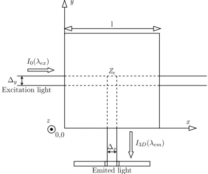
53 A(λ) = log10 IR(λ) IT(λ) ! (4) In right angle fluorescence spectroscopy, classical model of inner filter effects

54

is given by equation 5.

Monochromator

Source Semitransparent mirror

Mirror Mirror I0 I0 IT IR Detector Detector Solution Solvent

Fig. 2. Absorbance measurement

I3D(λex, λem) = Ic10−

A(λex)+A(λem)

2 (5)

Thereby, one can use the measured absorbance spectrum to compute the

cor-56

rection factor and then deduce Ic. Similar methods were proposed in [12–14].

57

In the following, this approach will be identified as the Absorbance Correction

58

Approach (ACA). ACA is commonly used in applicative papers dealing with

59

fluorescence spectroscopy [15,16]. However absorbance measurement is much

60

less sensitive than fluorescence measurement. In addition it requires an other

61

experimental device whose characteristics are different, introducing its own

62

error in the chain. Finally, the short linear range of absorption measurement

63

is another important drawback of ACA. In this work we propose an original

64

correction method: the Controlled Dilution Approach (CDA) which combines

65

the advantages of both methods. CDA uses the FEEM of a diluted solution

66

instead of absorbance measurement in order to estimate Ic. The crucial point

67

is that the dilution factor can be chosen small enough to avoid the drawback

68

of the dilution approach. Indeed, the linearity of this second FEEM is not

re-69

quired. Consequently, CDA keeps the main advantage of ACA which is a very

70

simple numerical correction, but it only requires fluorescence spectra.

Anal-71

ized solutions are generally mixtures of several fluorophores. Therefore, many

72

applications involve a separation step to recover the underlying individual

73

spectra and concentration profiles of each fluorophore. Number of

chemomet-74

ric methods were proposed in the literature in order to perform multilinear

75

decompositions of FEEM [17–20]. Based on original works of Harshman [21],

76

PARAllel FACtor analysis (PARAFAC) was introduced in this context by Bro

77

[22]. During the last decade PARAFAC has proved to be the most relevant

78

approach. For instance, in environmental sciences, it is currently the reference

79

tool to characterize and trace Dissolved Organic Matter (DOM) [23–25]. In

80

return, it do not take into account inner filter effects [26,27]. Consequently

81

there is an irreversible loss of performance when dealing with highly

absorb-82

ing mixtures.

Like other inner filter effects correction methods, CDA is independent of this

84

separation step. However, we take into consideration that a large part of FEEM

85

applications, uses this kind of decomposition. As a consequence, in order to

86

ensure the reliability of CDA, we also present in this paper its performance as

87

a PARAFAC pretreatment of highly absorbing mixtures.

88

89

1.3 Paper organization

90

CDA is detailed on section 2 of this paper. First the modelization of inner

91

filter effects is given in section 2.1 then CDA is described on section 2.2.

92

Lastly, practical aspects of CDA are presented in section 2.3 notably in the

93

case of FEEM sets analysis. The PARAFAC application to the CDA corrected

94

FEEM is shortly describe.

95

In this work, CDA correction is experimentally tested on two very different

96

sets of mixtures. The first set is composed of standard laboratory mixtures

97

of fluorescein and quinine sulphate. Consequently, thist first data set is used

98

to strictly validate CDA and compare with classical ACA. On the other side,

99

the second data set is constituted by unknown samples of DOM catchments

100

and gives an example of how the method can help in a realistic case. Section

101

3 describes the experimental part of these tests. Results obtained on both

102

data sets before and after the PARAFAC decomposition are presented and

103

discussed in section 4.

104

2 Theory

105

2.1 Modelization of inner filter effects

106

Like ACA, CDA relies on equation 5. Few authors give detailed mathematical

107

justifications of this model, particularly in the most general case of 3D spectra

108

of fluorophore mixtures. In this subsection a rigorous interpretation of

equa-109

tion 5 is proposed.

110

We consider here a mixture of N fluorophores. For each fluorophore n, we

111

note cn its concentration in the solution, εn(λex) its molar extinction

coeffi-112

cient at the excitation wavelength λex, Φn its the quantum yield of fluorophore

113

n, γn(λem) its emission probability at wavelength λem and αn(λex) its

absorp-114

tion coefficient which is equal to the product of cn by εn(λex). We assume

115

that the absorption and emission spectra of fluorophore n are normalized

val-116

ues of respectively εn(λex) and γn(λem). In the linear approximation, every

117

fluorescing particles are treated equally as if the whole sample cell was an

mentary point. In order to improve this model, one should takes into account

119

the particular geometry of the problem.

120 I3D I0 Ex itationdevi e Emissiondevi e Sample ell x y z

Fig. 3. Schematic diagram of right angle fluorescence measurement

Figure 3 recalls basically the experimental device of right angle standard

flu-121

orometers. The excitation light (I0(λex)) is absorbed through the sample cell

122

(length l) by the fluororphores, inducing the fluorescent light. Finally, a

frac-123

tion (I3D(λem)) of the emitted signal is collected perpendicularly to the

excit-124

ing beam. λex and λem scannings allow to measure the FEEM.

125

In this study, several approximations were made. First of all, we took into

126

consideration the symmetry of the problem, therefore the influence of the z

127

spatial dimension was neglected.

128 I₀(λex) I_3D(λem) Ze ∆y ∆x Emitedlight l 0,0 y x Ex itationlight z

Secondly, only two main optical paths were considered. They represent the

129

excitation beam and emission beam in figure 4 scheme. This means that the

130

fraction of the exciting light which do not reach the ”influence zone” Ze was

131

neglected as well as the fluorescence light issued from the region outside Ze.

132

Then each elementary segment of the ”excited face” of Ze was supposed to

133

receive the same energy from the rectilinear exciting beam. In the same way,

134

we assumed that each elementary segment of the ”emission face” of Zeprovides

135

the same energy to the detector. Furthermore, diffusion and re-emission effects

136

were also neglected. Actually we only consider the elementary optical paths

137 represented in figure 5. 138 Ze

∆

∆

Fig. 5. Elementary cutting of the ”influence zone” in the directions of exciting and emitted ligthts

The integrated Beer-Lambert law describes the light absorption through the

139

optical path. If I0 is the light intensity at the point x0 of the dilute solution,

140

the intensity in x is simply given by the relation: I = I0e−α(λex)(x−x0) where α

141

is the mixture total absorption coefficient: α =P

nαn. The influence zone was

142

divided into horizontal and vertical elementary strips of respective dimension

143

dy× l and l × dx. Then each horizontal strip receives an equal elementary

144

fraction of the exciting light: dyI0

∆y and the Beer-Lambert law quantifies the 145

intensity transmitted to x. A fraction αndx is absorbed by fluorophore n, and

146

the total intensity absorbed by fluorophore n in the ”influence zone” (IAn) is

147 given by: 148 IAn(λex) = dyI0 ∆y αn(λex) Z l+∆x₂ l−∆x 2 e−α(λex)x_{dx (6)}

IAn(λex) = 2 I0 ∆yα(λex) αn(λex)e− α(λex)l 2 sinh α(λex)∆x 2 ! dy (7)

The fluorescence signal emitted by the dy strip at wavelength λem is equal

149

toP

nΦnγn(λem)IAn(λex) and the Beer-Lambert law integrated on all the

ele-150

mentary horizontal strips gives the ratio of the fluorescence signal transmitted

151

outside the sample cell in the y direction, I3D(λex, λem).

152 I3D(λex, λem) = Z l+∆y₂ l−∆y 2 X n Φnγn(λem)IAn(λex)e−α(λem)y (8) I3D(λex, λem) = 4I0e− α(λex)l 2 sinh(α(λex)∆x 2 )e− α(λem)l 2 sinh(α(λem)∆y 2 ) ∆yα(λex)α(λem) X n αn(λex)Φnγn(λem) (9) α(λex)∆x 2 and α(λem)∆y

2 are supposed to be small enough to make the following

153 approximation: 154 I3D(λex, λem) = I0∆x X n αn(λex)Φnγn(λem) ! e−α(λex)l_{2 e}−α(λem)l_{2 (10)}

Then we can define g = l

2 and Gn= I0∆xΦn. This leads to the final expression

155 of the model: 156 I3D(λex, λem) = N X n=1 Gncnεn(λex)γn(λem) ! _N Y n=1 e−g(cnεn(λex)+cnεn(λem)) ₍₁₁₎

In the following we define

157 L(λex, λem) = N X n=1 Gncnεn(λex)γn(λem) (12) then we have 158 I3D(λex, λem) = Le−g(cnεn(λex)+cnεn(λem)) (13) This equation is clearly equivalent to equation 5 with Ic = L. Its first order

159

approximation is justified for small enough concentrations. In this case, since

160

the exponential term tends to 1 one obtains the linear model of fluorescence.

161

Correction of inner filter effects simplifies spectral analysis. It is interesting

162

to note that their modelization is also used in another context. Actually, a

163

recent article [28] highlighted the major contribution of inner filter effects in

164

the phenomenon of concentration-dependent red-shift [29,30]. In this work, a

165

similar model has been successfully used to optimize synchronous fluorescence

166

spectroscopy of concentrated mixtures of fluorophores.

2.2 Controlled Dilution Approach

168

The previous model describes non linear effects but the related equation can

169

still be considered as a bilinear decomposition involving some modified

indi-170 vidual spectra ε′ n(λex) and γn′(λem) : 171 I3D(λex, λem) = N X n=1 ε′ n(λex)γn′(λem) (14) with, 172 ε′ n(λex) = Gncnεn(λex)e− PN p=1gcpεp(λex) (15) γ′ n(λem) = γn(λem)e− PN p=1gcpεp(λem) ₍₁₆₎

It is well known that bilinear decompositions have an infinite number of

equiv-173

alent solutions in the least square sense. Therefore, without additional

infor-174

mation, no mathematical tool can diagnose whether a FEEM is affected by

175

inner filter effects or not. A fortiori additional informations are also needed to

176

correct inner filter effects. In ACA this information is the solution absorbance

177

spectrum. This section shows how the correction can be made with fluorescent

178

spectra only.

179

According to equation 11 the FEEM I3D of a N fluorophores mixture is the

180

product of a linear (L) term in respect of concentrations and spectra by a non

181

linear one, denoted H:

182 H(λex, λem) = N Y n=1 exp(−g(cnεn(λex) + cnεn(λem)) (17) So we can write: 183 I3D(λex, λem) = L(λex, λem)H(λex, λem) (18) Now, let’s I3Dp be the FEEM of the same mixture, diluted by a factor p, then 184 we have: 185 I3Dp(λex, λem) = N X n=1 Gn cn pεn(λex)γn(λem) ! _N Y n=1 e−g(cnpεn(λex)+cnpεn(λem)) (19) I3Dp(λex, λem) = 1 pL(λex, λem)H 1 p(λ ex, λem) (20)

The analytical resolution of 18 and 20 gives

186 L(λex, λem) = (pI3Dp(λex, λem)) p I3D(λex, λem) ! 1 p−1 (21) H(λex, λem) = I3D(λex, λem) pI3Dp(λex, λem) ! p p−1 (22)

The L term is the corrected FEEM estimated by CDA, corresponding to the linear model of fluorescence. As previously mentioned, the correction only re-quires the original FEEM and the diluted FEEM and the value of the dilution factor p.

The sensitivity of the estimator of L to p is difficult to quantify. A first order approximation of the variability of L (∆L) leads to:

∆L

L =

(p − 1 − log(p) − log(I3Dp) + log(I3D))∆p (p − 1)2

According to this equation, a high factor should be preferred. However it would

187

involve the drawbacks of a strong dilution (see section 1.2). Finally, we

advo-188

cate for a dilution factor corresponding to the simplest dilution process, thus

189

the experimental uncertainty ∆p is minimized. This was the case for all the

190

experiments presented in this study.

191

Owing to the term by term division in equation 21, noisy values in the

mea-192

sured FEEM could affect the estimation of L. Actually if the division involves

193

two small values relatively to the noise level, some very narrow and localized

194

peaks can appear. Fluorescent spectroscopy is a very sensitive technique

there-195

fore this kind of deviation are rarely observed in practical situations. Otherwise

196

those peaks appear outside the main fluorescing areas. In consequence, they

197

can be easily detected and filtered without damaging the fluorescent peaks.

198

199

2.3 CDA and multilinear analysis of concentrated fluorescing mixtures

200

We consider now a set of I mixtures and cn(i) denotes the concentration of

201

fluorophore n in mixture i. CDA methodology is simple, the correction is done

202

sample by sample. The first step consists in choosing the dilution factor p for

203

each sample (see the end of section 2.2). Obviously the same value can be used

204

for every sample. Then, the corresponding controlled dilution is performed

205

and both FEEM I3D and I3Dp are measured. Before correction, Rayleigh and

206

Raman scatters must be corrected carefully on each FEEM. This is the end

207

of the experimental and pre-processing steps.

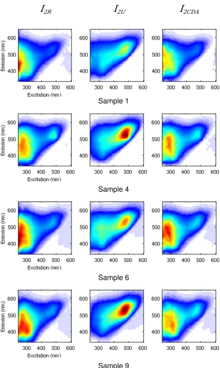
208

Finally, for each sample i, the estimation L(i, λex, λem) of the linearized FEEM

209

is obtained directly from equation 21. At this stage, the correction of the inner

210

filter effects is completed.

211

Actually we have to take into account measurement and modelization errors.

212

In addition we can define ˜cn(i) = Gncn(i). Therefore in practice, definition 12

213 is rewritten: 214 L(i, λex, λem) = N X n=1 ˜ cn(i)εn(λex)γn(λem) + E(i, λex, λem) (23)

where E is the error term. Equation 23 is a rank N decomposition of the 3

215

way tensor L or in other words a 3-way PARAFAC model of rank N. For

216

each fluorophore n, the loading vectors of the decomposition ˜cn, εn, and γn

217

are linearly linked to its concentration profile, its excitation spectrum and its

218

emission spectrum respectively. Moreover, the solution of this decomposition

219

is unique up to trivial scaling and position indeterminacy [31,32]. Finally,

sev-220

eral efficient algorithms were proposed and compared for the estimation of the

221

loading vectors. These are largely described in the literature [33–35]. Those

222

three physical, mathematical and practical reasons made the PARAFAC

de-223

composition the most suitable tool for analysing linear(ized) FEEM. Tutorials

224

and examples of PARAFAC application to FEEM analysis can be found

else-225

where [36,22,37].

226

Eventually, the PARAFAC decomposition can be run normally on the

cor-227

rected FEEM set in order to find out real individual spectra and concentration

228

profiles of each fluorophore.

229

230

3 Experimental

231

3.1 Data set 1, standard mixtures

232

Seven solutions (Si

1, i = 1 · · · 7) with different concentrations of fluorescein

233

(Aldrich) and quinine sulphate (Merkc) were prepared in 0.1M H2SO4(Aldrich)

234

in order to validate the correction method. All chemicals are analytical grade.

235

Concentrations in fluorescein and quinine sulphate are given in table 1 along

236

with solution absorbances. These two fluorophores and their concentrations in

237

the solutions were chosen because of their good fluorescing ability and their

238

overlapped spectra in order to emphasize inner filter effects.

239

Table 1

Concentrations, maximal absorbances and mean absorbances of the original solu-tions of quinine sulphate and fluorescein.

Solution S1 1 S21 S31 S14 S51 S61 S71 cSQ (ppm) 0 11.02 32.6 54.38 76.15 97.73 108.75 cF (ppm) 83.15 74.72 58.23 41.58 24.92 8.43 0 Absorbance max. 2.30 2.18 1.83 1.32 1.17 1.38 1.47 Mean Absorbance. 0.42 0.40 0.37 0.33 0.29 0.27 0.24

Concentrations in quinine sulphate (cSQ) and fluorescein (cF) are given in parts per

million (ppm). Maximum and mean value of absorbance are relative to the 275 to 500 nm excitation range.

Seven twice diluted solutions (Si

1D, i= 1 · · · 7) were obtained by mixing equal

240

volumes of initial solutions Si

1 and 0.1M of H2SO4. Table 2 gives the actual

241

value of the dilution factor for the seven solutions and the standard deviation

242

due to the pipet precision.

243

Table 2

Dilution factors used for the seven solutions of fluorescein and quinine sulphate. Solution S1_1D S2_1D S3_1D S4_1D S5_1D S6_1D S7_1D

p 2.11 2.08 2.07 2.07 2.07 2.08 2.11 σp 0.034 0.032 0.030 0.029 0.030 0.032 0.034

σp is the estimated standard deviation of the dilution factor due to the experimental

dilution

Reference solutions (Si

1R, i = 1 · · · 7) were obtained by diluting 100 µL of S1i

244

in 3000 µL of 0.1M of H2SO4. In this case of simple mixtures, this dilution

245

prevents inner filter effects without physico-chemical changes.

246

All measured spectra were obtained with a fluorometer Hitachi F4500. FEEM

247

of the three solutions sets S1, S1D and S1R, were recorded at 30000 nm/min

248

scan speed from 350 to 700 nm in emission by step of 5 nm and for excitation

249

wavelength from 275 to 500 nm by step of 5 nm. Excitation and emission

band-250

width were 5 nm. Fluorescence intensity was corrected from PM response using

251

manufacturer setting. Data for FEEM treatment were extracted by FLWinLab

252

software for emission and excitation range stepped every 5 nm. Rayleigh and

253

Raman scatters were removed numerically by the method proposed by Zepp

254

in [38]. In the following, measured FEEM from original, diluted and reference

255

solution i will be referred as Ii

1U, I1Di and I1Ri respectively. Absorption

spec-256

tra of solutions S1 were obtained from transmittance spectra recorded with

257

absorbance mode of the F4500 (speedscan 240 nm/min) from 200 to 800 nm

258

with 5 nm bandwidths in excitation and emission. 2D reference spectra of

flu-259

orescein and quinine sulphate were recorded from S1

1R and S1R7 respectively, at

260

240 nm/min scan speed by step of 1 nm with 5 nm bandwidth in excitation

261

and 2.5 nm bandwidth in emission. Quinine sulphate (I_SQ−ex) and fluorescein

262

(IF −ex) excitation spectra were recorded from 275 to 500 nm at 450 nm and

263

510 nm emission wavelength respectively. Their emission spectra (ISQ−emand

264

I_{F −em}) were recorded from 350 to 700 nm at 340 nm and 440 nm excitation

265

wavelength respectively.

266

I1R and I1U compose the groups of reference and uncorrected FEEM

respec-267

tively. Using absorption spectra in equation 5, we could compute the ACA

268

corrected FEEM (Ii

1ACA) from I1Ui , i = 1 · · · 7. In the same way, using I1Di in

269

equation 21 with dilution factor values of table 2, we could apply CDA to Ii 1U

270

and compute the CDA corrected FEEM (Ii

1CDA), i = 1 · · · 7. I1ACA and I1CDA

271

compose the groups of ACA and CDA corrected FEEM respectively.

272

These four groups of FEEM are considered as four 3-way tensors of dimensions

273

7 × 46 × 51. Trilinear decompositions of these tensors were performed with the

274

PARAFAC-ALS algorithm of the nway toolbox for Matlab [39].

3.2 Data set 2, unknown samples

276

The second data set is composed of FEEM obtained from eleven samples

277

of concentrated humic acid solutions which were extracted from catchments

278

of Cameron soils. For each sample, 1 g of soil was extracted by 30 mL of

279

HCl(1M) solution. After separation, the supernatant solution was cleaned on

280

XAD-8 resin and stored at 4◦_{C in dark. The resting soil was then extracted}

281

with 30 mL of 1M NaOH solution. After separation, this second supernatant

282

contains humic acid substance. Purification was done by acidic precipitation

283

and sodic redissolution. Humic acid gave dark brown solution and fulvic acid

284

yellow solution. Original solutions (Si

2, i = 1 · · · 11), were obtained by

dilut-285

ing 100 µL of the extracted solutions in 3000 µL of 0.1M NaOH buffer. All

286

chemicals are analytical grade. Eleven twice diluted solutions in 0.1M NaOH

287

buffer (Si

2D, i= 1 · · · 11) were also prepared. Finally, reference solutions

with-288

out inner filter effect (Si

2R, i= 1 · · · 11) were obtained by 15 times dilutions of

289

S_2Di .

290

FEEM of Si

2 (I2Ui ), S2Di (I2Di ) and S2Ri (I2Ri ) were recorded for i = 1 · · · 11, at

291

30000 nm/min scan speed from 340 to 650 nm in emission for excitation

wave-292

length from 240 to 600 nm, by emission and excitation step of 5 nm and with

293

10 nm bandwidth in excitation and 5 nm bandwidth in emission. Rayleigh

294

and Raman scatters were consistently corrected [38].

295

I2R and I2U compose the groups of reference and uncorrected FEEM

respec-296

tively. Using Ii

2D in equation 21 with p = 2, we could apply CDA to I2Ui and

297

compute the CDA corrected FEEM (Ii

2CDA), i = 1 · · · 11. I2CDA compose the

298

group of CDA corrected FEEM. Comparison with ACA was not made on this

299

data set.

300

Hence, three tensors of dimensions 11×73×63 were obtained and decomposed

301

by PARAFAC-ALS [39].

302

4 Results and discussion

303

In the following the PARAFAC applications to uncorrected, reference, ACA

304

corrected and CDA corrected groups of FEEM will be referred as U-PARAFAC,

305

R-PARAFAC, ACA-PARAFAC and CDA-PARAFAC respectively.

306

4.1 Data set 1

307

Each CDA corrected FEEM (Ii

1CDA, i = 1 · · · 7) are firstly compared to I1Ri ,

308

Ii

1U and I1ACAi . Representative examples of these FEEM are presented on figure

309

6 for i = {1, 3, 4, 6}. In these examples, CDA provides satisfying estimations

of the reference FEEM in spite of a small distortion in the fluorescein peak

311

(440/510nm), particularly on I1

1CDA . In order to quantify these comparisons

312

three relative squared residual error terms (ri

1CDA, r1Ui and r1ACAi ) were

com-313

puted as follow for each solution i and stored in table 3.

314 ri_1CDA= P j,k(I1Ri (j, k) − I1CDAi (j, k))2 P i,jI1Ri (j, k)2 (24) r_1Ui = P j,k(I1Ri (j, k) − I1Ui (j, k))2 P j,kI1Ri (j, k)2 (25) r_1ACAi = P j,k(I1Ri (j, k) − I1ACAi (j, k))2 P j,kI1Ri (j, k)2 (26) The significance of the non linear term in equation (11) increases with the

Table 3

Comparison of the relative squared residual error terms(in % ) for the seven solution of data set 1. Solution 1 2 3 4 5 6 7 r1U 117 109 81 46 29 20 13 r1ACA 31 38 59 33 14 7 8 r1CDA 11 5 2 1.8 0.3 0.06 0.03 315

solution absorbance. Therefore comparing tables 1 and 3, there is an obvious

316

correlation between r1U and the mean absorbances as both values decrease

317

regularly from solutions 1 to 7. The same observation holds true regarding

318

r1CDA. The correlation is less apparent for r1ACA but globally the error is

319

greater for solutions 1 to 4 than for the least absorbing solutions. r1U values

320

are comprised between 13% and 117%. After CDA correction, these boundary

321

values decreased to 0.03% and 11% respectively . These results are very

sat-322

isfying for solutions 2 to 7. The first solution shows a stronger error but there

323

is still a clear improvement in comparison of the original FEEM. CDA results

324

are always clearly better than ACA ones. Actually, in the more favourable

325

case in respect to ACA results (solution 1), r1ACA is almost 3 times greater

326

than r1CDA.

327

These results showed that CDA provided a better estimation of I1R than

328

ACA. In order to verify if CDA correction is satisfying for further analysis,

329

the PARAFAC-ALS algorithm was applied to the four groups of FEEM. For

330

each group, the core consistency diagnostic (CORCONDIA) [40] suggested

331

two as the right number of components. Consequently, each PARAFAC

de-332

composition provides an estimation of the quinine sulphate and fluorescein

333

excitation and emission spectra and an estimation of their relative

concen-334

trations trough the data set. After normalisation, the relative squared error

335

(rc_{, r}ex _{and r}em_{) between the PARAFAC loadings and the real variables are}

336

compared on tables 4 to 6. In the case of the spectral loadings, two other

spec-337

troscopic criteria are also used: the relative error to the maximum value of the

Fig. 6. Illustrations of I1R, I1U, I1ACA and I1CDAfor solutions 1, 3, 4 and 6 of data

set 1.

spectrum and the shift on the position of the maximum. In addition,

load-339

ings obtained from U-PARAFAC and CDA-PARAFAC are shown on figures

340

7 to 9, along with real spectra and profiles. A first global remark should be

341

made: the perfect agreement on the three modes between the real variables and

342

R-PARAFAC loadings demonstrates that estimation errors of U-PARAFAC,

ACA-PARAFAC and CDA-PARAFAC are mainly due to inner filter effects

344

and not to the PARAFAC decomposition.

345

346

Table 4

Data set 1, concentration mode results. Relative squared residual error in percent between the real profiles and their estimation from I1R (r_1Rc ), I1U (rc_1U), I1ACA

(rc

1ACA) and I1CDA (rc1CDA).

Fluorophore rc_1R r_1Uc r_1ACAc rc_1CDA Quinine sulphate 0.1 8.3 0.7 0.2 Fluorescein 0.08 23 0.4 4.2 0 1 2 3 4 5 6 7 88 0 0.1 0.2 0.3 0.4 0.5 0.6 0.7 0.8 0.8 Solution number relative concentrations Quinine Sulphate 0 1 2 3 4 5 6 7 8 0 0.1 0.2 0.3 0.4 0.5 0.6 0.7 Fluorescein

Fig. 7. Data set 1, PARAFAC loadings of the concentration mode: Real spectra (solid ∗ line), U-PARAFAC loadings (dot ⋄ line) and CDA-PARAFAC loadings (dash △ line)

Results for the concentration mode are presented in table 4 and figure 7.

347

The shape of the concentration profile of the quinine sulphate is slightly

af-348

fected by filter effects (rc

1U = 8.3%). However CDA-PARAFAC gives much

349

more accurate results for each solution (rc

1CDA = 0.2%). ACA-PARAFAC is

350

also satisfying but it is not as efficient as CDA. The concentration profile of

351

the fluorescein is more distorted (rc

1U = 23%). CDA-PARAFAC performs well

352

(rc

1CDA = 4.2%) but the relative error is still high for the first solution. It

353

should be noted that ACA-PARAFAC (rc

1ACA = 0.4%) do better than

CDA-354

PARAFAC. This last result is surprising because it is in contradiction with

355

the five other loadings.

356

357

Results for the excitation mode are presented in table 5 and figure 8. The

358

excitation mode is the most affected by inner filter effects, with rex

1U values of

359

12.9% and 95.15% for quinine sulphate and fluorescein respectively.

Consid-360

ering figure 8, quinine sulphate excitation spectrum is widened and flattened

361

by inner filter effects. These distortions are completely eliminated by

Table 5

Data set 1, excitation mode results. Comparison with the real spectra among three criteria: relative error on the maximum value (%), shift (nm) and relative squared error (%)

Fluorophore Criterion Ref. Unc. ACA cor. CDA cor.

Rel. err. max. val. 0.4 24 23 0.5

Quinine sulphate Shift. 0 20 0 0

rex 0.06 12.9 4.1 0.08

Rel. err. max. val. 2.5 50.5 15 17

Fluorescein Shift 0 20 5 5 rex 0.07 95.15 9.3 3.4 200 300 400 500 0 0.1 0.2 0.3 0.4 Quinine Sulphate Intensity (a.u.) Excitation (nm) 300 400 500 0 0.1 0.2 0.3 0.4 0.5 Fluorescein

Fig. 8. Data set 1, PARAFAC loadings of the excitation mode: Real spectra (solid line), U-PARAFAC loadings (dot line) and CDA-PARAFAC loadings (dash line)

PARAFAC. Indeed, the CDA-PARAFAC estimated spectrum is really close

363

to the real spectrum (rex

1CDA = 0.08%). ACA-PARAFAC (r1ACAex = 4.1%)

glob-364

ally improves U-PARAFAC result (rex

1U = 12.9%). The relative error on the

365

maximum value is negligible with CDA-PARAFAC (0.5%) while it as

impor-366

tant with ACA-PARAFAC (23%) as without correction (24%). The 20 nm

367

shift on the position of the maximum is perfectly corrected by both

CDA-368

PARAFAC and ACA-PARAFAC. These observations hold true for the

fluo-369

rescein spectrum but the gaps between the different estimations are wider.

370

The spectrum estimated by U-PARAFAC is totally distorted in respect to the

371

real spectrum, rex

1U = 95.15%. In spite of some residual distortions

(flatten-372

ing and widening), the spectrum shape is almost fully recovered with CDA

373

correction (rex

1CDA= 3.4%). ACA-PARAFAC global estimation is not as good

374

(rex

1ACA = 9.3%). In absence of correction, the relative error on the maximum

375

value is very high (50.5%). ACA-PARAFAC and CDA-PARAFAC relative

376

error are equivalent with 15% and 17% respectively. In the same way the

maximum shift is limited by ACA-PARAFAC and CDA-PARAFAC to the

378

fluorometer excitation step (5 nm) against 20 nm with U-PARAFAC.

379

Table 6

Data set 1, emission mode results. Comparison with the real spectra among three criteria: relative error on the maximum value (%), shift (nm) and relative squared error (%)

Fluorophore Criterion Ref. Unc. ACA cor. CDA cor. Rel. err. max. val. 1.4 4.1 4.1 0.7

Quinine sulphate Shift 0 5 5 0

rem 0.06 1.8 0.17 0.1

Rel. err. max. val. 3.9 4 4.7 0.6

Fluorescein Shift 0 0 15 0 rem 0.4 7.6 15 0.5 400 500 600 700 0 0.1 0.2 0.3 0.4 Emission (nm) Intensity (a.u.) Quinine Sulphate 400 500 600 700 0 0.1 0.2 0.3 0.4 Fluorescein

Fig. 9. Data set 1, PARAFAC loadings of the emission mode: Real spectra (solid line), U-PARAFAC loadings (dot line) and CDA-PARAFAC loadings (dash line)

Results for emission mode are presented in table 6 and figure 9. The

emis-380

sion spectrum of quinine sulphate is well estimated by U-PARAFAC (rem

1U =

381

1.8%). However ACA-PARAFAC and CDA-PARAFAC still improve this

re-382

sult in different proportions (rem

1ACA = 0.17% and r1CDAem = 0.1%). One should

383

note that the relative error on the maximum value is the same with

ACA-384

PARAFAC than with U-PARAFAC (4.1%). This small error is corrected by

385

CDA-PARAFAC (0.7%). In the same way, The 5nm shift is only corrected

386

by CDA-PARAFAC. A closer look should be given to fluorescein spectrum.

387

This for two reasons: Firstly, CDA-PARAFAC removes the shift of the right

388

slope and corrects the large distortion on the left slope of the peak (figure 9).

389

It also creates a weaker distortion on the right slope. This distortion is

neg-390

ligible but it is very similar to the spectral distortion observed on the CDA

391

corrected FEEM of solution 1 (figure 6). Secondly, ACA-PARAFAC shows its

real limitation on this loading as the estimated spectrum is worse than the one

393

estimated by U-PARAFAC regarding the three criteria (table 6). The relative

394

squared error is twice higher (15% against 7.6%) with ACA-PARAFAC than

395

with U-PARAFAC while it is negligible with CDA-PARAFAC (0.5%). The

396

relative error on the maximum value is quite small with U-PARAFAC (4%)

397

and ACA-PARAFAC (4.7%) but it is totally corrected by CDA-PARAFAC

398

(0.7%). Eventually, ACA-PARAFAC introduces a 15 nm shift on the position

399

of the maximum which do not exist with U-PARAFAC and CDA-PARAFAC.

400

In conclusion to this test, as expected, U-PARAFAC provides the worst

re-401

sults. These are very bad, specially for the fluorescein excitation spectrum and

402

quinine sulphate emission spectrum whose the wavelength domains strongly

403

overlap. ACA-PARAFAC improves these results. Regarding ACA results,

load-404

ings estimation is better than expected. However, it is outperformed by

CDA-405

PARAFAC at the exception of the fluorescein concentration profile.

CDA-406

PARAFAC results are indeed closer to those obtained with the reference

407

FEEM although a larger error is observed on fluorescein excitation (table

408

5) and concentration loadings (table 6). This must be seen as the PARAFAC

409

manifestation of the small distortion observed on the CDA correction of

so-410

lution 1 (figure 6) and more generally this is an indication of the CDA

lim-411

itations. Actually, CDA is limited to a certain domain of validation because

412

equation 11 is obtained after several approximations. This holds true for any

413

correction method relied on equation 11. Regarding the results of table 3 and

414

figure 7, this limitation has probably been reached with solution 1. In these

415

cases of very high absorbance (equal or above 2), more sophisticated models

416

should be used. Nevertheless, we have demonstrated here that the validation

417

domain of CDA is much larger than the linear one. Then the FEEM provided

418

by CDA are close enough to the ideal linear FEEM to allow advanced spectral

419

data analysis such as the PARAFAC decomposition while this is not the case

420

with uncorrected FEEM or with ACA to a lesser extent. This example also

421

show that CDA-PARAFAC improves both kinds of PARAFAC results: On the

422

one hand it allows to recover the overall profile of strongly distorted loadings,

423

on the other hand it provides some very accurate estimations of less affected

424

loadings.

425

4.2 Data set 2, application to field

426

In this section, performances of CDA and CDA-PARAFAC are shown for the

427

correction and the decomposition of mixtures of model molecules. The first

428

stage of the test is a comparison between the reference FEEM (I2R), the

un-429

corrected FEEM (I2U) and the CDA corrected FEEM (I2CDA) of data set 2.

430

Four representative examples of these different FEEM are presented on figure

431

10. Regarding these examples a main distortion appears on the fluorescence

432

pattern if no correction is applied. It turns out that filter effects increase the

peak around (480 nm, 520 nm) and decrease the intensity of the fluorescence

434

signal located under 400 nm in excitation. This area is composed by several

435

peaks which are partially recovered by CDA. The PARAFAC decompositions

436

should show whether this finer aspect of the correction is satisfying or not.

437

The relative squared residual error terms (r2U and r2CDA) of the whole data

438

set are given in table 7. FEEM obtained with CDA are not as closed to the

439

reference FEEM as for data set 1. Actually, r2CDA average value is about 4%

440

while it is about 55% for r2U. Hence, it proves that CDA correction is still

441

very beneficial relatively to the uncorrected FEEM.

442

443

Table 7

Comparison of the relative squared residual error terms (in %) for the eleven solution of data set 2

Sample 1 2 3 4 5 6 7 8 9 10 11

r2U 51 66 35 59 35 44 83 76 83 10 60

r2CDA 3 3 5 1.4 5 3 4 5 6 5 2

The PARAFAC-ALS algorithm was applied to I2R, I2U and I2CDA. In

oppo-444

sition to set 1, the real number of fluorophore is unknown. This is actually

445

the main problem with PARAFAC analysis of unknown FEEM. We

com-446

pared the results provided by three classical tests: residual variance analysis,

447

split half analysis and CORCONDIA. Finally, three components were used for

448

the decompositions. These will be labelled fluorophore 1, 2 and 3 in the

fol-449

lowing. The real fluorophores are also unknown, consequently, R-PARAFAC

450

loadings are taken as references for the evaluation of U-PARAFAC and

CDA-451

PARAFAC results. This comparison is made on tables 8 to 10 and figures 11

452

to 13.

453

454

Table 8

Data set 2, concentration mode results. Relative squared residual error in percent between the reference loadings and U-PARAFAC loadings (rc

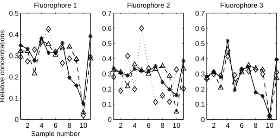
2U) or CDA-PARAFAC loadings (rc 2CDA). Fluorophore r_2Uc rc_2CDA. 1 6.6 5.6 2 26 4 3 7.3 8.2

Results for the concentration mode are presented in table 8 and figure 11.

In-455

ner filters and CDA correction have little effects on the profile of fluorophore

456

1 (rc

2U = 6.6% and r2CDAc = 5.6%) and 3 (rc2U = 7.3% and rc2CDA= 8.2%). On

457

the opposite, fluorophore 2 is far more affected. The concentration profile

esti-458

mated by U-PARAFAC is clearly unsatisfying (rc

2U = 26%). CDA-PARAFAC

459

provides an acceptable estimation as the error term decreases to 4 % . Finally

Fig. 10. Illustrations of I2R, I2U and I2CDAfor samples 1, 4, 6 and 9 of data set 2. the three estimated profiles by CDA-PARAFAC are satisfying at the exception

461

of sample 8 and 9. At the opposite of rc

2U, r2CDAc is greater for fluorophores 1

462

and 3. This is mainly due to the larger estimation errors on samples 8 and 9.

463

464

Results for excitation mode are presented in table 9 and figure 12.

Excita-465

tion mode is the most affected mode of the decomposition as for data set 1.

466

Estimation of fluorophore 1 excitation spectrum takes a clear advantage of

2 4 6 8 10 0 0.1 0.2 0.3 0.4 0.5 Sample number Relative concentrations Fluorophore 1 2 4 6 8 10 0 0.1 0.2 0.3 0.4 0.5 0.6 0.7 Fluorophore 2 2 4 6 8 10 0 0.1 0.2 0.3 0.4 0.5 0.6 0.7 Fluorophore 3

Fig. 11. Data set 2, PARAFAC loadings of the concentration mode: R-PARAFAC loadings (solid ∗ line), U-PARAFAC loadings (dot ⋄ line) and CDA-PARAFAC loadings (dash △ line)

Table 9

Data set 2, excitation mode results. Comparison with the reference loadings among three criteria: relative error on the maximum value (%), shift (nm) and relative squared error (%)

Fluorophore Test Unc. CDA cor.

Rel. err. max. val. 18 11

1 Shift 185 15

rex 110 1.5

Rel. err. max. val. 30 20

2 Shift 20 0

rex 9.6 2.1

Rel. err. max. val. 27.5 0.2

3 Shift 10 5

rex 35 0.6

CDA-PARAFAC. Regarding shape and position, the spectrum estimated by

468

U-PARAFAC is a far cry from the reference spectrum (rex

2U = 110%). On the

469

opposite, CDA-PARAFAC provides a very good estimation (rex

2CDA = 1.5%).

470

The relative error on the maximum value is smaller (11 % against 18 %)

471

but above all, the large shift (185 nm) is brought back to 15 nm. Despite

U-472

PARAFAC estimation of fluorophore 2 spectrum is acceptable (rex

2U = 9.6%),

473

CDA-PARAFAC improves this result (rex

2CDA = 2.1%). In absence of

correc-474

tion, the double peak disappears. CDA-PARAFAC correctly restores this

fea-475

ture but the relative error on the maximum value remains high (20%). On

476

the other hand, the 20 nm shift is completely corrected. U-PARAFAC

300 400 500 600 0 0.05 0.1 0.15 0.2 0.25 Excitation (nm) Intensity (a.u.) Fluorophore 1 300 400 500 600 0 0.05 0.1 0.15 0.2 0.25 0.3 0.35 Fluorophore 2 300 400 500 600 0 0.05 0.1 0.15 0.2 0.25 0.3 Fluorophore 3

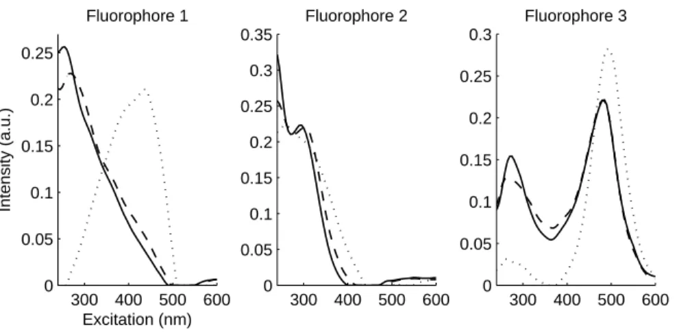
Fig. 12. Data set 2, PARAFAC loadings of the excitation mode: R-PARAFAC load-ings (solid line), U-PARAFAC loadload-ings (dot line) and CDA-PARAFAC loadload-ings (dash line)

tion of fluorophore 3 spectrum is not satisfying (rex

2U = 35%). One of the two

478

peaks almost disappears while the second one is overestimated. Nevertheless,

479

its estimation by CDA-PARAFAC is almost identical to the reference

spec-480

trum (rex

2CDA = 0.6%). The relative error on the maximum value is significant

481

with U-PARAFAC (27.5%) but it becomes negligible with CDA-PARAFAC

482

(0.2%). The shift is also reduced from 10 nm to 5 nm.

483

Table 10

Data set 2, emission mode results. Comparison with the real spectra among Compar-ison with the reference loadings among three criteria: relative error on the maximum value (%), shift (nm) and relative squared error (%)

Fluorophore Test Orig. Corr.Dil. Rel. err. max. val. 13 12

1 Shift 40 25

rem 21 4

Rel. err. max. val. 21 1.8

2 Shift 60 10

rem 63 6

Rel. err. max. val. 5.2 1.4

3 Shift 20 10

rem 8.8 0.9

Results for emission mode are presented in table 10 and figure 13. Estimation

484

of fluorophore 1 emission spectrum by U-PARAFAC is mitigated (rem

2U = 21%).

485

CDA-PARAFAC overall result is very acceptable (rem

2CDA = 4%). The

spec-486

trum is overestimated by both U-PARAFAC (relative error to the maximum

350 450 550 650 0 0.05 0.1 0.15 0.2 0.25 0.3 0.35 Emission (nm) Intensity (a.u.) Fluorophore 1 350 450 550 650 0 0.05 0.1 0.15 0.2 0.25 0.3 0.35 Fluorophore 2 350 450 550 650 0 0.05 0.1 0.15 0.2 0.25 0.3 0.35 Fluorophore 3

Fig. 13. Data set 2, PARAFAC loadings of the emission mode: R-PARAFAC loadings (solid line), U-PARAFAC loadings (dot line) and CDA-PARAFAC loadings (dash line)

value of 13%) and CDA-PARAFAC (12%). On the opposite, CDA-PARAFAC

488

limits to 25 nm the large shift (40 nm) observed when no correction is

ap-489

plied. Fluorophore 2 spectrum is more severely affected by inner filter

ef-490

fects. CDA-PARAFAC provides a very satisfying estimation of this spectrum

491

(rem

2CDA = 6%) in respect to U-PARAFAC result (rem2U = 63%). The relative

492

error to the maximum value observed with U-PARAFAC is important (21%)

493

but it is well corrected by CDA-PARAFAC (1.8%). In the same way, the 60

494

nm shift is limited to 10 nm. Fluorophore 3 spectrum is correctly estimated

495

by U-PARAFAC (rem

2U = 8.8%). CDA-PARAFAC still improves the

estima-496

tion (rem

2CDA = 0.9%). The relative error to the maximum value is lower (1.4%

497

against 5.2%) and the shift is reduced from 20 nm to 10 nm.

498

CDA-PARAFAC results on data set 2 are also conclusive. All the loading are

499

indeed correctly estimated. Relative concentrations of only one fluorophore in

500

only two samples out of eleven are poorly estimated and all the estimated

spec-501

tra are close enough to the corresponding reference spectra. The crucial point

502

on this second example is that in a real case situation of DOM tracing,

CDA-503

PARAFAC would probably give interpretative results while the uncorrected

504

FEEM would provide misleading estimations. Moreover, excitation spectra of

505

fluorophores 1 and 3 illustrate the two main kinds of spectral deviations due

506

to inner filters. Fluorophore 1 shape is distorted and its position is shifted

507

from 275 nm to 480 nm. On the opposite, the position of fluorophore 3 is

508

unchanged, its global shape is almost correct but the respective magnitude

509

of its two peaks is largely modified. CDA-PARAFAC provides an impressive

510

correction of both deviations.

511

Actually, CDA-PARAFAC appears to be a critical improvement of U-PARAFAC

512

or even ACA-PARAFAC in the case of strong inner filter effects.

5 Conclusion

514

It is possible to correct inner filter effects by using simply a controlled dilution

515

approach (CDA). This analytical solution is better than usual absorbance

cor-516

rection and quicker and safer than strong dilution, under absorbance of 0.3.

517

It has been demonstrated in this work the good ability of CDA and

CDA-518

PARAFAC in the case of standard mixtures of two fluorophores and in the

519

case of real DOM samples. In this study, CDA performed very well for

solu-520

tion absorbances up to 1.83. Further investigation should be made outside this

521

range. We conjecture that an other theoretical model of fluorescence

measure-522

ment should be used for absorbance higher than 2.

523

In respect to the PARAFAC decomposition, better results were obtained on

524

the spectral loadings. We have also highlighted the limit of ACA for the

cor-525

rection of strong filter effects. Consequently, we recommend the use of CDA

526

for FEEM experiment and PARAFAC pretreatment to avoid error and

misin-527

terpretation.

528

References

529

[1] B. Valeur, Molecular Fluorescence. Principles and Applications, Wiley-VCH,

530

Weinheim, 2002.

531

[2] A. Hansch, D. Sauner, I. Hilger, J. B¨ottcher, A. Malich, O. Frey, R. Br¨auer and

532

W.A. Kaiser, Academic Radiology, 11 (11) (2004) 1229-1236.

533

[3] E. Sikorska, T. Gorecki, I.V. Khmelinskii, Sikorski and D. de Keukeleire, Food

534

chemistry, 96 (4) (2006) 632-639.

535

[4] G.P., Coble, Marine Chemistry, 51 (1996), 325-346.

536

[5] C.A. Stedmon, S. Markager, Limnology and Oceanography, 50 (2) (2005).

537

[6] J.R., Lakowicz, Principles of Fluorescence Spectroscopy, Plenum Press, NY,

538

1983.

539

[7] C.A. Parker, W.J. Barnes, The analyst, 82 (1957) 606-618.

540

[8] J.J. Mobed, S.L. Hemmingsen, J.L. Autry, and L.B. McGown, Environmental

541

Science and Technology, 30 (10) (1996) 3061-3065.

542

[9] J.F. Holland, R.E. Teets, P.M. Kelly and A. Timnick, Analytical Chemistry, 49

543

(6) (1977) 706-710.

544

[10] C. M. Yappert and J.D. Ingle, Applied Spectroscopy, 43 (5) (1989) 759-767.

545

[11] S.A. Tucker, V.L.Amszi, W.E. Acree, Journal of Chemical Education, 69 (1992).

[12] B.C. MacDonald, S.J.Lvin and H. Patterson, Analytica Chimica Acta, 338

547

(1997) 155-162.

548

[13] A. Credi, and L. Prodi, Spectrochimica Acta Part A, 54 (1998) 159-170.

549

[14] J. Riesz, J. Gilmore, P. Meredith, Spectrochimica Acta part A (2004).

550

[15] T. Ohno, Environmental Science and Technology, 36 (4) (2002) 742-746.

551

[16] D.M. MacKnight, E.W Boyer, P.K. Westerhoff, P.T. Doran, T. Kulbe and D.T.

552

Andersen, Limnology and Oceanography, 46 (2001) 38-48.

553

[17] F. Cuesta Sanchez, S. Rutan, M. Gil Garcia and D. Massart, Chemometrices

554

and Intelligent Laboratory Systems, 36 (1997) 153-164.

555

[18] A. Garrido Frenich, D. Picon Zamora, J. Martinez Vidal and M. Martinez

556

Galera, Analytica Chimica Acta, 449 (2001) 143-155.

557

[19] J. Boehme, P. Coble, R. Conmy and A. Stovall-Leonard, Marine Chemistry, 89

558

(2004) 3-14.

559

[20] J.M. Andrade, M.P. Gomez-Carracedo, W. Krzanowsky and M. Kubista,

560

Chemometrices and Intelligent Laboratory Systems, 72 (2004) 123-132.

561

[21] R.A. Harshman, UCLA Working Papers in Phonetics, 16 (1970) 1-84 (UMI

562

Serials in Microform, No. 10,085).

563

[22] R. Bro, Chemometrics and Intelligent Laboratory Systems, 38 (1997) 149-171.

564

[23] C.A. Stedmon, S. Markager and R. Bro, Marine Chemistry, 82 (3-4) (2003)

565

239-254.

566

[24] R.D. Holbrook, J.H. Yen and T.J. Grizzard, Science of The Total Environment,

567

361 (1-3) (2006) 249-266.

568

[25] X. Luciani, S. Mounier, H.H.M. Paraquetti, R. Redon, Y. Lucas, A. Bois, L.D.

569

Lacerda, M. Raynaud and M. Ripert, Marine Environmental Research, 65 (2)

570

(2008) 148-157.

571

[26] D. Baunsgaard, Department of Dairy and Food Science, The Royal Veterinary

572

and Agricultural University, (1999).

573

[27] G.G. Anderson, K.D. Brian and K.S. Booksh, Chemometrics and Intelligent

574

Laboratory Systems, 49 (1999) 195-213.

575

[28] O. Divya and A.K. Mishra, Analytica Chimica Acta, 630 (2008) 47-56.

576

[29] P. John, I. Soutar, Analytical Chemistry, 48 (1976) 520-524.

577

[30] D. Patra and A.K. Mishra, Analyst, 125 (2000) 1383-1386

578

[31] R.A. Harshman, UCLA Working Papers in Phonetics, 22 (1972) 111-117 (UMI

579

Serials in Microform, No. 10,085).

580

[32] N.D. Sidiropoulos and R. Bro, Journal of Chemometrics, 14 (3) (2000) 229-239.

[33] N.M. Faber, R. Bro and P.K. Hopke, Chemometrics and Intelligent Laboratory

582

Systems, 65 (2003) 119-137.

583

[34] G. Tomasi, R. Bro, Computational Statistics & Data Analysis, 50 (7) (2006)

584

1700-1734.

585

[35] P. Paatero, Chemometrices and Intelligent Laboratory Systems, 38 (2) (1997)

586

223-242.

587

[36] R.A. Harshman and M.E. Lundy, Computational Statistics & Data Analysis,

588

18 (1994) 39-72.

589

[37] C. Andersen, R. Bro, Journal of Chemometrics, 17 (2003) 200-215.

590

[38] R.G. Zepp, W.M. Sheldon and M.A. Moran, Marine Chemistry, 89 (2004) 15-36.

591

[39] C.A. Andersson and R. Bro, Chemometrics and Intelligent Laboratory Systems,

592

52 (2002) 1-4.

593

[40] R. Bro and H.A.L. Kiers, Journal of Chemometrics, 17 (2003) 274-286.