Performance des réseaux de capteurs sans fil pour la transmission de données multimédia dans le contexte des lampadaires intelligents

(1)

UNIVERSITÉ DU QUÉBEC

MÉMOIRE PRÉSENTÉ À

L'UNIVERSITÉ DU QUÉBEC À TROIS-RIVIÈRES

COMME EXIGENCE PARTIELLE DE LA MAÎTRISE EN GÉNIE ÉLECTRIQUE

PAR

GHASSEN GADHOUM

PERFORMANCE DES RÉSEAUX DE CAPTEURS SANS FIL POUR LA TRANSMISSION DE DONNÉES MULTIMÉDIA DANS LE CONTEXTE DES

LAMPADAIRES INTELLIGENTS

(2)

Université du Québec à Trois-Rivières

Service de la bibliothèque

Avertissement

L’auteur de ce mémoire ou de cette thèse a autorisé l’Université du Québec

à Trois-Rivières à diffuser, à des fins non lucratives, une copie de son

mémoire ou de sa thèse.

Cette diffusion n’entraîne pas une renonciation de la part de l’auteur à ses

droits de propriété intellectuelle, incluant le droit d’auteur, sur ce mémoire

ou cette thèse. Notamment, la reproduction ou la publication de la totalité

ou d’une partie importante de ce mémoire ou de cette thèse requiert son

autorisation.

(3)

UNIVERSITÉ DU QUÉBEC

À

TROIS-RIVIÈRES

MAÎTRISE EN GÉNIE ÉLECTRIQUE (M. Sc. A.)

Programme offert par l'Université du Québec

à

Trois-Rivières

PERFORMANCE DES RÉSEAUX DE CAPTEURS SANS FIL POUR LA TRANSMISSION DE DONNÉES MULTIMÉDIA DANS LE CONTEXTE DES

LAMPADAIRES INTELLIGENTS

PAR

Ghassen GADHOUM

Prof. Adam W. Skorek, Directeur de recherche

Prof. Habib Hamam, évaluateur

Prof. François Nougarou, évaluateur

Université du Québec à Trois-Rivières

Université de Moncton

(4)

Résumé

Nowadays, wireless sensor network technology has become extremely vital in a

variety of domains because it has become necessary in many areas where the

use of this advanced technology has evolved into not only optional but also a

mandatory need, for example, in the health environment or for military use.

Indeed, there is many different technologies of wireless sensors that vary in their

use, such as Zigbee wireless sensor systems, they are more efficient in terms of

energy consumption, or a sensor Wireless networks that offer higher data rates

and improved performance. They also have their particular field of application

.

Thanks to technological developments related to sensor design and intelligent

programs embedded in their electronic circuits

,

Wireless Sensor Networks

(WSN) have become crucial in several areas of use (industry

,

health

,

space

,

military, etc.).

ln the context of this thesis, we are interested in networks of wireless sensors in

the context of multimedia data. There are several technologies related to

streaming multimedia signais in a WSN. The choice guided by several factors

including: video compression technique, network topology and wireless channels

related to the physical location of the sensors

.

The solutions currently available

(5)

The aim of this research project is to design and simulate numerous WSN

topologies for the transmission of video data in the context of intelligent

streetlights

. The routing method will be compared to find out which configuration

is the best choice to achieve the required throughput and to meet specific

deploymen

t

constraints

.

Network simulations will be carried out to validate the

theoretical study.

On the other hand,

the research approach chosen for this M.Sc.A. project in

electrical engineering is fundamentally a primary-based research, while including

some aspects of research based on previous results and work, as we will design,

model and test different topologies of wireless sensor networks.

ln addition, for

this final project, quantitative and qualitative approaches will be

used and, fundamentally

,

the project will be based on a primary research aspect.

This M.Sc.A. thesis consists of five chapters

.

At the outset,

the introductory

chapter where the research subject will be presented in a general way, then the

literature review chapter that will highlight the important theoretical points that will

be necessary to accomplish this project. This chapter will provide a theoretical

view of the need for the Wireless Sensor Network as weil as a theory behind

various technologies, such as WSN and routing protocols.

Then

,

in the Results and Discussion chapter, the main relative results of the

research will be discussed; Then

,

as a result of these analysis, we can conclude

(6)

whether the and routing protocols and number of nodes used in the WSN for

intelligent street lights affects network operation and performance. This chapter

will also include some figures and tables that will be presented to show the

results of the test and simulation steps

.

And finally, in the conclusion chapter

,

a summary of what has been do ne

throughout this report will be presented; So some recommendations that could

improve the performance of WSN for intelligent streetlights will be provided

,

Thus

this willlikely help further research in the WSN field.

(7)

Acknowledgment

1 would like to express the deepest appreciation to my supervisor Professor Adam Skorek for his crucial help and continuous support throughout this M.Sc.A. dissertation.

Besides, 1 would like to thank Ali my professors and the graduate study program directors especially Professor Mamadou Lamine Dombia and Professor Daniel Massicotte for their precious advices and worthy suggestions that made my work much better and which considerably helped me to finish my final project on time.

Correspondingly, 1 am indeed truthfully thankful to my whole family especially my parents and my brothers. Finally, 1 do honestly thank ail my friends and ail people who supported me to achieve my goals.

(8)

Scenario 3: Comparaison entre les deux technologies Wi-Fi et Zigbee avec Topologie Maillé (Mesh) 50 nœuds (avec AODV comme protocole de routage) ... 195 Scénario 4 : Comparaison entre topologies (Topologie d'étoiles, topologie de maille et topologie de ligne) 11 noeuds (Wi-Fi) AODV ... 197 Scénario 5 : Influence du nombre de nœuds sur la performance: comparaison du nombre de nœuds différents pour la topologie Mesh (11 noeuds, 20 noeuds, 50 nœuds) (Wi-Fi) (AODV) ... 199 Conclusion ... 202

(11)

List of tables

Tableau 4.1 Resolution and bandwidth of different video Formats [5] ... 44

Table 4.2 : Scenario 1 Configuration table ... 45

Tableau 4.3 Scenario 2 Configuration table ... 53

Tableau 4.4 Scenario 2 Results ... 55

Tableau 4.8 Scenario 5 Number of Nodes Vs Average Delay ... 199

(12)

List of Figures

Figure 1 Evolution of sensor during last decades [4] ... 18

Figure 2 An Exemple of a WSN Application in lOT Internet of Things [1] ... 22

Figure 3 Path discovery process of the AODV routing protocol [1] ... 26

Figure 4 Wireless Sensor Network Topologies [3] ... 30

Figure 5 Fundamental Architecture of the Network Simulator NS [14] ... 36

Figure 6 directory structure under NS2 ail in one Package[14] ... 39

Figure 7 A first Network topology [14] ... 41

Figure 8 a TCl script part 1 [14] ... 42

Figure 9 a TCl script part 2 [14] ... 43

Figure 10 Topology of the scenario 1 (50 nodes) with different routing protocols (AODV, DSR, DSDV) (Wi-Fi) ... 46

Figure 11 Throughput comparison between Different Routing Protocols (AODV, DSDV, DSR) ... 47

Figure 12 Jitter comparison between Different Routing Protocols (AODV, DSDV, DSR) ... 49

Figure 13 End to End Delay comparison between Different Routing Protocols (AODV, DSDV, DSR) ... 51

Figure 14 Topology of the scenario 1 (50 nodes) with different video formats (CIF, 4CIF, QCIF ... ) with DSDV routing Protocol ... 54

Figure 15 Throughput : Mesh Topology 50 nodes (Wi-Fi) Comparaison between different video formats with DSDV routing Protocol ... 56

Figure 16 Jitter: Mesh Topology 50 nodes (Wi-Fi) Comparaison between different video formats with DSDV routing Protocol ... 58

Figure 17 End to End Delay : Mesh Topology 50 nodes (Wi-Fi) Comparaison between different video formats with DSDV routing Protocol ... 60

Figure 18 The scennario's topology (Wi-Fi) ... 63

Figure 19 The scennario's topology (Zigbee) ... 64

Figure 20 Throughput : Wi-Fi Result vs Zigbee Result 50 nodes Mesh Topology (with AODV) ... 65

Figure 21 End to End Delay : Wi-Fi vs Zigbee et Figure 22 End to End Delay: Wi-Fi vs Zigbee ... 67

Figure 24 Mesh Topology 11 nodes (Wi-Fi) AODV ... 70

Figure 25 Star Topology 11 nodes (Wi-Fi) AODV ... 70

Figure 26 Throughput Comparison between topologies (Star Topology, Mesh Topology and li ne topology) 11 nodes (Wi-Fi) AODV ... 72

(13)

Figure 28 End to End Delay Comparison between topologies (Star Topology,

Mesh Topology and line topology) 11 nodes (Wi-Fi) AODV ... 77

Figure 29 Network Topology Mesh Topology 11 nodes ... 80

Figure 32 Bar Chart : Number of Nodes vs Average Delay ... 199

Figure 33 Bar Chart : Number of Nodes vs Throughput ... 201

Figure 34 Throughput : Influence of the number of nodes on the performance (Wi-Fi) (AODV) ... 82

Figure 35 Jitter : Influence of the number of nodes on the performance (Wi-Fi) (AODV) ... 84

Figure 36 End to End Delay: Influence of the number of nodes on the performance (Wi-Fi) (AODV) ... 86

(14)

Chapter 1 : Introduction

1.1. Overview

Nowadays Wireless sensor Networks technology has become tremendously vital

in a diversity of aspects

,

since

,

it has become intensively necessary in many

different domains where the use of this cutting edge technology turned out to

become not only an option but crusial

,

whether in ordinary ut

i

lization

,

in health

environ ment or in Military use. Indeed

,

there is numerous diverse sorts of

Wireless sensor Technology

,

that differs regarding the domain of use

,

such as

Zigbee Wireless Sensor Networks who are better for energy comsumption

eff

i

ciency

,

or Wi-Fi Wireless Sensor Networks who offers higher data rates and

enhanced performance

,

ail of them have its special domain of application.

Apart from this introductory chapter

,

this dissertation will contain three more

chapters. Initially the literature review chapter which is going to underl

i

ne and

stress the diverse significant theoretical and background points that will be

required to accomplish this M

.

Sc

.

A

.

final project

,

and which have been utilized in

this research project

,

this chapter will give a theoretical point of view of the need

behind the Wireless Sensor Network as weil as some theory behind diverse

WSN technologies

,

especially the routing protocols

.

(15)

made such as whether or not the number of nodes utilised in the WSN affects the

Network performance

,

And what routing protocol is performing better and so on

and so forth, also

,

this chapter will enclose some figures and tables which will be

presented to show the result of the testing and simlation steps

.

And finally, in the

conclusion chapter

,

a summarise of what was performed throughout this report

will be presented

;

then

,

some recommendations which might improve the

performance of the WSN

,

will be given

,

so that

,

it probably will help to achieve

further research in the domain of WSN.

1.2. Project aims and objectives

The aim of th

i

s M.Sc.A. Project is to design and simulate different WSN

topologies for the transmission of video data in the context of intelligent

streetlights

.

Routing methods will be compared to achieve the required

throughput and to meet specific deployment constraints

.

Network simulations will

be carried out to validate the theoretical study

.

1.3. Research Approach

For this final project

,

the research approach is basically a primary based

research whilst it will include some second based research aspects as we are

going to design

,

build and test a different Wireless sensor Network topologies.

(16)

ln addition, scientific research is defined as: studying a subject in detail for

discovering new information or to find out a new interpretation [12]. Moreover, for

this final project both quantitative and qualitative approaches will be utilized and

basically, the project will be found on a primary research aspect.

(17)

Chapter 2 : Literature Review

Like many other technologies Wireless Sensor Networks is the fruit of continuous effort and research lead by military research institutions, for instance, in 1978 during the distributed Sensor Nets workshop arranged by DARPA [1], The aim of this workshop was to foster research and innovation in the domains related to sensor networks such as distributed programs and signal processing [1] .

Then in 2001, the notion of Wireless Integrated Network Sensors (WINS) was introduced by the university of California with cooperation of Rockwell Science center [1].

The smart sensing system is composed by a digital signal processing circuit, interface circuits wireless radio,microcontroller, integrated multiple sensors and a CMOS chip [1].

ln addition a WSN Project called the smart dust project at the university of California at Berkeley aimed to invent a very tiny sensor nodes termed mote [1]. The purpose of this research was to show that very small devices such as the size of a dust particle or a grain of sand are fully capable to include a thorough sensor system.

(18)

ln 2000 Rabaey et al. worked on the PicoRadio project which aimed to design a

low-power wireless sensor instruments, that consume energy in a significantly

very low rate and which are able to get energy autonomously from the

functioning environ ment like solar energy [1].

And in 2005 Calhoun et al concentrated on the MIT IJAMPS project which

highlighted low-power for sensor nodes in two aspects, material and program. It

involved the utilization of dedicated microcontrollers for data processing methods

and for active voltage scaling in order to decrease power consumption in terms

of the software side [1]

.

Even though most of the research work has been done by academic

organisations and universities, throughout recent years, numerous startups and

firms utilized on WSN have emerged and contributed on fostering this research

field. For instance Ember Corporation, Oust Networks, Sensoria are some of

these companies [1].

These firms offers the option to buy WSN instruments that fits the different real

life needs with various programming and data management options [1]

.

(19)

.

_{. .}

Figure 1 Evolution of sensor during last decades [4]

2.1. WSN Applications

00

.

o

.

_.

,

o

.

,

1

,

.

_.

,

• WSN have different kind of applications in several domains su ch are health,

Military

,

national security and the Internet of things

(20)

2.1.1 Health

Health Problems related to modern life style have risen during the last decades

and the need to get a technological solution has also increased. One of these

solutions is WSN [1].

A research on heart diseases made at Framingham institute came to the

conclusion that many cardiovascular diseases can be avoided due to physical

activities [1]. And a new publication proved that around 10 percent of the total

number of deaths in 2008 are caused by lack of activity [1].

Recent research acclaims 150 minutes of sport every week for adults. But about

33 %

of adults do not practice enough training and sport, thus these people are

significantly more vulnerable to diabetes and cardiovascular diseases [1].

Eating habits have altered throughout the last fi

ft

Y years. Aiso the popularity of

fast and processed foods increased steadily, those kinds of foods contains more

amount of fat salt and sugar.

Meals based on meat has become very common, and the consumption of

vegtables and fruits declined

,

thus

,

the amount of calories rose triggering

increase obesity and diseases related to it.

(21)

Ali these health problems mentioned above

,

have to be tackled by research and

technologies

,

where cams the need to WSN in this filed

.

For instance wireless

sensors can be connected with the patient's organs and send information to the

doctors in real time

.

2.1.2 National Security

Nowadays national security risk of non-classical crimes

,

is considered as a

steady issue for both citizens and governments

,

These dangers vary from

chemical and biological to even nuclear and radiological.

Unceasing observing and extra caution is consequently needed to thwart these

kind of threats

.

Even though detection methods which relies on laboratory analysis shows

outstanding sensitivity and results

,

these laboratory are usually far away from the

menace zone

,

therefore

,

this many cause many issues such as substantial

delays and struggle

i

n terms of information gathering

.

Hence the fundamental need of wireless sensors deployed in the threat zone and

able to gather information promptly and send it in real time to the laboratory or

the research institutions

.

(22)

ln this case WSN are required to identify risks in different places and conditions

,

su ch as on land or in air and so on.

2.1.3 The Internet of Things

The Internet of things has bounded our lives in a variety of ways. Thanks to

ubiquitous internet connectivity

,

and sophistication in Information technologies

,

loT has become a de facto need for many individuals, institutions and

companies.

This fact will change drastically the life style of many human being in many

aspects like distraction

,

employment and education

.

WSNs contribute significantly in interacting with the outside world,

Like many other technologies loT is not an exception in the sense that its

success depends on binging perceptible advances and enhancements to human

being.

It is expected that WSN are going to be vital in del

i

vering data flows

,

that loTs

projects will be developed.

(23)

.- • • •• ·

P

h

ys

i

cal quan

ti

ties

•••• ,

Protein Bacteria

:

~.;~

W

~ Electrtcal signai ~ -Measurement~ ~

0,

Sound

_Transduction

,

optlcal signai , Motion

'.

--

-

----

Chemical

Figure 2 An Exemple of a WSN Application in 10 T Internet of Things [1 J

2.2. Rooting Protocols

2.2.1 DSR

ln 1994 Johnson introduced the DSR, DSR stands for Dynamic source routing,

and it uses what is called "route discovery" and "route maintenance" technics.

ln DSR every node preserves a path cache with new information that changes

constantly when node acquires new paths.

Anode willing to direct a packet will primarily examine its route cache to find out

if it previously had a route to the end point. And this is alike the AODV protocol.

(24)

discovery procedure through a path request packet, which encloses the

destination's address, the source's address and a sole application ID.

When the request spreads across the network, every node enclosures its

particular address inside the application packet prior re-spreading it.

As a result, a request packet registers a path containing the entire nodes it has

cali on. And once anode gets a request packet and discovers its sole address

logged in the packet, it throw-outs this packet and stop spreading it more.

A node preserves a cache of freshly forwarded application packets; saving their

sender request unique IDs and addresses, and rejects every identical request

packets.

When a request packet reaches its endpoint, it will save the whole route from the

source to the endpoint.

ln what so-called

"symmetric

network", the target node is able to unicast an

answer packet, covering the gathered path information, back to the source node

using the rigorous identical route as used by the request packet.

(25)

As soon as the reply packet reaches the source, the source node will be able to

save the novel path inside its cache and begin conveying packets to the

endpoint.

The DSR routing protocol, is also alike the AODV in another point

,

they both

retains a path conservation method founded on error messages,

that are

produced when the link layer senses a communication breakdown because of an

interrupted link.

Each packet in DSR conveys path information, unlike AODV. This advantage of

DSR over AODV permits to in-between nodes (Between source and destination)

to insert novel paths preemptively to their personal caches

.

2.2.2 AODV

Ad hoc on- Demand Distance Vector (AOVC) Protocol was invinted by Pekins

And Royer in 1999.

Nodes do not preserve routing details and do not contribute in cyclic routing table

(26)

AODV utilizes what so called broadcast route finding method. When the source

lacks routing details in its table, the AODV's route finding procedure, is started

when a source node wants to send data to alternative node.

ln order to do this, the source node transmits a route request (RREQ) packet to

other nodes that are near it, these nodes encloses the addresses of the endpoint

and the source, the hop total value, a transmission ID and dual sequence

numbers.

The transmission ID will be increased by one when the source node discharges a

novel RREQ packet that is joined to the address of the source node in order to

solely identify a route request.

As soon as anode obtains a route request packet,

anode

,

which owns an

existing path to the endpoint node, replies by transferring a route reply (RREP)

message straight to the node that was behind the launching of the route request

(RREQ)

.

Then, the route request is resent by the node to its in-between neighbors. Thus

an identical route request (RREQ) is rejected.

(27)

Every node in the topology preserves its private sequence number. And If a

source node delivering a route request packet it already have its specifie

sequence number

.

Therefore, In-between nodes do not respond to a RREQ unless the sequence

number of their path to the endpoint node is (>=) greater than or equal to the

endpoint order number stated in the route request packet.

Whenever a route request is resent, the in-between node saves the neighbor

'

s

node location, from which the route request was obtained, thus creating an

opposite route from the source node to the end point node.

When the Route Reply return to the source node, every in-between nodes

establish a forward pointer toward the node where the Route reply was received

and registers the lates which the RREP

Source

o

Destination

o

RREQ Packet Propagation Path Taken By RREP Packet

Figure

3

Path discovery pro cess

of

the AOOV routing proto col

[1].

(28)

nodes after multiple hops [1].

The lifecycle of unutilized routes is reduced using a timer embedded in every

node

'

s routing table.

A

"

Hello Message

"

is regularly swapped to show how their links are performing.

Throughout the process

,

whenever a link interrupts

,

the midway node near to the

source

,

detects the problem and sends to the source what is called a route error

packet.

As soon as the source obtains a route error packet, it refreshes the path

discovery procedure

.

With the AODV routing protocol

,

routes are solely created when required

,

which

helps significantly to optimize route table and to prevent unnecessary updates

and interactions with unused routes.

Whilst

,

AODV needs regularly to swap the

"

Hello messages

"

with other nodes

that are close to it.

(29)

ln the case of the reverse path, the route created between the source and

destination is the opposite route, thus AODV routinhg protocol considers that ail

paths are symmetric.

2.2.3 DSDV

Destination-Sequenced Distance-Vector Routing (DSDV) is a table driven routing

protocol created by C. Perkins and P.Bhagwat in 1994. It was based on the

distributed Bellman-Ford algorithm. Each Node keeps a list of distances for every

destination through each neighbor [1]

.

This data is kept in a routing table with an order number that shows every

access.

The aim of the sequence numbers is to permit nodes to recognize old routes

from recent on es to avoid routing loops.

ln this routing algorithm each node send refreshes to the routing table regularly,

(30)

DSDV utilizes two kinds of packets to show its routing table

. "

Full dump

"

comprises ail obtainable routing information

,

and

"

incremental packet

"

comprises

solely data that has altered after the final

"

Full dump

".

The

"

Incrementai packet

"

when acquired bya node

,

the information of the former

and the later are checked

,

then if the packet's route features a newer sequence

number, the equivalent route in the node

'

s table will be changed

.

And if the order numbers are the same and the packet's route possesses a tinier

interval, in this case a packet's route will substitute the node

'

s route

.

(31)

2.3. Wireless Sensor Network Topologies

Star

Pair

Cluster tree

Mesh

Coordinators Routers

o

End devices Figure 4 Wireless Sensor Network Topologies [3]

Wireless sensor networks can have several network topologies that dictates the

way the radio signais are rationally related together

,

however their physical

disposition can seem dissimilar, the figure above highlights three main

topologies

:

Pair, Mesh and Star [3].

2.3.1 Pair Topology

It is the most basic and simple topology, one node is the coordinator, and the

(32)

2.3.2 Star topology

This topology is quite commonly used; the source node or what is also called the

coordinator node is in the middle and it connects ail other surrounding nodes.

Every message in the network must go via the coordinator node that routes them

according to the requirements. In addition

,

the end nodes are not able to

exchange information straightforwardly. First, they must communicate with the

coordinator node [3]

.

2.3.3 Mesh Topology

The Mesh topology is also very common

,

and it utilizes router nodes and the

coordinator node. Not like in the case of the star or the pair topology, the

coordinator nodes can pass messages to the end nodes via the router nodes [3].

The Coordinator node is actually a particular shape of router,

its aim is to

administer the WSN. Besides

,

it is able to route messages [3]

.

2.3.4 Cluster tree Topology

ln this topology the network is divided into clusters and routers are considered

like the backbone of the network, and the end nodes grouped around each router

(33)

2.4 Related Work

To find out the most efficient rooting protocol for Vehicular Ad-hoc Network A

comparison between three rooting protocols (AODV, DSDV, DSR) was done, the

comparison metrics were: average throughput, delay, PDR and energy

consumed [15]

.

DSDV had the worst performance and AODV reached the

highest throughput and DSR showed a good performance with the lowest delay

[15]. Three rooting protocols (AODV, OLSR

,

ZRP) are compared to find out the

security issues of Zigbee (IEEE 802.15.4) standard against what is called the

wormhole attack [16].

And the metrics utilized were end to end delay, throughput, Packet delivery ratio

PDR and energy consumption and they used Qualnet Simulator 5 as a simulation

tool [16].

Assesses the precision estimating the distance between the source and

destination nodes for AODV routing protocol in MANET using statistical and

neural network models [17]. And they concluded that neural networks

outperformed other models such as statistical models and ARIMA model [17].

Highlighted the security aspec

t

of the AODV routing protocol in VAN ET, they

tried to improve the AODV algorithm in order to overcome the Black Hole Attack

[18]. Thus an algorithm is suggested tha

t

can foster the AODV

'

s security by

detecting the black Hole Attacks. Source node saves the route responses in a

table [18].

(34)

[19] Focused on analyzing the routing performance in the context of robotics

.

They performed a profound performance comparison between numerous ad hoc

routing protocols.

[20] Numerous routing approaches were compared in wireless mesh networks.

they attempted to boost routing algorithms and connection metrics

ln most of the cases not the best route is chosen due to the routing protocol's

issues, interflow interference or inaccurate link metric design [20].

[21] Focused on analyzing the routing protocols for the emergency perspective

,

many routing approaches were compared such as proactive and reactive routing

protocols

,

to find out which ones are the best for the emergency case scenario

.

A metropolitan zone was selected, and three routing protocols were compared

AODV, CBRP and DSDV via NS2 network simulator [21]

.

[22] Compared between performance metrics of AODV and DSDV routing

protocols for Mobile Ad hoc Network, Throughput

,

PDR and routing overhead of

both rout

i

ng protocols were analyzed. [22] came up to the conclusion that, for the

scenarios analyzed

,

the AODV

'

s Performance is superior than DSDV.

However they showed that the performance of AODV decreases significantly

when it faces the black hole attack. And they proposed a modified AODV

algorithm that can deal better with that kind of attacks [22].

(35)

[23] Compared between performance metrics of DSR, AODV, OLSR and DSDV routing protocols for MANET (Mobile Ad hoc Network), Throughput, PDR, delay and routing overhead of the above routing protocols were analyzed via NS2.

[24] proposed a modified version of AODV named irresponsible (iAODV). This routing technique is a probabilistic forwarding suggested by [25] .

[24] found out that iAODV had better performance than AODV in terms of overhead traffic, as it decreased it considerably throughout the route discovery stage.

(36)

Chapter 3 : Simulation Toois and environment

NS2 or Network Simulator 2, is basically an event driven simulation software that is widely utilized in experimenting communication networks.

NS2 offers the ability of simulation of both wired and wireless networks as weil as

their specifie protocols [14].

NS2 was created in 1989, and since it is very flexible and composed by several units that can be added to it, NS2 has become widely well-liked in the networking society [14].

Cornell University and the university of California contributed significantly in the

evolution of the Network Simulator and in 1995 DARPA founded the

improvement of it [14].

Recently the National Science Foundation has become a contributor in the

(37)

3.1 Basic Architecture of NS2

Tel

Simulation

Script

Simulation

Trace

File

c++

i

-...

NS2 Shell Executable Command

5)

,.

"-,.

"-,

____

.A:

: __ ,

,

__

:::~

____

,

NAM

,

, Xgraph ,

: (Animation)

:

: (Plotting) :

---

-

---~

Figure 5 Fundamental Architecture of the Network Simulator NS [14]

This figure above shows the fundamental architecture of NS2. NS2 affords a

command named

"

ns

"

to run the TCl script.

For exemple to execute a TCl Script named

"

Exemple1

.

TeI

"

, we have to write

the following commend

"

ns Exemple1.TeI"

Then

,

if the commend is executed properly

,

a simulation trace file will be

generated

,

and it is essential to plot a graph and to analyse the network

behavior.

NS2 is founded around two main programming languages C++ and OTei (Object

oriented tool command languge). C++ describes the inside mechanism of the

(38)

simulation objects, the oTcI designates the outside mechanism such as planning

discrete events, building and designing the objects [14].

TclCL connects between the two programming languages (OTcl and C++).

Variables defined in a OTcI are linked to a C++ objects. These variable are

actually a string in the OTcl and does not hold any role, however the role

is

described in the linked C++ object. In OTcI, variables behaves as an interface

that communicates with users and others OTcl objects [14].

3.2 Installation

NS2 is an open source simulation tool, and it can be downloaded free of charge

from its official website nS.com

.

Even though it has been established in the UNIX

Ecosystem, NS2 is able to work on several Operating systems su ch as Unix,

Mac and Windows.

ln our case we decided to install NS2 version 2.35 on Linux Ubuntu 12.04 L TS

because it works very weil on this OS.

(39)

Table 3.1 list of Steps to install NS2

Steps Description

1- Sudo apt-get update To install necessary updates for the

operating system

2- Sudo apt-get install build essential To install the library called "Iibxmu-dev"

autoconf automake libxmu-dev on the Operating system,

3- Download NS2.35 Download the NS2 zipped file

4- tar zxvf ns-allinone-2.35.tar.gz Unzip the NS2 zipped file

5- cd ns-allinone-2.35 Access the directory of NS2

6- ./install Install NS2

7 - ./validate Check if every component is installed

properly

3.3 Directories and convention

Now NS2 is installed in directory nsallinone-2.35. The figure below illustrats the directory structure under nsallinone-2.35.

As it is shown in the figure below, they are four directory levels. Firstly, the nsallinone-2.35 directory, then in level two we find the NS2 simulation modules and the TclCL classes, next in the level three there is modules in the interpreted hierarchy and finaly in the fourth level they are the frequently utilized modules.

(40)

LEVEL 1

r-

-

---

AirNS2

-1

!

simulation \

i

modules f<:~ . . - - - l L . . . - - - - , !. _____________ . ________ 1 r-- ------- ---.,

..

. J

TclCL 1

..

-::1

classes

i

.--_...1..-_""~'/'

L ____

_

_________

j LEVEL 2

LEVEL 4 f---ë"om-riïoniy-~üsë-ëi!

___

.----_--~

!

modules in the

':::::>-

----j interpreted hierarchy [

..

_---_._---~

" __ ,

rt~;~~;d~i~-~--i-~--i "-":::'-',-1 the i ,----L_,.-- .:':'", interpreted

i

hierarchy

i

1.. ______________________ J LEVEL 3

Figure 6 directory structure under NS2 ail in one Package [14}.

3.4 Running NS2 Simulation

3.4.1 NS2 Program invocation

As NS2 Is now installed, it can be invoced using this commend UNS [filename.tcl]

[arg] "

[filename.tcl] [arg] are not compulsory arguments. In that, if the UNS" command

did not receive an argument, an NS2 domain will be invoked and NS2 will be

ready to execute orders as soon as they are written. And if in addition to the UNS"

commend the argenment U[filename.tcl)" will be given, NS2 will execute the whole

(41)

3.4.2 Main NS2 simulation steps

Table 3.2 Main NS2 simulation steps

Simulation Steps

Description

1- Design

Design of the simulation scenario

2- Write the program

Write the Tel script

3- Run, test and reconfiguration

Run the Tel script

4- Post simulation Processing

Analyse the trace file (outtr) in order to

understand the network behavior.

The table above

resumes

the main four steps of NS2 simulation, firstly in the

design step the aim and the puspose of the network should be fixed as long as

the network performance and

the

configuration, secondly the Tel script should

be written in accordance with the Network design, then in the third step the Tel

script should be runned to test it and to reconfigure it if necessary. And finally the

trace

file (outtr) should be analysed todescribe the network behavior and to

critisize its performance.

(42)

3.5 A Simulation Exemple

0

node

C".:)

Transport agent "-Application "-54 Mbps"- "'"

--

.

UDP Flow 10 ms Delay

-

_

.

_

.

_TCP_Flow

Figure 7 A first Network top%gy [14J

The figure above highlights a network design formed by five nodes. As it is

shown in the figure, nO transmit CBR traffic to node n3 and node n1 sends FTP

traffic to n4.

ln NS2 point of view CBR and FTP traffic source are transmitted by UDP and

TCP protocols through what is called

"UDP

agent" and

"TCP

agent". Whilst the

receiver are correspondingly

"Null

Agent" for UDP and

"TCP

Sink agent" for TCP.

(43)

#

myfirst_ns.tcl

#

Create a Simulator

1 s e t ns [new Simulator]

#

Create a t r a c e f i l e

2 s e t mytrace [open o u t . t r w]

3 $ns t r a c e - a l l $mytrace

#

Create a NAM trace f i l e

4 s e t myNAM [open out.nam w]

5 $ns namtrace-all $myNAM

#

Define a procedure f i n i s h

6 proc f i n i s h { } {

7

8

global ns mytrace myNAM

$ns flush-trace

9

10

11

12 13 }

close $mytrace

close $myNAM

exec nam out.nam

&

e x i t 0

#

Create Nodes

14 s e t nO [$ns node]

15 s e t n1 [$ns node]

16 s e t n2 [$ns node]

17 s e t n3 [$ns node]

18 s e t n4 [$ns node]

#

Connect Nodes with Links

19 $ns duplex-link

$nO $n2

20 $ns duplex-link

$n1 $n2

21 $ns duplex-link

$n2 $n4

22 $ns duplex-link

$n2 $n3

23 $ns simplex-link $n3 $n4

24 $ns queue-limit $n2 $n3

100Mb

54Mb

10Mb

40

Figure 8 a TeL script part 1 [14]

5ms DropTail

10ms DropTail

15ms DropTail

(44)

#

Create a UDP agent

25 set udp [new Agent/UDP]

26 $ns attach-agent $nO $udp

27 set null [new Agent/Null]

28 $ns attach-agent $n3 $null

29 $ns connect $udp $null

30 $udp set fid_ 1

#

Create a CBR traffic source

31 set cbr [new Application/Traffic/CBR]

32 $cbr attach-agent $udp

33 $cbr set packetSize_ 1000

34 $cbr set rate 2Mb

#

Create a TCP agent

35 set tcp [new Agent/TCP]

36 $ns attach-agent $n1 $tcp

37 set sink [new Agent/TCPSink]

38 $ns attach-agent $n4 $sink

39 $ns connect $tcp $sink

40 $tcp set fid_ 2

#

Create an FTP seSS10n

41 set ftp [new Application/FTP]

42 $ftp attach-agent $tcp

#

Schedule events

43 $ns at 0.05 "$ftp start"

44 $ns at 0.1

"$cbr start"

45 $ns at 60.0 "$ftp stop"

46 $ns at 60.5 "$cbr stop"

47 $ns at 61 "finish"

#

Start the simulation

(45)

Chapter 4 : Design and Implementation of the Scenarios

The purpose of this findings and discussion chapter is to present the key relative findings of the research besides explaining their meaning, thus some figures and tables will be highlighted in order to show, on one hand, Whether the wireless sensor network in the case of the intelligent lamps scenarios, is working properly or not and on the other hand, to discuss how much the results found out were similar to what was expected form a theoritical point of view.

Tableau 4.1 Resolution and bandwidth of different video Formats [5]

Format Resolution Typical BW

QCIF (114 CIF) 176x144 260K CIF 352x288 512K 4CIF 704x576 1 Mb/s SO NTSC 720x480 Analog, 4.2Mhz 720 HO 1280x720 1-8 mb/s 1080 HO 1080x1920 5-8 mb/s h.264 12+ mb/s mpg2 CUPC 640x480 max YouTube 320x240 Flash(H.264)

(46)

This Table above shows the Resolution and bandwidth of different video

Formats.

4.1 : Scenario 1 - Comparison of mesh topology 50 nodes with

different routing protocols (AODV, DSR, DSDV) (Wi-Fi)

Table 4.2 : Scenario 1 Configuration table

Simulation Tooi

Network dimension

Number of nodes

Simulation Time

Maximum queue

Data transfer mode

Maximum air data rates

Node mobility

Propagation model

NS2 Version 2.34

650 X 650

50 nodes

100 seconds

50 packets

Direct transmission

IEEE 802.11: 2000 Kbps (Wi-Fi)

off

Two-ray Ground

Rooting potocols

AODV, DSR, DSDV

Channel Capacity (Maximum Data 1 Mb/s (Mega bit per second

rate)

=

(Video Format Bandwidth)

(Mbps))

Packet size

Transfer Protocol

Data traffic

512 Bytes

UDP

CBR

(47)

~~~_3~4 _ _ _ _ ~~~~~

--

_-

•

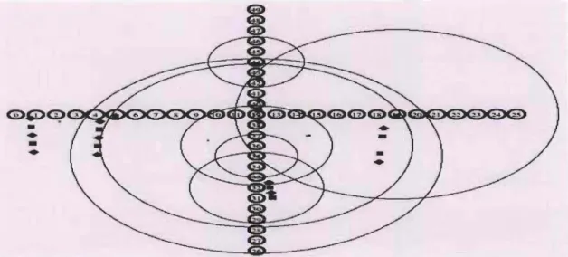
Figure 10 Top%gy of our scenario 1 (50 nodes) with different routing protoco/s (A 00 V, OSR, OSOV) (Wi -Fi)

As it is shown in the figure above the topology of the first scenario

is

composed

by 50 nodes representing the smart lights in the street they are spread on a

surface of 650 meter X 650 meter. The distance between smart lights is 25

meters (Iike in real life) and as it is outlined ln the table above, three routing

protocols is going to be tested (AODV, DSDV, DSR) in the sa me condition and in

the sa me Network configuration parameters in that, the Simulation Time is going

to be 100 seconds, the maximum queue allowed

50 packets,

the

data

transfer mode direct transmission, the maximum air data rates (IEEE 802.11:

2000 Kbps (Wi-Fi)) Node mobility will be off and the propagation model is

Two-ray Ground.

ln addition the Packet size will be 512 Bytes, Transfer Protocol will be the UDP

since it is commonly used for video transmission, and for data traffic we are

(48)

going to utilize the CBR as it is frequently used for streaming mul

t

imedia content.

And because many nodes are interconnected the topology of our network is

going to be the Mesh topology

.

4.1.1 Throughput Mesh topology 50 nodes with different routing

protocols (AODV, DSR, DSDV) (Wi-Fi)

Throughput Comparison Between Different Routing Protocols(AODV - DSDV -DSR)

1400 - -AODV - -DSDV - -DSR 1200

~

1000 'i5" c:

l

A

PA

v

"

0 ₈₀₀ (.) Q) ~ _a; 600

"'"

(.)

'"

Cl.. 400 200 0 0 10 20 30 40 50 60 70 80 90 100 Simulation Time(s)

Figure 11 Throughput comparison between Different Routing Proto cols (AODV, DSDV, DSR) -Our Result

ln this scenario we are going to compare these performance metrics

:

Throughput

,

Jitter and End to end delay of Mesh topology (50 nodes) w

i

th

different routing protocols (AODV

,

DSR

,

DSDV) in order to find out witch routing

protocol is performing bette

r.

(49)

ln the figure above we compared the throughput of different routing protocols of

nodes AODV

,

DSR and DSDV.

As it is shown in the table above

,

The setup for the simulation scenario

functioning at 1 Mbps (Data rate) for the three senarios DSDV as weil as AODV

and DSR.

As it is shown in the figure above, we notice that the highest throughput when we

utilized the AODV routing protocol, in the fi

r

st seconds of the simulation

,

it

plummeted to reach about

700

Packets per second.

Then by reaching the 4

th

second ail the routing protocls were quite steady in

around

700

packets per second

,

whilst by the

12'h

second DSR

'

s throughput rose

sudinly to reach around

1000

packets per second.

DSDV's throughput showed less stability than the others since by reaching the

35

th

second it decreased to reach

600

Packets per second then between

60

and

70

seonds it fluctuated between

800

and

700

Packets per second

.

When there is a big traffic, the collision rate escalates and this is how the

throughput of the system is affected. We observe that the highest throughput

when When AODV was utilized was around

1200

packets per second at the third

second and during most of the time of the simulation

,

the throughput remained

steady at around

700

Packets per second until the end of the simulation.

(50)

4.1.2 Jitter Mesh topology 50 nodes with different routing protocols

(AODV, DSR, DSDV)

(Wi-Fi)

Jitter of ail generated Packets(AODY - DSDY - DSR) 0.05 0.04 ... ~ c: 0 u ₀_.₀₃ QI (J) ... (J) 0; .::t: u ₀_.₀₂ ro 0.. ~ QI

-

ro 0.01 "-QI c: QI (!) ' -0 0 "-QI .;; -, -0.01 -0.02 0 0.5 1.5 Sequence Number - -AODY - -DSDY - DSR 2 2.5 X 104 Figure 12 Jitter comparison between Different Routing Proto cols (AODV, DSDV, DSR) -Our Result

The difference in the delay of received packets Is called jitter.

From a sending point of view, packets are transmitted in a steady f10w and there

(51)

Various factors such as network congestion

,

inappropriate queuing, the routing

protocol used, might cause some issues like the instability of the network data

flow, or the fluctuating variation of the delay between every packet.

This figure above shows the collective spreading of the jitter throughout the

simulation time for different routing protocols (AODV

,

DSDV and DSR) using the

same number of nodes 50 nodes.

We notice that in the scenario of the AODV routing protocol

,

at the beginning of

the simulation

,

the jitter rose drastically and reach more than 0

.

04 seconds

,

then

it steadied to become quite similar to the other two scenarios (DSDV and DSR

routing protocol)

,

and to fluctuate between 0 and 0

.

01 seconds for most of the

time

.

Moreover, comparing DSR with other routing protocols it has the most stable

jitter

,

however DSDV has the most unstable jitter amomg the three routing

protocols

,

since after about 5000 sequences the jitter reached around 0.02

seconds and after 12000 sequences it reached about 0.03 seconds and after

about 15000 sequences it reached 0

.

02 seconds and by the end the sequences

it 50tilize5050d between 0 and 0.01 seconds.

(52)

4.1.3 End to End Delay Mesh topology 50 nodes with different routing

protocols (AODV, DSR, DSDV) (Wi-Fi)

Average Simulation End2End Delays vs Throughput of Sending Bits(AODV - DSDV - DSR)

3r-~--~--~~--~--~~~=c==~~ 'Ô' § 2.5 u Q) ~ >. ~ Q)

2

o "0 c: W N "0

Ji

1.5 c: .2 (U :; E ü.i Q) en CIl

~

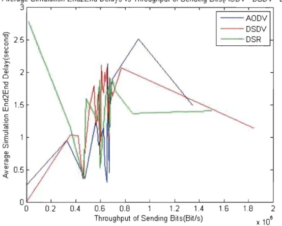
0.5 - -AODV - -DSDV - DSR 0.2 0.4 0.6 0.8 1.2 1.4 1.6 1.8 2 Throughput of Sending Bits(Bitls)

Figure 13 End to End Delay comparison between Different Routing Protocols (AODV, DSDV, DSR) - Our Result

The end-to-end delay is the time duration for a packet to be sent plus the time

duration to obtain an ac

k

nowledgment

,

in other words

,

the delay involves the

data transmission time between the two spots of signal.

ln the figure above we notice that the overall end to end delay of the DSR rout

i

ng

protocol scenario was bette

r

when we compare it

t

o the other routing

p

roto

c

ol

s.

(53)

The Analyze of the results of different routing protocols AODV, DSDV, DSR and the same topologies and the sa me number of nodes shows that the end to end network performance depends on the routing protocol that has been used.

(54)

4.2 : Scenario 2 - Mesh Topology 50 nodes (Wi-Fi) Comparaison

between different video formats (CIF, 4CIF, QCIF) with DSDV routing

Protocol

Tableau 4.3 Scenario 2 Configuration table

Simulation Tooi

Network dimension

Number of nodes

Simulation Time

Maximum queue

Data transfer mode

Maximum air data rates

Propagation model

NS2 Version 2.34

650 X 650

50 nodes

100 seconds

50 packets

Direct transmission

IEEE 802

.

11: 2000 Kbps (Wi-Fi)

off

Two

-

ray Ground

Rooting potocols

DSDV

Channel Capacity (Maximum Data 260 Kb/s

,

512 kb/s

,

1 Mb/s (Mega

rate)

=

(Video Format Bandwidth)

bit per second (Mbps))

Packet size

512 Bytes

Transfer Protocol

UDP

Data traffic

Topology

CBR

Mesh

(55)

Figure 14 Topology of the scenario 1 (50 nodes) with different video formats (CIF, 4CIF, QCIF .. .) with DSDV routing Protocol- Our Result

As it is shown in the figure above the topology of the first scenario is composed

by 50 nodes representing the smart lights in the street they are spread on a

surface of 650 meter X 650 meter. The distance between smart lights is 25

meters (Iike in real life) and as it is outlined

l

n the table above, three video

formats is going to be tested (CIF, 4CIF, QCIF) in the same condition and in the

same Netwo

r

k configuration parameters in that

,

the Simulation Time is going to

be 100 seconds, the routing protocols is going to be DSDV, the maximum queue

allowed 50 packets

,

the data transfer mode direct transmission, the maximum air

(56)

data rates (IEEE 802.11: 2000 Kbps (Wi-Fi)) Node mobility will be off and tge

Propagation model is Two-ray Ground.

ln addition the Packet size will be 512 Bytes, Transfer Protocol will be the UDP

since it is commonly used for video transmission, and for data traffic we are

going to utilize the CBR as it is frequently used for streaming multimedia content.

And because many nodes are interconnected the topology of our network is

going to be the Mesh topology.

Tableau 4.4 Scenario 2 Results

Video Packet Packet (PDR) Average End Resolution sent Received Packet to End Delay

(gener Delivery (s) ated) Ration Packet Receivedl Packet sent DSDV Video format 65147 -36799 -0.564 1.57 Bandwidth 4GIF 704X576 ( 1 Mbps) DSDV Video format 352X288 64379 19120 0.297 1.60 Bandwidth GIF (512 Kbps) DSDV Video format 176X144 62110 46242 0.744 1.49 Bandwidth QGIF (260 Kbps)

(57)