Algorithme innovant pour le traitement parallèle basé sur l'indépendance des tâches et la décomposition des données

(1)

THÈSE PRÉSENTÉE À

L'UNIVERSITÉ DU QUÉBEC À TROIS-RIVIÈRES

COMME EXIGENCE PARTIELLE DU DOCTORAT EN GÉNIE ÉLECTRIQUE

PAR

HUSSAM HUSSEIN ABU AZAB

ALGORITHME INNOVANT POUR LE TRAITEMENT PARALLÈLE BASÉ SUR L'INDÉPENDANCE DES T ÂCRES ET LA DÉCOMPOSITION DES DONNÉES

(2)

Université du Québec à Trois-Rivières

Service de la bibliothèque

Avertissement

L’auteur de ce mémoire ou de cette thèse a autorisé l’Université du Québec

à Trois-Rivières à diffuser, à des fins non lucratives, une copie de son

mémoire ou de sa thèse.

Cette diffusion n’entraîne pas une renonciation de la part de l’auteur à ses

droits de propriété intellectuelle, incluant le droit d’auteur, sur ce mémoire

ou cette thèse. Notamment, la reproduction ou la publication de la totalité

ou d’une partie importante de ce mémoire ou de cette thèse requiert son

autorisation.

(3)

UNIVERSITÉ DU QUÉBEC À TROIS-RIVIÈRES

DOCTORAT EN GÉNIE ÉLECTRIQUE (PH.D.)

Programme offert par l'Université du Québec à Trois-Rivières

ALGORITHME INNOVANT POUR LE TRAITEMENT PARALLÈLE BASÉ SUR L'INDÉPENDANCE DES TÂCHES ET LA DÉCOMPOSITION DES DONNÉES

PAR

HUSSAM HUSSEIN ABU AZAB

Adel Omar Dahmane, directeur de recherche Université du Québec à Trois-Rivières

Sousso Kelouwani, président du jury Université du Québec à Trois-Rivières

Habib Hamam, codirecteur de recherche Université de Moncton

Ahmed Lakhssassi, évaluateur Université du Québec en Outaouais

Rachid Beguenane, évaluateur externe Collège militaire royal du Canada

(4)

Abstract

In this thesis, a novel framework for paraUel processing is introduced. The main aim is to consider the modem processors architecture and to reduce the communication time among the processors of the paraUel environment.

Several paraUel algorithms have been developed since more than four decades; aU of it takes the same mode of data decomposing and parallel processing. These algorithms suffer from the same drawbacks at different levels, which could be summarized that these algorithms consume too much time in communication among processors because of high data dependencies, on the other hand, communication time increases gradually as number of processors increases, also, as number of blocks of the decomposed data increases; sometime, communication time exceeds computation time in case of huge data to be parallel processed, which is the case of parallel matrix multiplication. On the other hand, all previous algorithms do not utilize the advances in the modem processors architecture.

Matrices multiplication has been used as benchmark problem for aU parallel algorithms since it is one of the most fundamental numerical problem in science and engineering; starting by daily database transactions, meteorological forecasts, oceanography, astrophysics, fluid mechanics, nuclear engineering, chernical engineering, robotics and artificial intelligence, detection of petroleum and mineraIs, geological detection, medical research and the military, communication and telecommunication, analyzing DNA material, Simulating earthquakes, data mining and image processing.

(5)

novel framework which implies generating independent tasks among processors, to reduce the communication time among processors to zero and to utilize the modem processors architecture in term of the availability of the cache mem. The new algorithm utilized 97% of processing power in place, against maximum of 25% of processing power for previous algorithms.

On the hand, new data decomposition technique has been developed for the problem where generating independent tasks is impossible, like solving Laplace equation, to reduce the communication cost. The new decomposition technique utilized 55% of processing power in place, against maximum of 30% of processing power for 2 Dimensions decomposition technique.

(6)

Foreword

I dedicate this work frrst of aIl to my parents Hussein and Inaam, who partied the nights on my upbringing.

I dedicate this work to my life partner and so my PhD partner .... Rana

I foreword my work to the scientist of Math, to AI-K.hwarizmï, Abü Ja'far Muhammad Ibn Müsa, Pythagoras (IIu9U'yopaç), Isaac Newton, Archimedes, René Descartes, and Alan Mathison Turing, father of computer science.

I foreword this work to my daughter Leen, and my sons Hussein, Yazan, and Muhammad.

I would acknowledge proudly my supervisor Prof. Adel Omar Dahmane, for his unlimited support through my PhD march, and I would thank aIl who supported me by aIl means.

(7)

List of Tables

Table 2-1 The perfonnance of the algorithm being studied by [33] ... 19

Table 2-2 The perfonnance of the algorithm being studied by [56] ... 21

Table 3-1 Tasks to be perfonned by each processor ... 39

Table 3-2 ITPMMA (STMMA) algorithm's tasks and execution time [59] ... 50

Table 3-3 Systolic Aigorithm [61] ... 51

Table 3-4 Cannon's Algorithm [62] ... 52

Table 3-5 Fox's Aigorithm with square decomposition [63] ... 52

Table 3-6 Fox's Aigorithm with scattered decomposition, [64] ... 53

Table 3-7 Aigorithms' execution time summary table ... 54

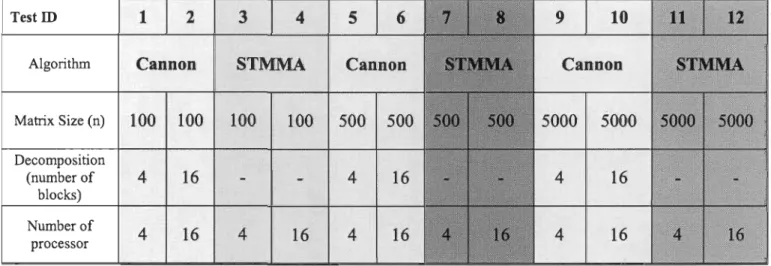
Table 4-1 Comparison between the perfonnance ofITPMMA (STMMA) and Cannon Aigorithms for matrices of 100x l00, 500 x500, and 5000x5000 ... 57

Table 4-2 Different sizes of matrices with 16 processors in parallel, where the matrices size is multiplicand of the number of processors ... 63

Table 4-3 multiplying different sizes ofmatrices on 16 processors, where the matrices size is not multiplicand of the number of processors (balanced load will be clear with ITPMMA algorithm) ... 66

Table 4-4 comparison between different size matrices multiplication, where the size of the matrices are multiple and non-multiple of the processors ... 68

Table 4-5 Non-square matrices -750 x 700 - with different number of processors ... 69

Table 4-6 Fixed size of matrices with different number of processors, where the matrices size is multiple of the number of processors ... 72

(13)

Table 5-1 Parallel Laplace's Equation Solution using Gauss-Seidel Iterative

method on 2D ... 81

Table 5-2 Parallel Laplace's Equation Solution using Gauss-Seidel Iterative method on ClusteredlD ... 84

Table 5-3 Speed up and efficiency of parallel gauss-seidel iterative solution of Laplace's equation in Decomposition 2D, for 128 processers, for very large matrices sizes ... 88

Table 5-4 Speed up and efficiency of parallel gauss-seidel iterative solution of Laplace' s equation in Clustered 1 D, for 128 processers, for very large matrices sizes ... 88

Table 5-5 Speed up comparison for clustered ID vs Decomposition 2D for parallel gauss-seidel iterative solution of Laplace' s equation in, for 128 processers, at very large matrices size ... 89

Table C-O-l PUMMA (MBD2), [119] ... : ... 124

Table C-0-2 SUMMA, [120] ... 124

(14)

List of Figures

Figure 2-1 Matrix Multiplication problem as benchmark problem for Intel

processor performance [39] ... 12

Figure 2-2 Systolic Aigorithm ... 18

Figure 2-3 Layout of the A and B matrices in the systolic matrix-matrix multiplication algorithm for A4x4xB4x4 task mesh. The arrows show the direction of data movement during execution of the systolic algorithm. [55] ... 19

Figure 2-4 Cannon's algorithm layout for n = 3 ... 20

Figure 3-1, SeriaI Matrix Multiplication ... : ... 27

Figure 3-2 Simulation of pre ITPMMA Aigorithms ... 28

Figure 3-3 Simulation of ITPMMA Aigorithm ... 28

Figure 3-4 ITPMMA Aigorithm flowchart ... 30

Figure 3-5 Task distribution of A4x4 x B4x4, where each processor will produce part of the result matrix C4x4 ... 33

Figure 3-6: Pseudo code executed by processor PO ... 34

Figure 3-7: Pseudo code executed by processor Pl ... 34

Figure 3-8: Pseudo code executed by processor P2 ... 34

Figure 3-9: Pseudo code executed by processor P3 ... 35

Figure 3-10 Task distribution of A12x12 x B12x12, where each processor will produce part of the result matrix C12x12 ... 36

Figure 3-11: Pseudo code executed by processor PO, to produce the frrst and the fifth and the ninth columns of the result matrix C 12x12 ... 37

Figure 3-12: A12x12 x B12x12 using ITPMMA algorithm for parallel matrix multiplication ... 38

(15)

Figure 3-13 Tasks to be performed by each processor of the eight processor to

produce the matrix C12x12 ... 40 Figure 3-14 Task distribution of A12x12 x B12x16, where each processor will

produce different part of the result matrix C12x16 ... 42

Figure 3-15 Multiplions of matrices A(3 x 3)

*

B(3 x 5) = C(3 x 5) using 3

processors ... 43 Figure 3-16 Task distribution of A12x12 x B12xlS, where each processor will

produce part of the result matrix C12xlS ... 44

Figure 4-1 Speed up oflTPMMA compared with Cannon ... 59

Figure 4-2: Speed up comparison for 4 processors between ITPMMA Cannon

algorithms ... 60

Figure 4-3: Speed up comparison for 16 processors between ITPMMA Cannon

algorithms ... 60

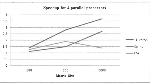
Figure 4-4 ITPMMA Aigorithm Speed up against both Cannon Aigorithm, and Fox Aigorithm where the matrices size is multiplicand of the

number of processors ... 63

Figure 4-5 Speed up of ITPMMA algorithm against both Cannon Aigorithm, and Fox Aigorithm where the matrices size is not multiple of the

number ofprocessors ... 67

Figure 4-6 Matrices multiplication of size multiple and non-multiple of the

processors in use ... 69 Figure 4-7 Parallel Processing Time ITPMMA algorithm against both Cannon

Aigorithm, and Fox Algorithm where the matrices size of

750x700 is not multiple of the number ofprocessors ... 70

Figure 4-8 Parallel Processing Time for matrices multiplication of two different sizes 750x700, and 1024xl024. A: ITPMMA algorithm, B:

Cannon Algorithm, C: Fox Aigorithm ... 71

Figure 4-9 Parallel Processing Time for ITPMMA algorithm against both Cannon Aigorithm, and Fox Aigorithm where the matrices size is multiple of the number of processors for matrices of

1024xl024 ... 73

Figure 4-10 Execution time per processor for ITPMMA, Cannon, and Fox

(16)

Figure 5-1 Laplace Equation problem presentation, reds are boundary points

while blue are interior points ... 79

Figure 5-2 ID Decomposition ... 79

Figure 5-3 2D Decomposition ... 80

Figure 5-4 Data dependency of2D Decomposition ... 80

Figure 5-5 ID decomposition technique, total time units is 196 units ... 81

Figure 5-6 2D decomposition technique, total time units is 147 units ... 82

Figure 5-7 Clustered ID decomposition technique, total time units is 73 units ... 83

Figure 5-8 Clustered ID decomposition processors utilization ... 83

Figure 5-9 Speed up and efficiency ofparallel gauss-seidel iterative solution of Laplace' s equation in 2 dimentions ... 85

Figure 5-10 Speed up and efficiency ofparallel gauss-seidel iterative solution of Laplace's equation in clustered 1 dimensional decomposition ... 86

Figure 5-11 Speed up of parallel gauss-seidel iterative solution of Laplace' s equation in both data decomposition techniques at 4 processors ... 86

Figure 5-12 Speed up ofparallel gauss-seidel iterative solution of Laplace's equation in both data decomposition techniques at 16 processors ... 86

Figure 5-13 Speed up and efficiency of parallel gauss-seidel iterative solution of Laplace's equation in clustered ID vs Decomposition 2D, for four processers ... 87

Figure 5-14 Speed up and efficiency of paraUel gauss-seidel iterative solution of Laplace's equation in clustered ID vs Decomposition 2D, for sixteen processers ... 87

Figure B-0-1 matrix-point of-view and processor point-of-view for PUMMA, SUMMA, andDIMMA ... 107

Figure B-0-2 PUMMA Single Data Broadcasting ... 108

Figure B-0-3 PUMMA Multiple Data Broadcasting 1 ... 109

Figure B-O-4 PUMMA Multiple Data Broadcasting 2 ... 110

Figure B-0-5 SUMMA algorithm ... 111

(17)

Figure B-0-7 DIMMA Aigorithm ... 114

Figure B-0-8 Coppersmith and Winograd 2010 (1/2) [13] ... 118

(18)

List of Symbols

f = number of arithmetic operations units

tr= time per arithmetic operation«

te

(time for communication) c = number of communication units

q = f / c average number of flops per communication access.

nproc = number of processors nblock = number ofblocks

(19)

The need for vast computing power in so many fields like forecasting the weather, analyzing DNA material, simulating earthquakes etc. has led for looking for paraUel and distributed computing, in the light. of the limited speed of the classic computers and processing power due to the physical constraints preventing frequency scaling. On the other hand, the physicallimits been achieved at the hardware level in processors industry, which leads for opening the do ors to design paraUel processors in the mid of 1980's by introducing the paraUel processing and networks of computers [1-8]. By the 1990's, the Single Instruction Multiple Data (SIMD) technology show up, and later multi-core platforms in the mainstream industry such as multi-core general purpose architectures (CPUs) and Graphics Processing Units (GPUs) where several cores working in paraUel inside the processor chip [4, 9, 10- 12]. New processors show vast computing power [4, 6, 13-15]. Multi-core i7 CPU is the most updated paraUel CPU produced by Intel at PC level; While latest NVidia Graphics Processing Unit has 1536 core at its VGA card Tesla KI0, which has two GPUs, which implies 1536 x 2 = 3,072 processors running in paraUel [16], which is needed for applications of seismic, image, signal processing, video analytics. This implies that the future software development must support multi-core processors, which is paraUel processing.

(20)

Parallel processing has opened an era to have super computing power at the cost of several PCS. 80, connecting several PCs into a grid could be utilized as one single supercomputer by the help of certain algorithm to manage the distributing of the load among the active connected PCS. Well, parallel processing did not stop here, but parallel processing extends to inc1ude computers and super computers connected over internet, where the load could be distributed over connected super computers to have enormous parallei processing power. AU paraUel algorithms until the moment depended in decomposing the data of a problem

into blocks and perform the functionality on it, in parallel mode taking in consideration the data and the functional dependency among the data.

Data Decomposition in general having two modes, one dimension (ID), where the data will be set of strips, where each processor will process one single strip at a time; and the other mode is two dimensions decomposing (2D), where the data will be set ofblocks, and each processor will process single block at a time.

In addition, existing parallel algorithms did not address and utilize the parallei capabilities of the new processors, like multicore and other enhancement like cache memory and wide address bus of 64 bit. AlI paraUel algorithms have kept looking at the processor on the old architecture design. For example, they are considering the grain applications, where the application will be divided into the most simple functions, so each processor will process these simple functions and getting the next afterword; while aU these algorithms are not looking at high capabilities of the new processors, where it can process more than a function at a time, dual core processors processes two functions a time, while Intel Xeon Phi processor has 61 cores, which implies it processes 61 functions at a time. Existing parallei algorithms sends one single function to each processor regardless number of cores

(21)

it has. In addition, the new processors architecture has different levels of cache memory which allows for more data upload capacity to reduce the access time of RAM, so cache memory leads to faster processing for complex functions which need huge chunk of data; Existing parallel algorithms do not consider the availability of cache memory and keep send simple math functions to each processor, which is a bad exploitation of modem architecture processors.

In this thesis, new technique for parallel processmg will be introduced, which will overcome the drawbacks of the previous algorithms. The technique is called ITPMMA algorithm, it depends on dividing the problem into set of tasks, which implies the data will not be decomposed in ITPMMA algorithm, and instead the problem will be decomposed into independent sets of operations, where each processor will execute independent operations and will upload what data it needs. In addition, ITPMMA algorithm will utilize the capabilities of the parallel and multi-core processors, which is absent in the existing parallel algorithms.

1.1. Motivation

Numerical problems consume a lot of processing resources which leads to utilize the parallel processing architecture. Since 1969, parallel algorithms start showing up, [17-21]. Parallel Matrix Multiplication algorithms were one of the earliest parallel processing algorithms that appeared since then. So, since 1969 for homogenous clusters like Systolic algorithm [22], Cannon's algorithm [23], Fox and Otto's algorithm [24], PUMMA (parallel Univers al Matrix Multiplication) [25], SUMMA (Scalable Universal Matrix Multiplication) [26] and DIMMA (Distribution Independent Matrix Multiplication) [27]. Ali these algorithms had been designed for distributed memory platforms, and most of them use the

(22)

popular ScaLAP ACK library [28, 29], which inc1udes a highly-tuned, very efficient routine targeted to two-dimensional ptocessor grids.

PUMMA algorithm maximizes the reuse of the data that have been hold in the upper levels of the memory hierarchy (registers, cache, and lor local memory) [16]. PUMMA, which

had been developed in 1994, did not address the time consumption by exchanging intermediate results between processors.

SUMMA algorithm, been developed in 1997. It has introduced the pipelining in PUMMA to maximize reuse of data. In addition, SUMMA reformulated the blocking method in terms of matrix-matrix multiplications instead of matrix-vector multiplications, which reduced the communication overhead [26]. In general, SUMMA did not address the time consumption of the communication between processors. In addition, SUMMA did not address the cache memory of the modem processors.

On the same year, 1997, Choi [27] has developed DIMMA algorithm. "The algorithm introduced two new ideas: modified pipelined communication scheme to overlap computation and communication effectively; and to exploit the least common multiple (LCM) block concept to obtain the maximum performance of the sequential BLAS - Basic Linear Algebra Subprograms - routine in each processor" [27]. But still, DIMMA did not,

address the huge time consumed on communication between processors to exchange the intermediate results.

In 2005, NGUYEN et al. [29] combined the use of Fast Multipole Method (FMM) algorithms and the parallel matrix multiplication algorithms, which gave remarkable results. Nevertheless, the algorithm still suffers data dependency and high communication

(23)

cost among the processors. Moreover, the algorithm does not address heterogeneous environments.

In 2006, Pedram et al. [30], have developed high-performance parallel hardware engine for matrix power, matrix multiplication, and matrix inversion, based on distributed memory. They have used Block-Striped Decomposition (BSD) algorithm directly to implement the algorithm. There was obvious drawback related to processors' speed up efficiency. The algorithm reduces memory bandwidth by taking advantage of reuse data, which results in an increase in data dependencies.

On 2008 James Demmel developed a new algorithm to minimize the gap between computation and communication speed, which continues to widen [31]. The performance of sparse iterative solvers was the aim of this algorithm, where it produced speedup of over three times of seriaI algorithm. In fact, the increasing gap between computation and communication speed, is one of the main points to be addressed by reducing the communication between processors as much as possible. The algorithm still suffers data dependency and communication; especially for large matrices sizes.

In 2008 Cai and Wei [32] developed new matrix mapping scheme to multiply two vectors, a vector and a matrix, and two matrices which can only be applied to optical transpose interconnection system (OTIS-Mesh), not to general OTIS architecture, to reduce communication time. They have achieved sorne improvements compared to Cannon algorithm, but it was expensive in term of hardware cost. In addition, the algorithm did not add any new value in term of algorithm design.

(24)

In 2009, Sotiropoulos and Papaefstathiou implement BSD algorithm using FPGA device [33]. There was no achievement in terms of reducing data dependencies and communication co st.

In 2012, Nathalie Revol and Philippe Théveny developed new algorithm, called "Parallel Implementation of Interval Matrix Multiplication" to address the implementation of the product of two dense matrices on multicore architectures [34]. The algorithm produced accurate results but it fails to utilize the new features of the multicore architectures processors, as it has targeted in advance.

In 2013 Jian-Hua Zheng [35] proposed new technique based in data reuse. It suffers from a lot of data dependency and high communication cost.

In 2014, another decomposition technique called Square-Corner instead of Block Rectangle partition shapes to reduce the communication time has been proposed in [36]. The research was limited to only three heterogeneous processors. For sorne cases, they have reported less communication time and therefore showed a performance improvement.

AIso, in 2014 Khalid Hasanov [37] introduced hierarchy communication scheme to reduce the communication co st to SUMMA algorithm. Although achieved sorne better performance, pre ITPMMA algorithm drawbacks like data dependency and communication cost are still there. Moreover, this algorithm is for homogenous environment.

Other algorithms have been designed later on to enhance the . process of matrix multiplication and to reduce the processing time. In 2014, Tania Malik et al. [38] proposed new network topology to decrease communication time among the processors. The algorithm suffers from more data dependencies between the processors. The major

(25)

drawback of aIl prevlOus parallel algorithms developed until now need homogenous processor architecture, and never addressed heterogeneous processors, except NGUYEN et al. [29], which conclude very negative results, so, by executing these algorithms in a grid of several PCs - heterogeneous environment - would have a lot of incompatible latency factors.

Having homogenous environment, aIl parallei algorithms, either for parallel matrix multiplication as we will see in this thesis, or for any numerical problem else, all existing algorithms suffer from classic drawbacks, like:

1. The optimal size of the block ofthe decomposed matrices.

2. The communication time of the exchanged messages among the processors, which is proportional to number of processors and number of the blocks of the decomposed matrices.

3. Data and functional dependency between the processors. 4. Poor load balance especially with non-square matrices.

1.2. Originality

In this thesis, a new novel framework for parallel processing has been developed to add the following new values:

1. Reducing the communication time among the parallel processors to ZERO.

2. No processor becomes idle or in ho Id, waiting other processors output until the parallei operations over.

(26)

1.3. Objectives

Thesis objectives to develop a novel framework for parallel processing which implies reconstruct the parallel problem into independent tasks to:

1. Reduce the idle time of the processors to increase the efficiency, and this to be

achieved by:

a. Proper load balance among the processors.

b. Utilizing the modem processor architecture capabilities in term of multicore and cache memories of different levels.

2. Reduce the communication time among the processors, by eliminating the data dependencies by reconstructing the parallel problem into set of independent tasks, to reduce the communication time among processors to zero.

On the other hand, for numerical problems where reconstructing the parallel problem into independent tasks is not within hands, like solving Laplace equation in parallel, a new data decomposing technique is developed, to reduce the communication time among the processors, and reduce idle time of the processors, to increase the efficiency.

1.4. Methodology

To satisfy the objectives ofthis thesis, 1 am to follow the procedure below:

1. Review literature of parallel matrix multiplication and data decomposition techniques.

2. Study in details different parallel algorithms and data decomposition techniques to find out its drawbacks.

(27)

3. Develop common diagram to setup new framework for parallel processing to address the drawbacks of the previous algorithms.

4. Develop new parallel matrix multiplication algorithm and new data decomposition technique within the new framework.

5. Test the new framework on small environment of 4 and 16 processors.

6. Test the new framework on the advanced supercomputer CLUMEQ.

7. Compare the results of the performance of the new framework with benchmark algorithms like Cannon algorithm and Fox algorithm.

1.5. Thesis Organization

This thesis is organized into six chapters. Chapter 1 is an introduction for the thesis to show the motivation, originality, objectives of the research and the methodology.

Chapter II, titled "Matrix Multiplication", 1 will discuss the common Parallel Matrix Multiplication Aigorithms in terms of performance, which incIudes speed up, time complexity, load balancing, data dependencies.

Chapter III, titled "ITPMMA algorithm for Parallel Matrix Multiplication (STMMA)",

presents the proposed algorithm followed by the results and comparisons with parallel matrix multiplication algorithms.

Chapter IV, titled "Analysis and Results", presents the experimental results which showed that the ITPMMA algorithm achieved significant runtime performance on CLUMEQ supercomputer and also a considerable performance compared by other algorithms like

(28)

Cannon Algorithm and Fox Algorithm. In these experiments 1 have used up to 128 processors in parallel, and about 40000 matrices size.

Chapter V, titled "The clustered 1 Dimension decomposition technique" presents the new data decomposition technique, developing paralle1 solution for Laplace equation using Gauss-Seidel iterative method, and test the results and compare it with same of 1 dimension and 2 dimensions data decomposition techniques.

Finally, Chapter VI presents the conclusion and explores the opportunities for the future that build upon the work presented in this dissertation.

(29)

Chapter 2 - Matrix Multiplication

2.1.Introduction

In this chapter 1 will address the matrix multiplication problem in seriaI and parallel mode. This problem will be used to describe the efficiency of the parallel algorithms; in fact,

matrix multiplication has been used as benchmark problem for parallel processing algorithms for several reasons:

1. It is easily scaled problem for a wide range of performance; its size grows like N3 for matrices of order N.

2. It has two nested loops plus the outer loop, total of three loops; the most inner loop consists at least a single multiply and add operation. Where the loops can be parallelized or to achieve high performance.

3. Computation independency, where the calculation of each element in the result matrix is independent of all the other elements.

4. Data independence, where the number and type of operations to be carried out are independent of the data type of the multiplied matrices.

5. Different data types like short and long integers and short and long floating-point precision can be used, which promises for different levels of tests. Aiso it allows for utilizing of the capabilities of the new processors, which has high cache memories, by

(30)

multiplying long type matrices, which needs high SlZe of cache memory for intermediate results.

6. Number offloating point operations (flops) easily is calculated.

7. Matrix multiplication is used as bench mark problem to test the performance of so many processors, like Intel, as shown in the figure 2-1, below.

Higher ig Better 1.5 QI U !: 1.25 lU 1 E li.. o 't QJ 0.75 Q.

.

_...

~

lU Qi ~ 0.5 . Matrix Mu[tipUcat'ion LINPACK* MKl Il.0.5 1.36 '

. Intel® Xeon® Proœsoor E5-2697 v2 (3or-t Cache, 2JO GHz)

!

.

Inte!® Xeon® Proœssor E5-2687W v2 (2Srlll: Cache, 3.40 GHz)

• Intel® Xeon® Proœsoor E5-2687W (20M Cache, 3.10 GHz, S.OO GTJs Intel® QPl)

Figure 2-1 Matrix Multiplication problem as benchmark problem for Intel processor performance [39].

In this chapter, sorne important aspects of matrix multiplication will be addressed, together with the outstanding characteristics of the already developed parallelization algorithms, like cannon and fox algorithms.

(31)

2.2. Matrix Multiplication Definition

It is defined between two matrices only if the number of columns of the first matrix is the same as the number of rows of the second matrix. If A is an i-by-k matrix and B is a k-by-j matrix, then their product AB is an i-by-j matrix, is denoted by Cij=Aik x Bkj, which be given by

c··

U =

In

A'~ k X Bk' J k=l

Eq.21

And it is calculated like

So,

Eq.2-3

Which is different than BA, which is denoted by Dij= Bkj x Aik, given by

=

In

Bk' _.}xA_1.'_k

k=l

Eq.2-4

So,

Eq.2-5

Which implies matrix multiplication is not commutative; that is, AB is not equal to BA. The complexity of matrix multiplication, if carried out naively, is O(N3), where N is the size of

(32)

product matrix C. So for the Matrix multiplication of 4x4 size, the complexity is O(~) =

0(43)= 64 operations, or the timing of 64 operations.

In 1969, Volker Strassen has developed Strassen's algorithm, has used mapping of bilinear combinations to reduce complexity to 0(n1081₍₇₎ _{(approximately}_0(n2

.807 ..

».

The algorithm is

limited to square matrix multiplication which is considered as a main drawback.

ln 1990, another matrix multiplication algorithm developed by Don Coppersmith and S. Winograd. The algorithm has complexity of 0(n2.3755). [40]

In 2010, Andrew Stothers gave an improvement to the algorithm, 0(n2.3736) [41]. In 2011, Virginia Williams combined a mathematical short-cut from Stothers' paper with her own insights and automated optimization on computers, improving the bound to 0(n2.3727) [42].

2.3. Seriai Matrix Multiplication Algorithm

2.3.1. SeriaI Algorithm

The seriaI algorithm for multiplying two matrices is taking the form: for (i = 0; i < n; i++) for (j = 0; i < n; j ++) c[i][j] = 0; for (k = 0; k < n; k++) c[i][j] += a[i] [k]

_*

b[k] [j] end for end for end for

(33)

2.3.2. Strassen 's algorithm

In 1969, Prof essor

v.

Strassen [36] developed new algorithm known by his name, Strassen's algorithm, where the complexity ofhis algorithm is 0(Nl097jl092) = 0(NL092 7)

= 0(N1n7), which will be equal to 0(4L0927) = 14.84, which is less than 64, i.e. to multiply

two 4x4 matrices using Strassen's algorithm, the algorithm needs the time of 14.84

operations, rather than the time of 64 operations using the standard algorithm .

To simplify Strassen's algorithm, 1 will implement it on the following matrices

multiplications:

So, we ron the below 7 quantities:

Pl = (AI2 - A22) x (B21

+

B22)

P2 = (An

+

A22) x (Bn

+

B22)

P3 = (AlI - A2I) x (BII

+

BI2)

P4 = (AlI + A12) x B22

Ps= AlI x (B12 - B22)

P6 = A22 x (B21 - Bn)

(34)

And produce the product matrix C, we run the below summations

The main drawback of Strassen's algorithm is the size product matrix should be product of 2, i.e. 21, 22, 23, 24, 25, ... , so for matrices multiplication of size 5, where 22 < 5 < 23, we

need to pad the matrices by zeros, till we have 8x8 matrices and multiply them. Recent studies study the arbitrary size of the multiplied matrices by Strassen algorithm in more details [43] but without getting better performance. So for Strassen's algorithm for matrices multiplication of size 3x_3,_{we have 7 multiplies and 18 adds. The complexity of}_the algorithm for matrices multiplication of size nXn can be computed as 7*T(n/2)

+

18*(n/2)2

= 0(NL092 7)= 0(8L0927)= 0(2310927)= 0(2l0927)3 = 73; while if we use standard matrices

multiplication, the complexity is 0(53) = 53 = 125 which is less than 73= 343, which is 2.744 times the complexity of Strassen's algorithm. And the difference become so huge when we have big matrix size, let us say a matrices multiplication ofsize 127x_I27,_{and 127} is not multiplicand of 2, the nearest multiple of 2 is 128, so, 128x128 matrices multiplication, we do have complexity of O(128L0927)= 0(2710927)= O(2l0927)7 = 77= 823,543; while if we go for the standard matrices multiplication where the complexity is 0(N3)

=

0(1273)

=

2,048,383; which is 2.49 times the complexity of Strassen's algorithm, so Strassen's algorithm has positive effect. While ifwe consider matrices multiplication of

(35)

slze 70x_{70, agam, we need to pad it with zeros till we reach} 128x 128 matrices

multiplication, where the complexity of standard multiplication is 0(JV'3)

=

0(703)

=

343,000, so, the complexity of Strassen's algorithm is 2.4 times the complexity of standard multiplication, so Strassen's algorithm has negative effect.

It is clear that the evaluations of intermediate values Pl, P2, P3, P4, Ps, P6, and P7 are independent and hence, can be computed in parallel.

Another drawback of Strassen's algorithm is the communication between the processors [44, 45, and 46]. Sorne other researches [47] focus on optimizing the communication between processors at the execution of Strassen's algorithm, where they could obtain sorne success at different ranges according to the size of the matrices and number of processors; but they could not eliminate the communication among the processors to zero.

On the other hand, many researches have tried to extract parallelism from Strassen's algorithm, and standard matrices multiplication algorithm [48], and many researches have tried to extract the algorithm on multi-core CPUs [49, 50, and 51] to exploit more performance. In 2007, Paolo D'Alberto, Alexandru Nicolau [52] have tried to exploit Strassen's full potential across different new processors' architectures, and they could achieve sorne success for sorne cases, but still, they have to work with homogenous processors. While in 2009, Paolo D'Alberto, Alexandru Nicolau have developed adaptive recursive Strassen-Winograd's matrix multiplication (MM) that uses automatically tuned linear algebra software [53], to achieve up to 22% execution-time reduction for a single core system and up to 19% for a two dual-core processor system.

(36)

2.4. Parallel Matrix Multiplication Algorithms

Parallel algorithms of matrices multiplication are parallelization of the standard matrices multiplication method.

2.4.1. Systolic Algorithm

One of the old parallel algorithms returns to 1970, but still active algorithm till moments [54]. It is limited to square matrix multiplication only. In this algorithm, matrices A, B are

decomposed into submatrices of size

.JP

X

.JP

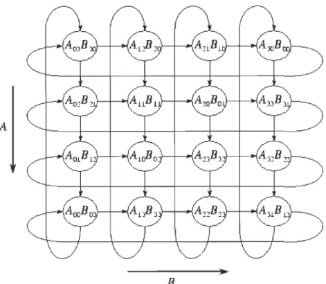
each, where P is number of processors. The basic idea of this algorithm is the data exchange and communication occurs between the nearest-neighbors.

MatrixA MatrixB

A(l,ll AI1,l} Atl,3 A(lA) B(l,l) B(1,2) B(1,3) B{VI

A(2,l) A(2,2) A(2,3) A(1,4) B(2,l) B(2,2) B(2,3) B(2,4)

A(3,l) A(3,2) A(3,3) A(3A) B(3,l) B(3,2) B(3,3) B(3,4)

A(4,l) A(4,2} A(4,3) A(4A) 8(4,1) B(4,2) B(4,3) BIII,4)

C(1,11=Atl,l)4B{1,4J+A(1,2)"B(1.4)+A(1,3)"B('!,4)+A(1,4)"B{4,4!

(37)

A

n

Figure 2-3 Layout of the A and B matrices in the systolic matrix-matrix multiplication algorithm for A4x4xB4x4 task mesh. The arrows show the direction of data movement during execution of the systolic algorithm. [55]

Table 2-1 The performance of the algorithm being studied by [33]

Task Transpose B matrix

Send A, B matrices to the processors Multiply the clements of A and B Switch processors' B sub-matrix Gcnerate the resulting matrix Total execution time

2.4.2. Cannon Algorithm 2n2 tf 2m2p te

m2n

tf n2 te n2 tf+ n2 'te Execution time tc(m2 _n

₊

_3n2 )

+

tc(4n2 )

It is a memory efficient if the multiplied matrices are square. The blocks of matrix A to rotate vertically while matrix B blocks to rotate horizontally, this can be handled using circular shifts to generate the product matrix C. In fact, it replaces the traditionalloop

(38)

With the loop

..fP-l

C- . l,} = "

L

A· l, k X Bk' .}

k=O

..fP-l

Ci,j =

L

AW+ j+k)mod..fP X B (i+ j+k)mod..fP,j

k=O

The Pseudo-code for the Cannon Matrix multiplication algorithm

% P number of processors % s size of the matrix

For i = 0 to P - 1

A(i, j)=A(i,(i+j) mod p %left-circular-shift row i of A by i shifts (skew of A)

For j = 0 to P -1

B(i, j)=B((i+j) mod p, j) %up-circular-shift row j ofB by j shifts (skew ofB)

For (i = 0 to p-l) and (j = 0 to p-l) C(ij) = C(ij) + L~=l A(i, k)

*

BCk, j)

A(i, j)=A(I,(i-j) mod p % lefl-circular-shifl each row of A by 1

B(i, j)=B«i-j) mod p, j) % up-circ1.l1ar-shift each columll of B by 1

A, B initially A, B after skewing A, B after shift k = 1 A, B after shift k = 2 C{2,31 = A(2,1)*8(1,3) + A(2,2rB{2,3)

..

A(2,3)"B(3,3)

(39)

1/ SkewA & N

for i = 0 to 8-1 Il s = sqrt (P)

left-circular-shift row i of A by i Il cost = s*(a + 1Il/pIP) for i = 0 to 8-1

up-circular-sbift column i ofB by i // cast = s*(n + Ill/pIP)

Il ,l .. lultiply and shift

for k = 0 to s-1

local-multiply

left-circular-shift each row of A by 1

up-circular-shift each column ofB by 1

Il cost = 1 *(1I/s)3 = 2*n3/p3/2

! / cost = a + Ill/pif)

I! cost = a + n2.p/fl

• Total Time = 2*n3/p + 4* s*a + 4*~*n2/s

• ParaUel Efficiency = 2*n3 1 (p * Total Time)

= 1/( 1

+

a

*

2*(s/n)3

+

~

*

2*(s/n) )

= 1/(1

+

O(sqrt(p)/n»

• Grows to 1 as nls

=

nlsqrt(p)

=

sqrt( data per processor) grows

• Better than ID layout, which had Efficiency = 1/(1

+

O(p/n»

Table 2-2 The performance ofthe algorithm being studied by [56]

Task

~hift

A.

B matrices * '"'

Send A, B matrices to the processors

Mumplytlie=êlemenis~of A"andB' ,. ~"'w.~ _ _ , Shift A, B matrices

Generate th~ resulting mairix

Total execution time

2.4.3. Fox and Otto's algorithm

4n2 tr 2n2 t.~ n2tr Execution time 2(mn te

+

2m2 n tf)

n

1

_tr+

_ù

2 _te _'" tr(5m2 _n

₊

_5n2 )

+

tc(2n2

+

2mn)

Fox's algorithm for multiplication organize C =A x B into submatrix on a P processors. The

(40)

row of the processes, run local computation and then shift array B for the next turn computation. The main disadvantages, it is applied only for square matrices.

This algorithm being written in general in HPJava, we still use Adlib.remap to broadcast submatrix, matmul is a subroutine for local matrix multiplication. Adlib.shift is used to shift

arra~,

and Adlib.copy copies data back after shift, it Can also be implemented as

nested over and for loops.

Group p=new Procs2(P,P); Range x=p.dim(O); Range y=p.dim(l); on(p) //input a, b here; z] ] ) ; mode; float [[#,#, ]] a float [[#,#, ]] b

new float [[x,y,B,B]]; new float [[x,y,B,B]]; float [[#,#, ]] c new float [[x,y,B,B]]; float [[#,#, , ]] temp = new float [[x,y,B,B]]; for (int k=O; k<p; k++) {

over(Location i=xl:) {

float [[,]] sub = new float [[B,B]];

IIBroadcast submatrix in 'a' ...

Adlib.remap(sub, a[[i, (i+k) %P, z, z]]); over(Location j=yl:) {

IILocal matrix multiplication

ma tmul (c [ [i, j, z, z]], sub 1 b [ [i 1 j 1 z,

}

//Cyclic shift lb' in 'yi dimension

Adlib.shift(tmp, b , 1, 0, 0); Il dst, src, shift, dim,

(41)

"Two efforts to implement Fox's algorithm on general 2-D grids have been made: Choi, Dongarra and Walker developed 'PUMMA' [50] for block cyclic data decompositions, and Huss-Lederman, Jacobson, Tsao and Zhang developed 'BiMMeR' for the virtual2-D toms wrap data layout"[57].

2.S.Conclusion

In this chapter 1 have addressed the use of matrix multiplication as benchmark and the defmition of matrix multiplication, seriaI algorithms and parallel algorithms.

Parallei algorithms for carrying out matrix multiplication in different architecture since 1969 had been studied and analyzed. Parallei algorithms for matrix multiplication have common mode, it is subdividing the matrices into small size matrices and distributing them among the processors to achieve faster running time.

We found out that although so many parallei matrix algorithms have been developed since Cannon Aigorithm and Fox algorithm four decades ago, aIl these algorithms - described in Appendix B - still use the same methodology and framework of Cannon and Fox algorithms in term of data decomposition and communication among the processors. On addition, aIl these algorithms could not achieve a distinguished performance against both Cannon and Fox algorithms, which keep both algorithms as bench mark algorithms in parallel matrix multiplication.

Finally, Identification of BLAS, and the development till considering multi-core architecture had been shown in Appendix A.

(42)

Chapter 3 - ITPMMA algorithm for Parallel Matrix

Multiplication (STMMA)

3.1.lntroduction

Several parallel matrix multiplication algorithms had been described and analyzed in the previous chapter. AlI parallei matrix multiplication algorithms based on decomposing the multiplied matrices into smaller size blocks of data~ the blocks will be mapped and distributed among the processors, so each processor run matrix multiplication on the assigned blocks; this will reduce the whole time of the matrix multiplication operation to less than the time needed to complete this operation by utilizing one processor. AlI existing parallei matrix multiplications algorithms suffer from four drawbacks:

1. To defme the optimal size of the block of the decomposed matrices, so the whole operation can be produced by the minimum time. For example, multiplying matrices of size 64x64 over 4 processors, should the block size be 4x4 or 8x8 or 16x16.

2. The number of exchanged messages between the processors are highly time consuming; it is proportional to the number of the processors. On the other hand, the time of forwarding the messages relays partly on the network structure.

3. Data dependency between the processors, where sorne processors will stay idle waiting an intermediate calculation results from other processors. Data dependency increases as number ofblocks/processors increases.

4. Sorne algorithms suffer from another drawback, which IS the load balance,

(43)

In this chapter, new paralle1 matrix multiplication algorithm will be introduced, to overcome the above four drawbacks, which returns in vast difference in the performance in terms of processing time and load balance. For example, for a matrices multiplication of 5000x5000, it consumes 2812 seconds using cannon algorithm, while only 712 seconds needed using the new algorithm, which implies 4 times faster. 1 have implemented the algorithm initially using Microsoft C++ ver. 6, with MPI Library. 1 have execute it at Processors Intel(R) Core(TM) i5 CPU 760 @2.80GHz 2.79 GHz, the installed memory (RAM) was 4.00 GB, System type: 64-bit Operating System, Windows 7 Professional. Later 1 have implemented the algorithm using CLUMEQ supercomputer, where 1 have used up to 128 processors in parallel.

1 will reference to the new algorithm by the name ITPMMA algorithm. The basic concepts of ITPMMA algorithm were published on "Sub Tasks Matrix Multiplication Aigorithm (STMMA)", [59].

3.2.ITPMMA algorithm for Parallel Matrix Multiplication (STMMA)

Unlike previous algorithms, ITPMMA Aigorithm for ParaUe1 Matrix Multiplication does not defme new data movement or circulation; instead, it generates independent seriaI tasks follows the seriaI matrix multiplications shown below:

l:forIII=Otos-1 { 2: for 1=0 to s-1 { 3: for K=O to s-1 {

4: CU = CU

+

AIK xBKJ } } }

ITPMMA A1gorithm decomposes the paralle1 matrix multiplication problem into several independent vector multiplication tasks, keeping the processing details of each independent task to the processors, which are multicore processors, so 1 am utilizing the modem

(44)

architecture processors' capabilites. ITPMMA Aigorithm has the advantage to utilize the up-to-date processor architecture features in tenus of multicores and cache memories. In

fact, ITPMMA Aigorithm defmes each independent task as set of instructions to produce one element of the result matrix. Each single set is fully independent of production of any other set, or independent task. Each single independent task is being processed by one· single processor. Once each processor has completed the independent task been assigned to it, and produced an element of the result matrix, it processes the next independent task, to produce the next element, and so on. ITPMMA Aigorithm implies:

1. Zero data dependences so better processors' utilization since no processor stays on hold, waits for other processors' output,

2. Zero data transfer among the processors of the cluster, so faster processmg. Communications in ITPMMA Aigorithm is limited to the time needed to send the independent tasks lists by the server node processor to different processors, and to the time needed to receive back alerts and results by the other processors to the server node processor.

In this context ITPMMA Aigorithm has advantages of efficient use of the processors' time. Figure 3-1 simulates the seriaI matrix multiplication using one single core processor. Figure 3-2 simulates the previous parallel algorithms. It is clear that both processors P2 and P3 are on hold, till processor Pl over and switch to idle status. On addition, processors P4 will not start processing till both P2 and P3 over. The efficiency of using the processors' time is so poor. Each processor computes for 4 units oftime and 3 units for communication, and been on hold or idle for 9 units of time. So the computing efficiency of each processor is 4/16 =25%. On the other hand, figure 3-3 simulates paraUel multiplication using new algorithm

(45)

which is called Independent Tasks Parallel Matrix Multiplication Aigorithm (ITPMMA). Instead of decompose the data among the processors; we distribute the independent tasks among the processors. 80, processor Pl should produce the frrst row of Matrix C shown in figure 2, while processor P2 should produce the second row of Matrix C, and processor P3 should produce the third row, finally processor P4 should produce the fourth row ofMatrix C. For that, we need only 4 units of time to accomplish the tasks, in addition, no communication among the processors, aIso, no time for assembling the results, only to deliver it. One of the major advances of ITPMMA algorithm is efficiency of using the processors, no processor gets on hold or idie. The efficiency of each processor is 4/5 = 90%. x I---+--+-+---l

=

MatrixA4x8 Matrix C 4x4 Matrix B 8x4

•

• Computation Time

(46)

r::'9!I.II!!!!!!!!!!!i.

"

M " '~\,v« ',:<1 ~

...

' ,,~

....

'

.",,';

x

=

,

.

, ... ", ~ ~ ~ ~, ..;: MatrixA4x8 Matrix C 4x4 Matrix B 8x4 Computation Time

Communication Time - among processors

Communication Time -assembling and delivering data

Figure 3-2 Simulation of pre ITPMMA Aigorithms

x

MatrixA4x8

Matrix B 8x4

---::--+--Time

.Computation Time

DCommunication Time - delivering data

=

Matrix C 4x4

(47)

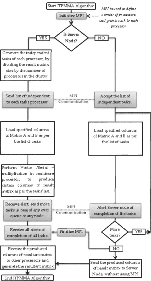
3.2.1. ITPMMAflowchart

ITPMMA Aigorithm for paraUel matrix multiplications, on the contrary of other parallel matrix multiplication algorithms, it depends on reformatting the matrix multiplication process into many independent vector multiplication operations, each vector multiplication operation will be carried out by single processor, to avoid any data dependency and processor-to-processor data transferring time. Figure 3-3 shows ITPMMA Aigorithm flowchart.

(48)

GenE!"al:e theindependent tas!< s of each processor, by di vi ding the result matrix

size by the numb er of

processors in the cluster

Load specified colurrms

of Matrtx A and B as per the list of tas!<s

ISE!"ial

multicor produc

of resul

Receive the produced col umns of resul tant mabix

MPlisused IDdifine numœr ifprocessors and gran ts rank ID each

processor

MPI

···~è~o·;;;;;;;J;Tê~·i:"i~;;;····

MI'I "'(:;I;;;~;;;:-i(:;li~;;;"

Load specified columns of Mabix A and B as p E!"

the list of tas!< s

to other processors and ... _ _ _ ... _-tSend the produced columns

general:ethe resultant matrix of result mabix to Server Node, without using MPI

(49)

ITPMMA Algorithm uses MPI library to defme the number of active processors on the c1uster and rank them. In addition, MPI library is used to transfer the lists of tasks to the processors and to forward task completion alerts from different processers to the node processor. So the server node: received bird sow

1. Defmes the processors available in the parallel c1uster and to rank them.

2. Generate the the independent tasks, so produce an element of the result matrix is considered as independent task.

3. Divides the last of independent tasks by the number of active processors in the c1uster. So for the output matrix of size 7000x7000 and number of processors is 128 active processors, (7000x7000)/128=382812.5, so 64 processors produce 382,812 independent tasks and 64 processors produce 382,813 independent tasks. So the time needed to process 7000x7000 matrix multiplication in paraIlel of 128 processors is equivalent process 620x620 in one processor.

4. Sends for each processor li st of independent tasks to be carried out.

5. Receives from each processor alert of completion when aIl assigned tasks have been carried out.

6. Redistributes the processor of any faulted processor(s) to other active ones by sending extra tasks for the high computing power processors, once the initial sent list of tasks of these processors had been carried out. Redistribution inc1udes shifting tasks from the over queued low computing power processors to the high computing ones; so this algorithm address the hetregenious enviroment.

(50)

MPI library will not be used to exchange any data at aIl, as aIl tasks are independent, so, no

processor receives any data from another processor to be able to complete its work, nor any

processor communicate with non-server node processor.

1 will explain the algorithm using different four examples:

1. Square Matrix multiplication, and the size of the result matrix is multiple of the

number of processors being used in parallel, like A4x4 x B4x4 = C4x4, for four

processors in parallel; weIl, the size of the result matrix is 4x4, is multiple of the

number ofprocessor in use, which is 4.

2. Square Matrix multiplication, and the size of the result matrix is not multiple of the

number of processors being used in parallel, A12x12 x B12x12 = C12x12, for eight

processors in parallel; it is obvious that 12 is not multiple of 8.

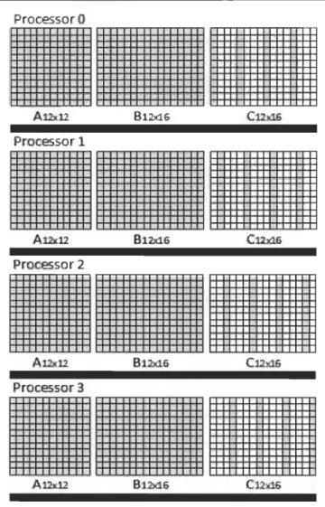
3. Non Square Matrix multiplication, and the size of result matrix is multiple of the

number of the processors being used in parallel, like A12x12 x B12x16 = C12x16, for four

processors in parallel; it is obvious that both 12 and 16 are multiple of 4.

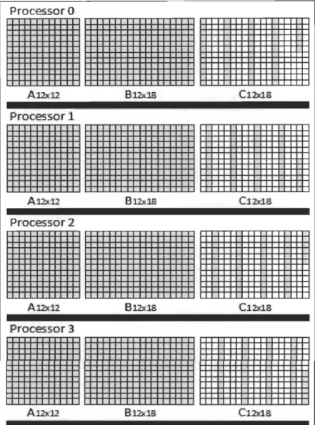
4. Non Square Matrix multiplication, and the size result matrix is not multiple of the

number of the processors being used in parallel, like A12x12 x B12x18 = C12xl8, for

four processors in parallel; it is obvious that 18 is not multiple of 4.

The second and the fourth example will help me to show how ITPMMA algorithm will

address the problem of load balance to be very obvious. On the other hand aIl previous

algorithms for parallel matrix multiplication are limited to square matrix multiplication

(51)

3.3.ITPMMA applied to different matrices sizes

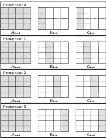
3.3.1. Square Matrix multiplication, size of the result matrix is multiple of the number of processors in paraUel

In this example, A4x4 x B4x4 being executed on four processors Po, Pl, P2, and P3, matrix A will be sent to aU processors, while one single column of matrix B will be sent to each matrix, so each processor produces part of the matrices multiplication result as shown of Figure. 3-4. Processo·rO

Ë

~x4; B.h* Cb4 Proces·so·rl

Ë

Ab ... B..:.. .. 1 Ct,,4; Proces.so·r2

Ë

Ab.4 B ... C4,,4 Proces·sor3

Ë

A .b4 ~".. C4",.4

Figure 3-5 Task distribution of A4x4 x B4x4, where each processor will produce part of the result matrix C4x4

Each processor processes separate independent tasks, so no messages of intermediate results will be exchanged, instead each processor produces what it needs when needed, that is to reduce the time consumed for exchange intermediate results between the processors

(52)

and to avoid data dependencie which put the processor on hold waiting results from other processors. So, Po will execute the code shown in Figure 3-5:

1 - far J=O ta 3{

2 - for K=O ta 3 {

3: CJO

+

AlK )( BK,]

4: }

5 - }

Figure 3-6: Pseudo code executed by processor PO

While Pl will execute the code shown in Figure 3-6:

1: for J-Q ta 3 { 2: for K=O ta 3 { ~. 3: CJl -

en

+

AlI< xBKJ 4: 5- } }

Figure 3-7: Pseudo code executed by processor Pl

While P2 will execute the code shown in Figure 3-7:

1 : for J=O ta 3 {

2; for KOta 3 {

3: CJ2 = CJ2

+

k K xBKJ

4: }

5: }

Figure 3-8: Pseudo code executed by processor P2

(53)

1: for J=O ta 3{ 2; for K=O ta 3 {

3:

4: }

5: }

Figure 3-9: Pseudo code executed by processor P3

As we can see, no processor waits its entries from another processor( s), and no processor sends sorne results to other processor, so we could reduce the data dependency and exchanged messages to zero, which has played backward role on the performance of the previous paraUe1 matrix multiplications. To generalize the case mentioned above, for

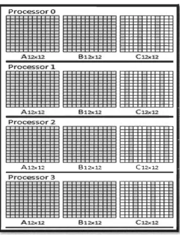
different matrices size, 1 will use the example of A12x12 x B12x12 = C12x12, for four paraUel processors. So, each processor will produce three columns of the matrix C, processor Po will produce three columns, these are the first and fifth and ninth columns of the matrix C12x12, Figure 3-9 shows task distribution of A12x12 x B12x12 = C12x12.

(54)

ProcessorO

. . .

Processor 1

. . .

B:12x:12 C:12x:12. Processor 2

. . .

Figure 3-10 Task distribution of AJ2x12 x B12x12, where each processor will produce part of the result matrix CJ2x12

Processor 0 executes the code shown in Figure 3-10, to produce the frrst and the fifth and the ninth columns of the result matrix C12x12.

(55)

1: for 3=0 to 11 { 2: for K=O to 11 { 3 : CJO - C,JO

+

AaR xBK,J 4 : } 5: } 1: for J=O ta 11 { 2: for K=O to 11 { 3: 4: } 5: } 1: for 3=0 ta 11 { 2: for K=O t o 11 { 3: CJS = CJ8

+

AaR xBRJ 4: } 5: }

Figure 3-11: Pseudo code executed by pro cess or PO, to pro duce the first and the fifth and the ninth columns of the result matrix Cl2xl2

While processor Pl produces different three columns, these are the second and sixth and tenth columns of the matrix C12x12, and so on for the remaining processors. Figure 3-11

shows the details of ITPMMA algorithm for the multiplication of A12x12 x B12x12, using four processors in parallel.

(56)

Matrix A12x12

The first processor wi Il

produce the first and fifth and ninth columnsof the

result matrix, that is

C[O][O]- C[ll][O], and

C[O][4] --->-C[1l][4], and C[O][8] --->-C[1l][8]

The second proc,essor

will produce the second

and sixth and tenth

columnsof the result matrix, that is C[O][l]-C[11][1], and C[O]{S] ----. C[11][5], and C[O][9]

--->-C[11][9]

The third processor will

produce the third and seventh and eleventh columnsof the result matrix, that is

C[O][2]-C[1l][2], and C[O][6] ----.

C[llJ[6], and C[O][lO] - C[ll][lO]

The fourth processor will

produce the fourth and eighth and twel:fth

co lumns of the result matrix, that is C[O][2]----. C[1l][2], and C[O][7]

-C[ll][7], and C[O][ll]

- C[ll][ll]

rvlatrix B 12x 12 Matrix Cl2><12

x

Result of the mst processor

Result of the .second processor

Result of the fourtIl processor

(57)

The tasks are fully independent tasks - so no processor needed to ex change data with other

processors - so there was no time being wasted by exchanging messages, and no processor

has stayed idle waiting its input from other processors, weIl, this is the essence of ITPMMA

algorithm.

3.3.2. Square Matrix multiplication, size of the result matrix is not multiple of the number of processors in paral/el

For this case, the size of the multiplied matrices is not multiple of the number of the

processor. In this example, we are to multiply A12x12 x B12x12, while the number of

processors is eight, where 12 is not multiple of 8. In this case, we have to overcome this

issue, and schedule the independent tasks between the processors equaIly, so the load is

balanced, and no processor will stay idle while other processors still overloaded. So, we can

run the schedule shown in Table 3-1, which satisfy the criteria of ITPMMA algorithm.

Table 3-1 Tasks to be performed by each processor

Processor erformed PO Pl P2 P3 P4 P5 P6 P7

Each processor produce 18 elements of the output matrix C, which satisfies the load

balance between the processors, also, each task - and so each processor - is independent

from any other tasks, and so, there is no exchanged messages. Figure 3-12 (A) shows the

time chart for the eight processors for this example A12x12 x B12x12 = C12x12 , it is obvious

that aIl processors working, and no processor is idle, and no processor finishes its tasks

(58)

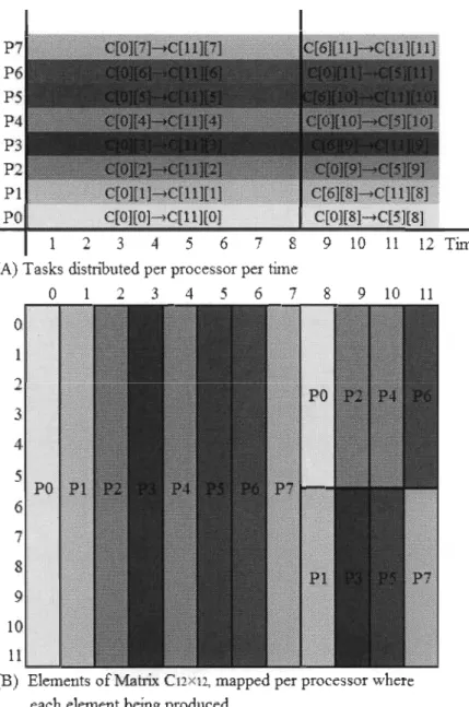
highest load balance been achieved. On the other hand, Figure 3-12 (B) shows the map of between the elements of the output matrix C12x12, and the processor that will pro duce each.

Finally, Figure 3-12 (C) shows the total number oftasks being produced by each processor.

(A) Tasks rustnbuted pet' processor per rime

o

l 2 3 4 5 6 7 8 9 10 Il

(B) Elements ofMatrix Cl2Xl1. mapped per processor where each element being produced

Total elements being

produced by a processor PO 18 Pl 18 P2 18 P3 18 P4 18 P5 18 P6 18 P7 18

(C) Toral tasks per each processor

Figure 3-13 Tasks to be performed by each processor of the eight processor to produce the matrix C12X12

Algorithme innovant pour le traitement parallèle basé sur l'indépendance des tâches et la décomposition des données

Université du Québec à Trois-Rivières

Service de la bibliothèque

Avertissement

L’auteur de ce mémoire ou de cette thèse a autorisé l’Université du Québec

à Trois-Rivières à diffuser, à des fins non lucratives, une copie de son

mémoire ou de sa thèse.

Cette diffusion n’entraîne pas une renonciation de la part de l’auteur à ses

droits de propriété intellectuelle, incluant le droit d’auteur, sur ce mémoire

ou cette thèse. Notamment, la reproduction ou la publication de la totalité

ou d’une partie importante de ce mémoire ou de cette thèse requiert son

autorisation.

PAR

Abstract

Foreword

Table of Contents

List of Tables

List of Figures

*

List of Symbols

te

Chapter 2 - Matrix Multiplication

.

...

~

!

.

c··

In

In

».

*

v.

+

+

+

+

+

=

=

=

=

.JP

.JP

n

m2n

+

+

L

L

*

..

+

*

+

*

+

=

=

+

A.

+

n

tr+

ù

+

+

+

arra~,

Chapter 3 - ITPMMA algorithm for Parallel Matrix

Multiplication (STMMA)

+

=

•

r::'9!I.II!!!!!!!!!!!i.

"

...

....

.",,';

=

_...

_*

₊

_tr+

_ù

₊