Performance Evaluation and Prediction of Parallel Applications

(1)

HAL Id: tel-00951125

https://tel.archives-ouvertes.fr/tel-00951125

Submitted on 24 Feb 2014

HAL is a multi-disciplinary open access

archive for the deposit and dissemination of sci-entific research documents, whether they are pub-lished or not. The documents may come from teaching and research institutions in France or abroad, or from public or private research centers.

L’archive ouverte pluridisciplinaire HAL, est destinée au dépôt et à la diffusion de documents scientifiques de niveau recherche, publiés ou non, émanant des établissements d’enseignement et de recherche français ou étrangers, des laboratoires publics ou privés.

Performance Evaluation and Prediction of Parallel

Applications

Georgios Markomanolis

To cite this version:

Georgios Markomanolis. Performance Evaluation and Prediction of Parallel Applications. Other [cs.OH]. Ecole normale supérieure de lyon - ENS LYON, 2014. English. �NNT : 2014ENSL0880�. �tel-00951125�

(2)

N◦ _{attribué par la bibliothèque : 2014ENSL0880}

École Normale Supérieure de Lyon

Laboratoire de l’Informatique du Parallélisme

THÈSE

en vue d’obtenir le grade de

Docteur

de l’Université de Lyon – École Normale Supérieure de Lyon

Spécialité : Informatique

au titre de l’École Doctorale Informatique et Mathématiques

présentée et soutenue publiquement le 20 Janvier 2014 par

Georgios Markomanolis

Performance Evaluation and Prediction of

Parallel Applications

Directeur de thèse : Frédéric Desprez

Co-encadrant de thèse : Frédéric Suter

Après avis de : Emmanuel JEANNOT

Jean-François Méhaut Devant la commission d’examen formée de :

Frédéric Desprez Membre

Emmanuel Jeannot Membre/Rapporteur

Jean-François Méhaut Membre/Rapporteur

Olivier Richard Membre

Frédéric Suter Membre

(3)

(4)

Abstract

Analyzing and understanding the performance behavior of parallel applications on various compute infrastructures is a long-standing concern in the High Performance Computing com-munity. When the targeted execution environments are not available, simulation is a reasonable approach to obtain objective performance indicators and explore various łwhat-if?ž scenarios. In this work we present a framework for the of-line simulation of MPI applications.

The main originality of our work with regard to the literature is to rely on time-independent execution traces. This allows for an extreme scalability as heterogeneous and distributed re-sources can be used to acquire a trace. We propose a format where for each event that occurs during the execution of an application we log the volume of instructions for a computation phase or the bytes and the type of a communication.

To acquire time-independent traces of the execution of MPI applications, we have to instru-ment them to log the required data. There exist many proőling tools which can instruinstru-ment an application. We propose a scoring system that corresponds to our framework speciőc re-quirements and evaluate the most well-known and open source proőling tools according to it. Furthermore we introduce an original tool called Minimal Instrumentation that was designed to fulőll the requirements of our framework. We study diferent instrumentation methods and we also investigate several acquisition strategies. We detail the tools that extract the time-independent traces from the instrumentation traces of some well-known proőling tools. Finally we evaluate the whole acquisition procedure and we present the acquisition of large scale in-stances.

We describe in detail the procedure to provide a realistic simulated platform őle to our trace replay tool taking under consideration the topology of the real platform and the calibration procedure with regard to the application that is going to be simulated. Moreover we present the implemented trace replay tools that we used during this work. We show that our simulator can predict the performance of some MPI benchmarks with less than 11% relative error between the real execution and simulation for the cases that there is no performance issue. Finally, we identify the reasons of the performance issues and we propose solutions.

(5)

(6)

Résumé

L’analyse et la compréhension du comportement d’applications parallèles sur des plates-formes de calcul variées est un problème récurent de la communauté du calcul scientiőque. Lorsque les environnements d’exécution ne sont pas disponibles, la simulation devient une approche raisonnable pour obtenir des indicateurs de performance objectifs et pour explorer plusieurs scénarios łwhat-if?ž. Dans cette thèse, nous présentons un environnement pour la simulation of-line d’applications écrites avec MPI.

La principale originalité de notre travail par rapport aux travaux précédents réside dans la déőnition de traces indépendantes du temps. Elles permettent d’obtenir une extensibilité maximale puisque des ressources hétérogènes et distribuées peuvent être utilisées pour obtenir une trace. Nous proposons un format dans lequel pour chaque événement qui apparaît durant l’exécution d’une application, nous récupérons les informations sur le volume d’instructions pour une phase de calcul ou le nombre d’octets et le type d’une communication.

Pour obtenir des traces indépendantes du temps lors de l’exécution d’applications MPI, nous devons les instrumenter pour récupérer les données requises. Il existe plusieurs out-ils d’instrumentation qui peuvent instrumenter une application. Nous proposons un système de notation qui correspond aux besoins de notre environnement et nous évaluons les outils d’instrumentation selon lui. De plus, nous introduisons un outil original appelé Minimal Instru-mentation qui a été conçu pour répondre au besoins de notre environnement. Nous étudions plusieurs méthodes d’instrumentation et plusieurs stratégies d’acquisition. Nous détaillons les outils qui extraient les traces indépendantes du temps à partir des traces d’instrumentations de quelques outils de proőling connus. Enőn nous évaluons la procédure d’acquisition complète et présentons l’acquisition d’instances à grande échelle.

Nous décrivons en détail la procédure pour fournir un őchier de plateforme simulée réaliste à notre outil d’exécution de traces qui prend en compte la topologie de la plateforme cible ainsi que la procédure de calibrage par rapport à l’application qui va être simulée. De plus, nous montrons que notre simulateur peut prédire les performances de certains benchmarks MPI avec moins de 11% d’erreur relative entre l’exécution réelle et la simulation pour les cas où il n’y a pas de problème de performance. Enőn, nous identiőons les causes de problèmes de performances et nous proposons des solutions pour y remédier.

(7)

Introduction

1.1 Motivation

Computational Science is the third scientiőc way to study problems arising in various domains such as physics, biology, or chemistry. It is complementary to theory and actual experiments and consists in conducting studies in silico. This approach makes an heavy use of resources located in computing centers. The eicient execution of a parallel application on a certain massively parallel hardware architecture demands the user to be familiar not only with domain-speciőc algorithms but also parallel data structures [1, 2]. It is not rare to observe situations where an application can not fully exploit a large number of processors in its execution, thus it does not scale well [3].Such cases can be caused by a not optimized application, the computer system or both. However, through performance evaluation a scientist can observe the performance of an application and can identify bottlenecks [4, 5, 6, 7, 8, 9]. The techniques which constitute the performance evaluation őeld can be classiőed into two categories: measurement and modeling techniques [10, 11, 12]. The latter is separated by many scientists into simulation and analytical modeling. A lot of approaches have been presented to evaluate the performance of an application. Some of them correlate the performance of an application with its scientiőc domain [13]. More precisely, in this approach the authors take data from three domains, the application’s working set, the hardware domain of the compute and network devices and the communication domain. The combination of visualizing and correlating these data, provides useful information about the behavior of the parallel application. On the other hand some researchers identify bottlenecks on a speciőc application which are related to the operating system such as noise, the cluster manager tool and őx them by applying some techniques to decrease the noise [14].

As the number of scientiőc domains producing results from in silico studies increases, the computing centers then have to upgrade their infrastructures in a continuous way. The resources impacted by such upgrades are of diferent kinds, e.g., computing, network and storage. More-over each kind of resource grows more complex with each generation. Processors have more and more cores, low latency and high bandwidth network solutions become mainstream and some disks now have access time close to that of memory.

The complexity of the decision process leading to the evolution of a computing center is then increasing. This process often relies on years of experience of system administrators and users. The former knows how complex systems work while the latter have expertise on the behavior of their applications. Nevertheless this process lacks of objective data about the performance

(9)

of a given candidate infrastructure. Such information can only be obtained once the resources have been bought and the applications can be tested. Any unforeseen behavior can then lead to large but vain expenses. This procedure could be completed with less risks by using simulation techniques. Simulation may help the dimensioning of compute clusters in large computing centers. Through simulations the scientists can understand the behavior of large-scale computers. Moreover it is possible to simulate an application for a platform that is not available yet to observe the performance and decide what would be the best hardware characteristics for the needs of the computer center.

Many universities do not provide large-scale computer systems to the researchers and stu-dents. Clusters are too expensive as also their maintenance. The access to another supercom-puters could cost also a signiőcant amount of money. In such cases the option to predict the performance of an application through simulation is really important. A scientist can execute simulations without using any resource and be able to validate or not his assumptions. Some times a multi-parameter application is needed to be executed, thus it would take a lot of time to try diferent parameters for each execution on a supercomputer. The students can study concepts of parallel computing without using a cluster but just their simulator. However, the performance evaluation and prediction are not always easy to be done.

1.2 Issues on Performance Prediction and Evaluation of

Parallel Applications

The őrst diicult step during the performance evaluation of a parallel application is the choose of the appropriate metrics. The metrics are essential for understanding the performance characteristics of applications on modern multicore microprocessor. They can indicate a relation between the performance bottleneck and the hardware. However, if a user is not familiar it can be a diicult task. A tool which can help the user was released by Texas Advanced Computing Center called PerfExpert [15] which basically executes an application four to őve times. During each execution the tool uses diferent metrics and it measures them periodically. As result it proposes which metrics represent any performance issue that occur mainly during the execu-tion of loops in the code. Moreover a tool called AutoScope [16] proposes code optimizaexecu-tion techniques based on the results from PerfExpert. However, performance measurement usually is not a harmonic task. Diferent parts of a code can cause non similar behaviors and diferent metrics could represent their performance. Computational science applications are constituted by iterative methods. A common method is to study the performance of each iteration [17, 18] where in some cases we can observe non similar performance between diferent iterations. The further analysis of the performance of an application should be achieved through extensive study of the measurements. The main issue with a őne grained measurement is the extra overhead caused by the instrumentation tool. When a user wants to correlate performance measurements with execution time, can not be sure what percentage of these measurements are caused by the instrumentation overhead. This makes the study harder and can hide some other phenomena or create artifacts that are not always easy to explain.

The increase of the hardware complexity raised the diiculty to predict the performance of an application. Diferent processors are constituted by diferent cache memory levels and size. The performance of an application can depend on the cache size. Moreover there are many types of networks, Ethernet Gigabit [19], Inőniband [20] etc. Each of them behave diferent and thus some analytical models should be created in order to simulate the applications. In this work we study Ethernet Gigabit networks. The studied parallel applications are based on the Message Passing Interface (MPI) [21]. The various implementations of the MPI, MPICH [22], and OpenMPI [23], can behave a bit diferent but always respecting the MPI standards. For

(10)

example some collective communications can behave similarly but not exactly the same. Thus the simulation of a parallel application is a diicult task where many aspects of the applications should be taken under consideration to predict correctly the performance.

1.3 Contributions

In this work we propose a new execution log format that is independent of time. This format includes volumes of computation (in number of instructions) and communications (in bytes) for each event instead of classical time-stamps. We present in detail an original approach that totally decouples the acquisition of the trace from its replay. Furthermore, several original scenarios are proposed that allow for the acquisition of large execution traces. These scenarios are only possible because of the chosen time-independent trace format and they can not be applied with other frameworks. We implement a new proőling tool based on our framework requirements which instruments exactly the necessary information from an application, it saves the measurement data directly into time-independent traces and it is more eicient than similar tools. We study the state of the art of the most well known and open sources proőling tools and we evaluate them with regard to our framework requirements. Moreover we justify which ones can be used for our work. We use various instrumentation methods and we evaluate them to show the evolution of the instrumentation overhead. As supporters of the open-science approach, we provide a step-by-step deőnition of an appliance to acquire execution traces on the Grid’5000 experimental infrastructure. Moreover we have our őles available in public to be used from other researchers. Some tools were implemented to extract the time-independent traces from well known proőling tools such as TAU, Score-P and gather them into a single node. We evaluate the time-independent trace acquisition framework to present the overhead, the advantages and disadvantages. The trace replay tool is built on top of a fast, scalable and validated simulation kernel. The implemented simulator tool is analyzed in detail and we describe how to use it by covering all the procedure from calibrating the simulator till the execution of a simulation. Finally, we predict through simulation the performance of some non adaptive MPI applications with small relative error between the real execution and simulation. In the cases that there are some performance issues, we investigate and őgure out what causes any performance issue.

1.4 Organization of the Document

The remaining of this document is organized as follows. Chapter 2 presents an introduction to some related topics. We present some benchmarks, we analyze some of them and we indicate which ones we use. Afterwards we present some techniques to evaluate the performance of an application such as the interface to access the hardware counters of the processors is introduced as also some instrumentation methods which are used to measure the performance of an application. We analyze the tracing, proőling, and statistical proőling methods and we explain the advantages and disadvantages.

In Chapter 3 we explore the time-independent trace acquisition framework. In the begin-ning we explain the motivation for this work, we introduce the time-independent trace format and we analyze the advantages. We provide more details about the whole framework and we mention the trace replay concept. There is an extensive analysis of the instrumentation of an application where we evaluate many well known tools with a score system which respects the framework requirements. We present our proőling library which can instrument an application with less instrumentation overhead and memory requirements. The instrumentation methods which we used are presented and compared. Moreover the acquisition of time-independent traces

(11)

is presented with all the execution modes that can be used and also instructions of how to re-produce the experiments on Grid’5000 platform. We have implemented some tools to extract time-independent traces from well known proőling tools such as TAU and Score-P as also gather them from all the participating nodes into a single node. Finally we evaluate the acquisition procedure to present the overheads of our framework.

Chapter 4 presents the time-independent trace replay. First of all the components of the simulation are introduced with the calibration procedure where is explained to the user how to calibrate the simulator. Afterwards the simulation backends that were used for the imple-mentation of the various versions of our simulator are presented with their diferences. At last we present the simulation accuracy of some MPI applications and we show that our framework predicts their performance.

(12)

Chapter 2

Background on Performance Evaluation

Chapter 1, analyzing and understanding the performance of a parallel application is a com-plex task. Some parallel applications may scale well when increasing the number of the processors while others may sufer from scalability issues. In general we could divide applications in two categories, those that fully exploit the performance of a computer system and to the ones that solve a real problem. Performance evaluation is usually performed thanks to various instrumen-tation methods when an application is executed on a real platform. However, there are two other approaches that provide insight about the behavior of an application: emulation and simulation. The purpose of this chapter is to introduce some basic concepts for the better understanding of the remaining of this document.

This Chapter is organized as follows. Section 2.1 presents some micro-benchmarks and benchmarks. We explain why they are used and how useful where for our case. In Section 2.2 we detail the interface which provides access to the hardware counters of processors to measure speciőc metrics. Moreover we investigate available instrumentation methods for the performance measurement of an application. Finally in Section 2.3 we detail how to assess the performance on applications on resources. Three methods are analyzed with their advantages and drawbacks.

2.1 Evaluating the Performance of Resources

2.1.1 Micro-benchmarks

A micro-benchmark is a test program designed to measure the performance of a very small and speciőc piece of code. Micro-benchmarks tend to be synthetic kernels and can measure a speciőc aspect of computer system. Through them we can understand the behavior of major kernel characteristics.

Netgauge [24] is a high-precision network parameter measurement tool. It supports micro-benchmarking of many diferent network protocols and communication patterns. The main focus lies on accuracy, statistical analysis and easy extensibility. One of the included micro-benchmarks that we used is OS Noise which measures the noise caused by the Operating System.

OS Noise supports three diferent micro-benchmarking methods. Selősh Detour (selősh) is a modiőed version of the selősh detour benchmark proposed in [25]. The micro-benchmark runs in a tight loop and measures the time for each iteration. If an iteration takes longer than the minimum times a particular threshold, then the time-stamp (detour) is recorded. The

(13)

micro-benchmark runs until it records a predeőned number of detours. Fixed Work Quantum (FWQ), performs a őxed amount of work multiple times and records the time it takes for each run. Due to the őxed work approach of FWQ, the data samples can be used to compute useful statistics (mean, standard deviation and kurtosis) of the scaled noise. These statistics then can be used to characterize and categorize the amount of noise in a hardware and software environments.

During the execution of the Fixed Time Quantum (FTQ) micro-benchmark, a very small work quantum is performed until a őxed time quantum has been exceeded and for each iteration it records how many workload iterations were carried out. If there is no noise this number should be equal for every sample. When there is noise this number varies. Because the start and end time of every sample is deőned, the periodicity of noise can be analyzed with this method. Finally the FTQ and FWQ micro-benchmarks are proposed from the list of benchmarks for the sequoia supercomputer [26]. In our studies, we used the FTQ micro-benchmark and the noise caused by the Operating System on diferent Grid’5000 clusters was computed to be at most 0.14% of the execution time. It is important to compute the percentage of the noise caused by external factors such as the operating system to know if the measurement data are biased or not. The speciőc amount of noise is not signiőcant on the considered execution platforms. However, this is not a generic statement. If a scientist wants to apply some statistic methods on some performance measurement data, then the OS noise may probably be taken into account.

SKaMPI [27] is a micro-benchmark for implementations of the MPI standard. Its purpose is the detailed analysis of individual MPI operations. SkaMPI can be conőgured and tuned in many ways: operations, measurement precision, communication modes, packet sizes, number of processors used, etc. Moreover SkaMPI provides measurement mechanisms that combine accu-racy, eiciency, and robustness. Each measurement is derived from multiple measurements of single calls to particular communication pattern with regard to the requested accuracy. SkaMPI handles systematic and statistical errors. The systematic error is caused by the measurement overhead of all calls, it is usually small and can be corrected by subtracting the duration of an empty measurement and the warm-up of the cache by a dummy call to the measurement routine before actually starting to measure. The statistical error is checked through the control of the standard error and the average execution time. We used this micro-benchmark to calibrate our simulation as presented in Section 4.3.

2.1.2 Benchmarks

Benchmarks are software packages which can make use of almost all resources in the system. Various kernels, synthetic programs and application level workloads, are called benchmarks. A subset of a benchmark can be a micro-benchmark. One main reason for benchmarking a computer system is to measure the performance and probably compare with other systems. However, we should be familiar to the kind of applications that are going to be executed on those systems to execute benchmarks that are representative of these applications. One of the most well-known benchmarks is High Performance Linpack (HPL) [28] which measures the ŕoating point execution rate for solving a linear system of equations in double precision arithmetic on distributed-memory computers. It is used to rank supercomputers in the Top5000 [29] list which is constituted by the 500 fastest supercomputers of the world. However, this benchmark does not measure the system performance for a signiőcant collection of important science and engineering applications. HPL rankings of computer systems are no longer strongly correlated to real application performance, especially for the broad set of HPC applications governed by diferential equations, which tend to have much stronger needs for high bandwidth and low latency networks, and tend to access data using irregular patterns. Thus a new benchmark suite has been proposed, named High Performance Conjugate Gradient (HPCG) [30]. HPCG is composed of computations and data access patterns commonly found in applications.

(14)

The NAS Parallel Benchmarks (NPB) [31] have been developed at NASA Ames Research Center to study the performance of parallel supercomputers. This is a set of eight benchmark problems, each focusing on some important aspect of highly parallel supercomputing for aero-physics applications. The eight problems consist of őve łkernelsž and three łsimulated compu-tational ŕuid dynamics (CFD) applicationsž. The őve kernels are relatively compact problems, each of which emphasizes a particular type of numerical computation. The simulated applica-tions combine several computaapplica-tions in a manner that are similar to the actual order of execution in certain important CFD application codes.

Each benchmark can be executed for 7 diferent classes, denoting diferent problem sizes: S (the smallest), W, A, B, C, D, and E (the largest). For instance, between class A and class C, the problem size is increased by almost 4 times from one class to the next and from class C to class E the corresponding increase is almost 16 times.

The őve kernels are the following:

EP: An łembarrassingly parallelž kernel. It provides an estimate of the upper achievable limits for ŕoating point performance. This kernel is constituted only from computation and there is communication only during the veriőcation of the solution. It generates pairs of Gaussian random deviates according to a speciőc scheme described in [31] and tabulates the number of pairs in successive square annuli;

MG: A simpliőed łmultigridž kernel. It requires highly structured long distance communication and tests both short and long distance data communication. Moreover it is memory intensive;

CG: A łconjugate gradientž method is used to compute an approximation to the smallest eigen-value of a large, sparse, symmetric positive deőnite matrix with a random pattern of non zeros thanks to the inverse power method. This kernel is typical of unstructured grid com-putations in that it tests irregular long distance communication, employing unstructured matrix vector multiplication;

FT: This kernel performs the essence of many łspectralž codes. It is a rigorous test of long-distance communication performance. It solves numerically a certain partial diferential equation (PDE) using forward and inverse FFTs;

IS: A large łinteger sortž. This kernel performs a sorting operation that is important in łparticle methodž codes. It tests both integer computation speed and communication performance. The three simulated CFD applications are the following:

BT: Solves a synthetic system of nonlinear PDEs using a block tridiagonal algorithm;

LU: Solve a synthetic system of nonlinear PDEs using a symmetric successive over-relaxation algorithm;

SP: Solve a synthetic system of nonlinear PDEs using a scalar pentadiagonal algorithm. Finally there is a benchmark called Data Traic (DT) which is communication intensive. It uses quad-trees (black hole and white hole) and binary shule as task graphs. It captures core functionality of distributed data acquisition and processing systems.

In out studies, we focused on the EP, DT, LU, and CG benchmarks. We used EP benchmark because it is computation intensive, DT is communication intensive, and the last two ones mix computations and communications.

2.2 Evaluating the Performance of Applications

Depending on the application there are various approaches to understand its behavior. First of all we should measure some characteristics of the studied application. The simplest perfor-mance metric is time. This way we can observe in which parts of the code the most time is

(15)

spent and focus on them to further analyze the performance of the application. However, when the application is too complex, the time may not provide enough insight on performance. Then we have to instrument the application to measure other metrics and do further analysis which will guide us to the reasons that the application may not scale or sufer from other performance issues. For example we may want to know if some performance issues of the studied application are inŕuenced by the computation, memory usage, communication between the processes or other factors.

2.2.1 Hardware Counters

The Performance Application Programming Interface (PAPI) [32] is a middleware that pro-vides a consistent and eicient programming interface for the performance hardware counters found in major microprocessors. These counters exist as a small set of registers that count events, occurrences of speciőc signals related to the processor’s functions. Monitoring these events facilitates the correlation between the structure of source/object code and the eiciency of the mapping of that code to the underlying architecture. PAPI provides a standard set of over 100 events for application performance tuning but not all of them are necessary available on every processor. Each event can be mapped to either single or linear combinations of native counters on each architecture. Hardware performance counters can provide insight into whole program timing, cache behaviors, branch behaviors, memory and resource contention and access patterns, pipeline stalls, ŕoating point eiciency, instructions per cycle, subroutine resolution, process or thread attribution. With the introduction of Component PAPI, or PAPI-C, PAPI has extended its reach beyond the CPU and can now monitor system information on a range of components from CPUs to network interface cards to power monitors and more. Figure 2.1 shows the internal design of PAPI.

Figure 2.1: Internal deisgn of PAPI architecture.

PAPI provides two interfaces, high level interface for the acquisition of simple measurements and a fully programmable, low level interface directed towards users with more sophisticated needs. The Component Layer deőnes and exports a machine independent interface to machine dependent functions and data structures. These functions are deőned in components, which

(16)

Figure 2.2: Exclusive and inclusive duration of a routine during proőling.

may use kernel extensions, operating system calls, or assembly language to access the hardware performance counters on a variety of subsystems. PAPI uses the most eicient and ŕexible of the three, depending on what is available. An instrumentation method can read the values of the hardware counters during the execution of an instrumented application.

2.2.2 Tracing

Observing the time-dependent performance behavior of an application requires to trace its execution. Time-stamped event traces capture what performance is being achieved when and where in the program’s execution. With the advent of the distributed processing, the tracing of software events became a dominant technique for performance monitoring [33]. Moreover software event tracing is the foundation of many parallel debugging techniques [34, 35]. Tracing has also been used to study the performance of an application [36, 37, 38]. During the tracing of an application all the executed events are logged except if it is declared otherwise. Each event is associated to a timestamp and includes information related to the executed process and optional data depending on the type of the event. Event logging involves several mechanisms. This includes software instrumentation to generate events and run-time system support to store the events in a trace bufer. One issue observed on many clusters is the time synchronization across the participating nodes during an execution. After the execution of a parallel application each process creates a őle that contains all the occurred events. The advantage of tracing is that we know the performance of an application at each moment for all the execution. For example if an application is constituted by iterative methods, we can extract the performance of each single iteration. However, this procedure adds overhead to the execution time and may require large hard disk space. The tracing procedure is explained in 3.1.

2.2.3 Profiling

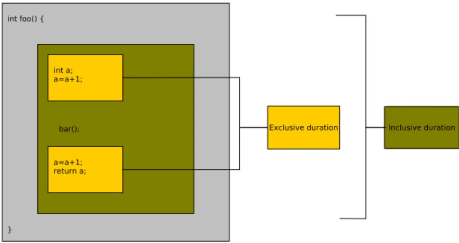
The most common way to analyze the performance of an application is the proőling of routine execution. Basically, proőling produce statistics for each routine call by the application indicating the number of times this routine is called and the time spent executing its code, including (or not) the time spent in calls to other routines. Figure 2.2 shows the exclusive and inclusive duration of a routine. The exclusive duration is the amount of time spent while within the foo function excluding the time spent in function bar which is called by foo. The inclusive

(17)

duration is the amount of execution time spent in foo, including the spent in all the busbroutines called by foo.

Accesses to times (or to hardware performance counters) are trivially made by inserting instrumentation probes at the beginning and ending of each routine as it can be seen in Figure 2.3 where a routine named main, calls a function foo with diferent argument values.

Figure 2.3: Instrumentation during proőling.

The advantage of proőles is that they can be calculated at run-time, require only a small amount of storage, and they can provide a generic glimpse of the application’s performance. However, we do not know exactly where a performance issue occurs. In the case of an iterative method, if there is a performance issue with some speciőc iterations we can not observe them. Note that proőles can be extracted through tracing by post-processing the produced trace, but the opposite is not possible.

2.2.4 Statistical Profiling

Statistical proőling or sampling probes the target program’s counter at regular intervals using operating system interrupts as we can see in Figure 2.4 where again a routine named main calls a routine foo with diferent arguments. Sampling proőles are less accurate and speciőc than full proőling, but allow the target program to run without inducing an instrumentation overhead. Usually this method is used for applications with long execution time where there is no need for detailed performance analysis.

(18)

2.3 Assessing the Performance of Applications on Resources

A user can not be aware of the performance of an application on speciőc resources if there is no interaction between them. This interaction can be done either by executing the application on the real platform, executing the application on a virtual environment that corresponds to the resources through emulation or simulating the application to predict its performance. These three approaches constitute the main ways to assess the performance of the applications on the resources and are detailed hereafter.

2.3.1 Experiments

Large-scale computer experiments are becoming increasingly important in science. An ex-periment can be executed on the available resources. Thus this is the most accurate approach for observing the performance of an application on the speciőc resources. Moreover it is possible through the experiment to observe some unexpected phenomena that a user was not aware of. Experiments also are important for validating theories. Experimentation in a real environment is expensive, because it requires a signiőcant number of resources available for a large amount of time. It also costs time, as it depends on the application to be actually deployed and exe-cuted under diferent loads, and for heavy loads long delays in execution time can be expected. Moreover the experiments are not repeatable, because a number of variables that are not under control of the tester may afect experimental results, and elimination of these inŕuences requires more experiments, making it even more time and resource expensive.

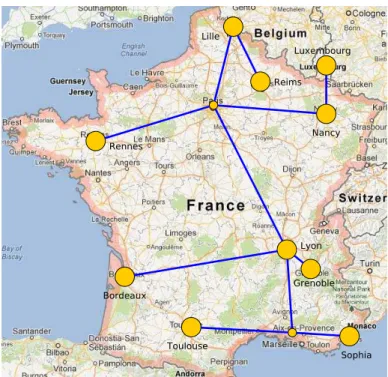
For all our direct experiments we used the Grid’5000 [39, 40] testbed. In 2003, several teams working around parallel and distributed systems designed a platform to support experiment-driven research in parallel and distributed systems. This platform, called Grid’5000 and opened to users since 2005, was solid enough to attract a large number of users. According to [41], this platform has led to a large number of research results: 575 users per year, more than 700 research papers, 600 diferent experiments, 24 ANR projects and 10 European projects and 50 PhD. Grid’5000 is located mainly in France (see Figure 2.5), with one operational site in Luxembourg and a second site, not ready yet, in Porto Alegre, Brazil. Grid’5000 provides a testbed supporting experiments on various types of distributed systems (high-performance computing, grids, peer-to-peer systems, cloud computing, and others), on all layers of the software stack. The core testbed currently comprises 10 sites. Grid’5000 is composed of 24 clusters, 1,169 nodes, and 8,080 CPU cores, with various generations of technology (Intel (56.2%), AMD (43.8%), CPUs from one to 12 cores, Myrinet, Inőniband and 2 GPU clusters). A dedicated 10 Gbps backbone network is provided by RENATER (the French National Research and Education Network).

From the user point of view, Grid’5000 is a set of sites with the same software environment. It provides to the users heterogeneity which can be controlled during the experiments. The main steps identiőed to run an experiment are (1) reserving suitable resources for the experiment and (2) deploying the experiment on the resources. The resource scheduler on each site is fed with the resource properties so that a user can ask for resources describing the required properties (e.g., 16 nodes connected to the same switch with at least 8 cores and 16 GB of memory). Once enough resources are found, they can be reserved either for exclusive access at a given time or for exclusive access when they become available. In the latter case, a script is given at reservation time, as in classical batch scheduling systems.

Several tools are provided to facilitate experiments. Most of them were originally developed speciőcally for Grid’5000. Grid’5000 users select and reserve resources with the OAR batch scheduler [42, 43]. Users can install their own system image on the nodes (without any

(19)

virtual-Figure 2.5: Presentation of the sites and the network of the Grid’5000 testbed.

ization layer) using Kadeploy [44]. Moreover the users can deploy a preconőgured environment on a node, called production environment.

2.3.2 Emulation

Emulation [45, 46] is an experimental approach allowing to execute real applications in a vir-tual environment. This allows us to reach the experimental settings wanted for an experiment. Most of the emulation solutions rely on a heavy infrastructure and mandate the use of a cluster and an emulation layer to reproduce the wanted environment. Emulators let unmodiőed appli-cations run in a speciőc environment where relevant system calls are intercepted and mediated. So basically an emulator is used to replace a system and execute an application on the virtual system.

There are many frameworks which propose their own emulator. The Emulab-Planetlab por-tal [47] allows to use the interface of the Emulab [48] emulator to access the Planetlab [49] experimental platform, to emulate applications based on this platform. This helps the scientists to emulate applications considering an existing platform. EMUSIM [50] integrates emulation and simulation environments in the domain of cloud computing applications and provides a framework for increased understanding of this type of systems. Furthermore, Netbed [48] is a platform based on Emulab that combines emulation with simulation to build homogeneous net-works using heterogeneous resources. Another emulator is Distem [51] which builds distributed virtual experimental environments. This tool is easily deployed on Grid’5000 platform and it can emulate a platform composed of heterogeneous nodes, connected to a virtual network described using a realistic topology model. An open problem is still the mapping of a virtual platform on a set of physical nodes. In the case that many virtual machines are on the same physical node there are limitations on the inter-node bandwidth and communication time that should be taken into account during the designing of the experiment.

(20)

2.3.3 Simulation

Simulation is a popular approach to obtain objective performance indicators on platforms that are not at one’s disposal. Simulation has been used extensively in several areas of computer science for decades, e.g., for microprocessor design and network protocol design. Moreover simulation can be used to evaluate a concept in early development stage. Simulations can also be used to study the performance behavior of an application by varying the hardware characteristics of a hypothetical platform. However, an application should be properly modeled, otherwise the simulation will not be accurate. A simulation is reproducible in comparison to real experiments or emulation. Furthermore, access to large-scale platforms is typically costly (possible access charges to the user, electrical power consumption). The use of simulation can not only save time but also money and resources.

The Message Passing Interface (MPI) is the dominant programming model for parallel sci-entiőc applications. Given the role of the MPI library as the communication substrate for application communication, the library must ensure to provide scalability both in performance and in resource usage. MPI development is active with an important role in the community and the new version MPI-3.0 [52] was released on September 2012 with intention to improve the scalability, performance and some other issues. Many frameworks for simulating the execution of MPI applications on parallel platforms have been proposed over the last decade. They fall into two categories: on-line simulation or łsimulation via direct executionž [53, 54, 55, 56, 57, 58, 59], and off-line simulation or łpost-mortem simulationž [60, 61, 62, 63, 64]. In on-line simulation the actual code, with no or only marginal modiőcation, is executed on a host platform that attempts to mimic the behavior of a target platform, i.e., a platform with diferent hardware characteristics. Although it is powerful, the main drawback of on-line simulation is that the amount of hardware resources required to simulate application execution at a given scale is com-mensurate to that needed to run the application on a real-world platform at that scale. Even though a few solutions have been proposed to mitigate this drawback and allow execution on a single computer [65, 66], the simulation time can be prohibitively high when applications are not regular or have data-dependent behavior. Part of the instruction stream is then intercepted and passed to a simulator. LAPSE is a well-known on-line simulator developed in the early 90’s [53] (see therein for references to precursor projects). In LAPSE, the parallel application executes normally but when a communication operation is performed a corresponding communication delay is simulated for the target platform using a simple network model (aine point-to-point communication delay based on link latency and bandwidth). MPI-SIM [54] builds on the same general principles, with the addition of I/O subsystem simulation. A diference with LAPSE is that MPI processes run as threads, a feature which is enabled by a source code preprocessor. Another project similar in intent and approach is the simulator described in [57]. The BigSim project [56], unlike MPI-SIM, allows the simulation of computational delays on the target plat-form. This makes it possible to simulate łwhat if?ž scenarios not only for the network but also for the compute nodes of the target platform. These computational delays are based either on user-supplied projections for the execution time of each block of code, on scaling measured exe-cution times by a factor that accounts for the performance diferential between the host and the target platforms, or based on sophisticated execution time prediction techniques such as those developed in [55]. The weakness of this approach is that since the computational application code is not executed, the computed application data is erroneous. Data-dependent behavior is then lost. This is acceptable for many regular parallel applications, but is more questionable for irregular applications (e.g., branch-and-bound or sparse matrices computations). Going further, the work in [58] uses a cycle-accurate hardware simulator of the target platform to simulate computation delays, which leads to a high ratio of simulation time to simulated time.

(21)

be-cause done through a direct execution of the MPI application, is inherently distributed. Parallel discrete event simulation raises diicult correctness issues pertaining to process synchronization. For the simulation of parallel applications, techniques have been developed to speed up the sim-ulation while preserving correctness (e.g., the asynchronous conservative simsim-ulation algorithms in [67], the optimistic simulation protocol in [56]). A solution could be to run the simulation on a single node but it requires large amounts of CPU and RAM resources. For most aforemen-tioned on-line approaches, the resources required to run a simulation of an MPI application are commensurate to those needed to run the application on a real-world platform. In some cases, those needs can even be higher [58, 59]. One way to reduce the CPU needs of the simulation is to avoid executing computational portions of the application and simulate only expected delays on the target platform [56]. Reducing the need for RAM resources is more diicult and if the target platform is a large cluster, then the host platform must then be a large cluster. SMPI [66], which builds on the same simulation kernel as this work, implements all the above techniques to allow for eicient single-node simulation of MPI applications.

An alternate approach is off-line simulation in which a log, or trace, of MPI communication events (time-stamp, source, destination, data size) is őrst obtained by running the application on a real-world platform. A simulator then replays the execution of the application as if it were running on a target platform. This approach has been used extensively, as shown by the number of trace-based simulators described in the literature since 2009 [60, 61, 62, 63, 64]. The typical approach is to decompose the trace in time intervals delimited by the MPI communication operations. The application is thus seen as a succession of computation bursts and communication operations. An of-line simulator then simply computes simulated delays in a way that accounts for the performance diferential between the platform used to obtain the trace and the platform to be simulated. Computation delays are typically computed by scaling the durations of the CPU bursts in the trace [61, 62, 64]. Network delays are computed based on a simulation model of the network. The main advantage when compared to on-line simulation is that replaying the execution can be performed on a single computer. This is because the replay does not entail executing any application code, but merely simulating computation and communication delays.

One limitation of these of-line simulators is that trace acquisition is not scalable. To simu-late the execution of an application on a platform of a given scale, the trace must be acquired on a homogeneous platform of that same scale, so that time-stamps are meaningful. In some cases, extrapolating a smaller trace to larger numbers of compute nodes is feasible [60], but not gen-erally applicable. Furthermore, the use of time-stamps requires that each trace be accompanied with a description of the platform on which it was obtained, so as to allow meaningful scaling of computation delays. In this work we address the trace acquisition scalability limitation by using time-independent traces.

Another limitation is that these simulators typically use simplistic network models, because they are straightforward to implement and scalable. Possible simpliőcations include: not using a network model but simply replay original communication delays [64]; ignoring network con-tention because it is known to be diicult and costly to simulate [60, 63, 68]; using monolithic performance models of collective communications rather than simulating them as sets of point-to-point communications [61, 64, 69]. Other simulators opt for accurate packet-level simulation, which is not scalable and leads to high simulation times [62].

One well-known challenge for of-line simulation is the large size of the traces, which limits the scalability of trace acquisition and can prevent running the simulation on a single node. Mech-anisms have been proposed to improve scalability, including compact trace representations [61] and replay of a judiciously selected subset of the traces [63].

(22)

application is łreplayedž on a simulated platform. SimG_rid

SimG_{rid [70] is a scientiőc instrument to study the behavior of large-scale distributed systems} such as Grids, Clouds, HPC or P2P systems. It can be used to evaluate heuristics, prototype applications or even assess legacy MPI applications. SimGrid was conceived as a scientiőc instrument, thus the validity of its analytical models was thoughtfully studied [71], ensuring their realism.

Some of the key features of SimGrid are:

ś A scalable and extensible simulation engine that implements several validated simulation models, and that makes it possible to simulate arbitrary network topologies, dynamic compute and network resource availabilities, as well as resource failures;

ś High-level user interfaces for distributed computing researchers to quickly prototype sim-ulations either in C or in Java;

ś APIs for distributed computing developers to develop distributed applications that can seamlessly run in łsimulation modež or in łreal-world modež.

SimGrid ofers four user interfaces as it can be seen in Figure 2.6.

Figure 2.6: SimGrid components.

MSG module provides an API for the easy prototyping of distributed applications by letting users focus solely on algorithmic issues. Simulations are constructed in terms of concurrent processes, which can be created, suspended, resumed and terminated dynamically, and can synchronize by exchanging data. Moreover it proved perfectly usable in other contexts, such as desktop grids [72]. An important diference between MSG and SMPI, is that all simulated processes are in the same address space. This simpliőes development of the simulation by allowing convenient communications via global data structures. In other words, while MSG can accurately simulate the interactions taking place in a distributed application, including communication and synchronization delays, the simulated application can be implemented with the convenience of a single address space.

SMPI [66] is a simulator for MPI applications. Its őrst version provided only on-line simu-lation, i.e., the application is executed but part of the execution takes place within a simulation component. In Chapter 4 we present our of-line simulator based on SMPI backend. SMPI

(23)

sim-ulations account for network contention in a fast and scalable manner. SMPI also implements an original and validated piece-wise linear model for data transfer times between cluster nodes. Finally SMPI simulations of large-scale applications on large-scale platforms can be executed on a single node thanks to techniques to reduce the simulation’s compute time and memory footprint.

SimDag is designed for the investigation of scheduling heuristics for applications as task graphs. SimDag allows to prototype and simulate scheduling heuristics for applications struc-tured as task graphs of (possibly parallel) tasks. With this API one can create tasks, add dependencies between tasks, retrieve information about the platform, schedule tasks for execu-tion on particular resources, and compute the DAG execuexecu-tion time.

SURF considers the platform as a set of resources, with each of the simulated concurrent tasks utilizes some subset of these resources. SURF computes the fraction of power that each resource delivers to each task that uses it by solving a constrained maximization problem: allocate as much power as possible to all tasks in a way that maximizes the minimum power allocation over all tasks, also called Max-Min fairness. SURF provides a fast implementation of Max-Min fairness. Via Max-Min fairness, SURF enables fast and realistic simulation of resource sharing (e.g., TCP ŕows over multi-link LAN and WAN paths, processes on a CPU). Furthermore, it enables trace-based simulation of dynamic resource availability. Finally, simulated platform conőgurations are described in XML using a syntax that provides an uniőed abstract basis for all other components of the SIMGRID project (MSG and SMPI).

XBT is a łtoolboxž module used throughout the software, which is written in ANSI C for performance. It implements classical data containers, logging and exception mechanisms, and support for conőguration and portability.

Now that the basic concepts of our work are analyzed, we can continue in the next chapter with the presentation of the time-independent trace acquisition framework.

(24)

Chapter 3

Time-Independent Trace Acquisition

Framework

All the of-line MPI simulators that were reviewed in 2.3.3, rely on timed traces, i.e., each occuring event is associated to a time-stamp. The duration of each computation or communi-cation operation is then deőned by the interval between two time-stamps. When it simulates an execution on a target platform that is diferent of the one used to get the trace, a simulator then has to apply a correction factor to these intervals. This implies to know precisely what are the respective characteristics of the host and target platforms. In other words, each execution trace must come with an accurate description of how it has been acquired. Finally, determining the right scaling factor can be tedious depending on the degree of similarity of both platforms. In this chapter we introduce a new of-line simulation framework, that free ourselves of time-stamps by relying on time-independent traces. For each event occurring during the execution of the traced application, e.g., a CPU burst or a communication operation, we log the volume of the operation (in number of instructions or bytes) instead of the time when it begins and ends. Indeed this type of information does not vary with the characteristics of the host platform. For instance, the size of the messages sent by an application is not likely to change according to the speciőcs of the network interconnect, while the computation amount performed within a for loop does not increase with the processing speed of a CPU. This claim is not valid for adaptive MPI applications that modify their execution path according to the execution platform. This type of applications, that represents only a small fraction of all MPI applications, is not covered by our work.

Another advantage of this approach is the lack of clock synchronization across all the par-ticipating nodes. This can be done because we do not need to extract the durations of the communications that occur during the execution of the parallel application. This is important as there can be many issues about clock synchronization [73] that are sometimes very diicult to identify.

A time-independent trace can been seen as a list of actions, e.g., computations and commu-nications, performed by each process of an MPI application. An action is described by the id of the process that does this action, a type, e.g., a computation or a communication operation, a volume, of instructions or bytes, and some action speciőc parameters such as the id of the receiving process for a one-way communication.

(25)

pos-sible to create the list of the actions which constitutes the time-independent traces. The only instrumented mode that provides analytic measurement data, is the tracing one. Thus we need a proőling tool that provides tracing functionalities.

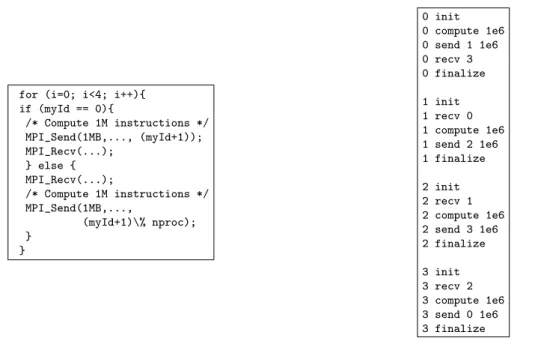
The left hand side of Figure 3.1 shows a simple computation executed on a ring of four processes. Each process computes one million instructions and sends one million bytes to its neighbor. The right hand side of this őgure displays the corresponding time-independent trace.

for (i=0; i<4; i++){ if (myId == 0){ /* Compute 1M instructions */ MPI_Send(1MB,..., (myId+1)); MPI_Recv(...); } else { MPI_Recv(...); /* Compute 1M instructions */ MPI_Send(1MB,..., (myId+1)\% nproc); } } 0 init 0 compute 1e6 0 send 1 1e6 0 recv 3 0 finalize 1 init 1 recv 0 1 compute 1e6 1 send 2 1e6 1 finalize 2 init 2 recv 1 2 compute 1e6 2 send 3 1e6 2 finalize 3 init 3 recv 2 3 compute 1e6 3 send 0 1e6 3 finalize

Figure 3.1: MPI code sample of some computation on a ring of processes (left) and its equivalent time-independent trace (right).

Note that, depending on the number of processes and the number of actions, it may be preferable to split the time-independent trace to obtain one őle per process. Indeed Figure 3.1 shows a simple example where all the actions can be included in the same őle. However, typical MPI applications are likely to be executed by dozen of processes that perform millions of actions each. Then it is often easier to split (or actually not merge as it will be explained later) the trace to have one őle per process, like in the Figure 3.2.

0 init 0 compute 1e6 0 send 1 1e6 0 recv 3 ... 0 finalize 1 init 1 recv 0 1 compute 1e6 1 send 2 1e6 ... 1 finalize ... 127 init 127 recv 2 127 compute 1e6 127 send 0 1e6 ... 127 finalize

Figure 3.2: Example of a split time-independent trace corresponding to a larger application execution with 128 processes.

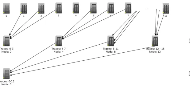
In this section we mention the main steps of the acquisition process. As it is shown in the Figure 3.3, in the beginning it is mandatory to instrument an application in order to record all the events that will occur during its execution. Afterwards, we execute the instrumented application on a parallel platform. Then from the acquired traces, we extract the time-independent traces, which are gathered into a single node.

(26)

Figure 3.3: Overview of the Time Independent Trace Replay Framework.

In order to replay the time-independent traces, the following requirements should apply. For the computation actions, we know the amount of instructions, and the processing speed of the CPU, so we can determine the time to complete the computation. However, some al-gorithms should be implemented for the communication actions in order to calculate the time needed to transfer the message from the sender to the receiver in the case of a point-to-point communication and similar for other type of communications. As there are no time-stamps in the execution traces, we should take under consideration the latency and the bandwidth of the network. Furthermore it is really important to simulate also the contention that may occur during the exchange of the data between the nodes. Thus, if a simulation model can handle all the mentioned factors, then it can use the time-independent traces in order to predict the performance of the corresponding application.

The remaining of this Chapter is organized as follows. Section 3.1 describes the instru-mentation of an application and evaluates some tracing tools. instruinstru-mentation methods. In Section 3.2, we evaluate the quality of diferent instrumentation methods in terms of overhead and skew. Section 3.3 details and evaluates the subsequent parts of the proposed trace acqui-sition framework. This presentation is illustrated by the deployment of our framework on the Grid’5000 platform. Finally, Section 3.4 concludes this chapter. Note that the replay of the time-independent traces will be covered in the next chapter.

3.1 Instrumenting an Application

Instrumenting an application to obtain an execution trace consists in adding probes to its code. For instance, such probes can be accesses to hardware counters or logs of the beginning and end of a function. Thanks to them, all the actions, i.e., computations or communications, can be traced in a chronological order. For every function enter/exit events are saved. The information which is logged for each event are the time-stamp, event type and event-related information such as the sender of a message, the receiver, etc. A crucial diference with other instrumentation modes such as proőling and statistical proőling, is that we know the chronologically ordered sequence of the events that occur during the execution.

The left-hand side of Figure 3.4 shows an example of what occurs during tracing. We have two processes, called A and B. The őrst one calls the function foo, sends a message to process B, and then exits. Similarly process B calls the function bar, receives a message from process A and exits. However, it is mandatory to monitor the time through a synchronization mechanism as we need to know when a communication starts and ends.

On the right-hand side of Figure 3.4, we can observe the sequence of events per process where the name of the functions and information on events are locally encoded. In the case of merged traces, we can observe the global sequence of events for both processes thanks to the recorded time-stamps and the synchronization. The uniőcation takes place to globally declare functions and other important information.

(27)

Figure 3.4: Example of tracing for two processes A and B that both call a function and exchange a message.

Our of-line simulation framework expresses the following requirements for time-independent traces:

ś For compute parts, the trace should contain the id of the process that executes the in-structions and the corresponding amount;

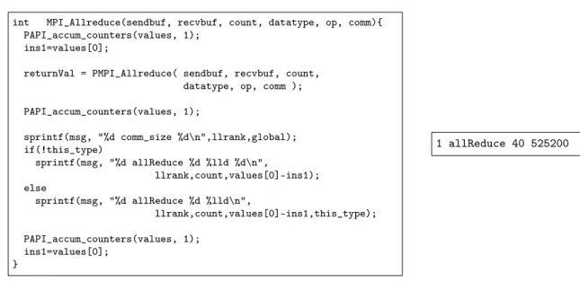
ś For point-to-point communications, it is mandatory to know both the sender and the receiver of the message, the type (MPI_Send, MPI_Recv, etc.) and the message size in bytes;

ś For collective communications, it is important to know at least the size of the message and the type of the MPI communication (MPI_Broadcast, etc.). However, there are some MPI calls such as MPI_Allreduce, where the participating processes execute also some computation, summing values or determining a maximum for example. In this case, it is mandatory to log the number of executed instructions in order to simulate the compute part;

ś For synchronization calls such as MPI_Barrier, it is mandatory to know the MPI Com-municator.

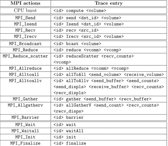
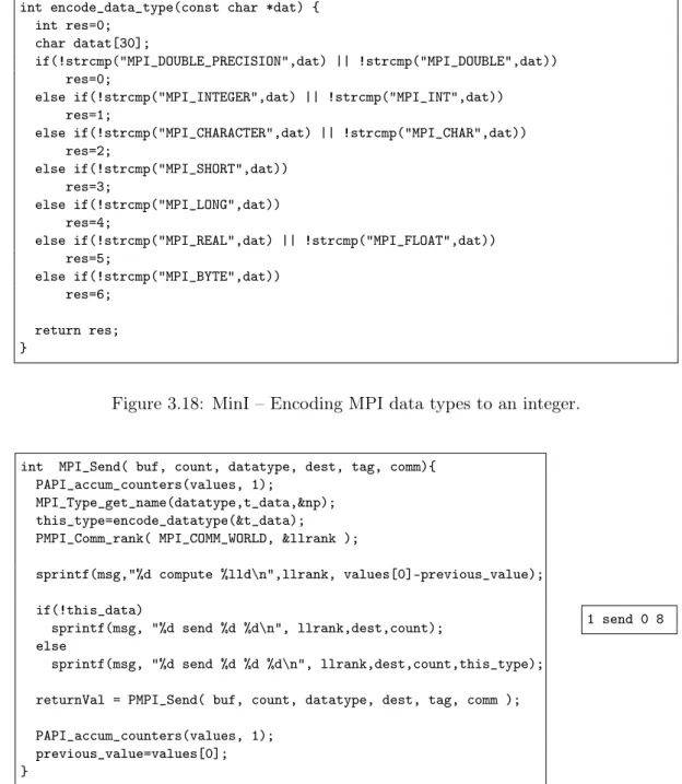
Currently our framework does not support all the MPI calls but the most common ones. Table 3.1 lists all the MPI functions for which there is a corresponding action implemented in our framework. For the collective operations, we consider that all the processes are involved as the MPI_Comm_split function is not implemented. When it is not possible to extract from the instrumented execution the information about the root process that initiates a collective operation, we assume that this process is the one of rank 0. Finally the init and finalize actions have to appear in the trace őle associated to each process to respectively create and destroy some internal data structures that will be needed during the replay of the traces.

3.1.1 Evaluation Criteria and Scoring Method

Many proőling tools can provide useful information about the behavior of parallel applica-tions and record the events that occur during their execution. PAPI[32] provides access to the

(28)

Table 3.1: Time-independent counterparts of the actions performed by each process involved in an MPI application.

MPI actions Trace entry

CPU burst <id> compute <volume> MPI_Send <id> send <dst_id> <volume> MPI_Isend <id> Isend <dst_id> <volume>

MPI_Recv <id> recv <src_id>

MPI_Irecv <id> Irecv <src_id> <volume> MPI_Broadcast <id> bcast <volume>

MPI_Reduce <id> reduce <vcomm> <vcomp> MPI_Reduce_scatter <id> reduceScatter <recv_counts>

<vcomp>

MPI_Allreduce <id> allReduce <vcomm> <vcomp>

MPI_Alltoall <id> allToAll <send_volume> <receive_volume> MPI_Alltoallv <id> allToAllv <send_buffer> <send_counts>

<send_displs> <receive_buffer> <recv_counts> <recv_displs>

MPI_Gather <id> gather <send_buffer> <recv_buffer> MPI_Allgatherv <id> allGatherV <send_count> <recv_counts>

<recv_disps> MPI_Barrier <id> barrier

MPI_Wait <id> wait MPI_Waitall <id> waitAll

MPI_Init <id> init MPI_Finalize <id> finalize

hardware counters of a processor. In our prototype framework we measured the compute parts of an application in numbers of ŕoating point operations (or ŕops). However, using another counter, such as the number of instructions, has no impact on the instrumentation overhead as long as the chosen measure does not combine the values of several counters. To select the tool that corresponds the most to the requirements expressed by our time-independent traces replay framework, we conducted an evaluation based on the following criteria and scoring method: Profiling Features

Many tools exist to proőle parallel applications, i.e., get an idea of the behavior of the application over its execution time. A classiőcation of these tools can be made following two axes. The őrst distinction depends on the type of output produced by the considered tool. It can be either a profile or a trace. A proőle gives a higher view of the behavior of an application as information is grouped according to a type of operation or to the call tree. A trace gives lower level information as every event is logged without any aggregation. The second way to classify tools depends on the kind of events they can be proőled or traced. Such events are mainly related to communication or computation. A third important parameter for this evaluation is the type of value associated to each logged event, e.g., volumes or timings. Finally, the instrumentation of an application is mandatory to obtain a proőle or a trace. Such a instrumentation can be applied to the entire application or to a speciőc block of code, e.g., , a particular function or a MPI call. In this evaluation we give a higher score to tools ofering an automatic instrumentation

(29)

feature. Such a feature lighten the burden of getting a proőle from a user point of view. With regard to the speciőc requirements of our time-independent trace replay framework, we adopt the following scoring scheme for the Profiling feature criterion:

ś Tracing → 2 points

ś Information on communication →1 point

ś Information on computation →1 point

ś Information on communication volumes (in bytes) →1 point

ś Information on computation volumes (in ŕops) →1 point

ś Automatic instrumentation of the complete application →1 point

ś Automatic instrumentation of a block of code →1 point

Each tool can then obtain a score ranging from 0 to 8, the higher being the better. Quality of Output

Proőling tools usually output the results in őles. These őles could be of various formats such as plain text, XML, or binary formats. As mentioned earlier our objective is to convert such output őles into set of actions to be replayed by SimGrid. The readability of the output őles is then a very important requirement. However, tools that produce binary őles often come with an application or an API to extract the required information. Finally we aim at replaying executions that involve large numbers of processes. To ensure a good scalability, it is important that the trace of each process is stored in a separate őle. Indeed a tool enforcing a unique trace őle for the complete execution will have a poor scalability due to merging overhead. Moreover as we intend to read these traces and extract the time-independent ones, if there is at least one trace őle per node, then we can use the same number of nodes with a parallel application to achieve our purpose. This means that even for large trace sizes we would be able to use many processors and hard disks. So the conversion will be much faster than using just one node. Then we propose the following scoring scheme (ranging from 0 to 3) for the Output quality criterion:

ś Capacity to extract the required information →1 point

ś Direct extraction →1 point

ś One pass conversion →1 point

Space and Time Overheads

As already mentioned, őles that contain all the relevant information are created during the tracing or proőling of an application. Proőling provides aggregated data about an application. This means for example that it records the number of times a function is called and its average duration. Conversely tracing records each call independently with the timestamp and some other information which depend on what the user wants to measure. The source of the time overhead for an instrumented application are the measurement of a PAPI counter on the processor, the instrumentation of the MPI communications, and writing traces on disks. In terms of space overhead, proőling obviously leads to smaller traces, as logged events are aggregated.

Then, for Space and Time overhead, we adopt the following scoring scheme:

ś Overhead < 50% of the initial execution time → 2 points

ś 50% < Overhead < 100% of the initial execution time →1 point The executed time of the instrumented application includes the time needed to write the produced traces on disk.

ś Linear increase of the overhead →1 point

ś Constant overhead → 2 points

ś Linear decrease of the overhead → 3 points