A Geometric Approach to the Landauer-Büttiker Formula

(1)

HAL Id: hal-00943060

https://hal.archives-ouvertes.fr/hal-00943060

Submitted on 6 Feb 2014

HAL is a multi-disciplinary open access

archive for the deposit and dissemination of sci-entific research documents, whether they are pub-lished or not. The documents may come from teaching and research institutions in France or

L’archive ouverte pluridisciplinaire HAL, est destinée au dépôt et à la diffusion de documents scientifiques de niveau recherche, publiés ou non, émanant des établissements d’enseignement et de recherche français ou étrangers, des laboratoires

Formula

Rym Ben Sâad, Claude-Alain Pillet

To cite this version:

Rym Ben Sâad, Claude-Alain Pillet. A Geometric Approach to the Landauer-Büttiker For-mula. Journal of Mathematical Physics, American Institute of Physics (AIP), 2014, 55, pp.075202. �10.1063/1.4879238�. �hal-00943060�

(2)

Landauer-Büttiker Formula

R. B

EN

S

ÂADa

, C.-A. P

ILLETb

a_{Laboratoire Mathématiques et Applications, INSAT Centre Urbain Nord BP 676, 1080 Tunis Cedex}

b_{Aix-Marseille Université, CNRS, CPT, UMR 7332, Case 907, 13288 Marseille, France}

Université de Toulon, CNRS, CPT, UMR 7332, 83957 La Garde, France FRUMAM

con-sisting of a central region – the sample – connected to several infinitely extended ends – the reservoirs. Under physically reasonable assumptions on the propaga-tion properties of the one-particle dynamics within these reservoirs, we show that the state of the Fermi gas relaxes to a steady state. We compute the expected value of various current observables in this steady state and express the result in terms of scattering data, thus obtaining a geometric version of the celebrated Landauer-Büttiker formula.

1 Introduction

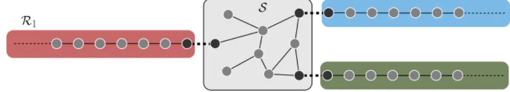
The study of transport phenomena in the quantum regime has attracted a lot of interest over the last decades, especially within the realm of condensed matter physics. The main efforts have been devoted to the development of computational tools for the calculation of steady state properties of a confined quantum system (the sample) driven out of thermal equilibrium by mechanical or thermodynamical forces. This physical setup is conveniently described by an open-system model where the sample S is coupled to large (eventually infinitely ex-tended) heat and particle reservoirs R1,R2,... (see Figure 1). Thermodynamical forces are

implemented by the initial state of the joint system S + R1+ R2+ ···. More precisely, each

reservoir Rkis prepared in a thermal equilibrium state with its own intensive thermodynamic

parameters: inverse temperature βk, chemical potential µk,. . . In the physics literature, this is

sometimes called “the partitioned scenario”, reflecting the fact that each reservoir has to be prepared individually before being connected to the sample. Mechanical forcing is obtained by imposing (possibly time dependent) potential bias in the reservoirs, the initial state of the system being a joint thermal equilibrium state of the coupled system S + R1+ R2+ ···. This

is the so called “partition free scenario”, see [CCNS,C].

Whether such an open system, prepared in a given initial state, actually relaxes to a steady state is a more delicate question which can not be treated by formal arguments and requires a precise control of quantum dynamics. To the best of our knowledge, the first rigorous re-sults on this fundamental problem of nonequilibrium quantum statistical mechanics were obtained by Lebowitz and Spohn [Sp1, Sp2, Sp3, LS] in the case of thermodynamical forc-ing. Besides providing simple and efficient criteria ensuring relaxation to a steady state in the van Hove scaling limit (weak coupling), they have also studied the basic thermodynamic properties of these steady states: strict positivity of entropy production and linear response

(6)

S

RM

R₁

R₂

Rk

Figure 1: A sample S coupled to M reservoirs R1,...,RM.

theory. In the same limit, Davies and Spohn have studied the linear response of confined quantum systems to mechanical drives [DSp]. These works rely on Davies’ results on the weak coupling limit [D1,D2] (see also the recent extension of Davies’ theory by Derezi´nski and de Roeck [DdR1,DdR2]) and therefore only provide a coarse time resolution of transport phenomena.

In these notes we shall consider the simplest case, beyond the weak coupling limit, amenable to rigorous analysis: the transport properties of an ideal Fermi gas (e.g., of an electronic gas in the approximation of independent electrons commonly used in solid state physics). Due to the absence of interactions, the nonequilibrium properties of such a gas can be derived from the quantum dynamics of a one-particle system. We shall concentrate more specifically on the Landauer-Büttiker formalism which relates the steady currents through a sample con-nected to several fermionic reservoirs at different chemical potentials to the scattering data associated with the coupling of the sample to the reservoirs (we shall provide a more detailed discussion of the Landauer-Büttiker formalism in Section3.4.7).

Relaxation to a nonequilibrium steady state (NESS) for an ideal Fermi gas in the partitioned scenario was first obtained by Araki and Ho [AH]. These Authors studied the large time asymp-totics of the isotropic XY spin chain prepared in a state with different temperatures on its left and and right ends (the XY chain can be mapped to an ideal Fermi gas on a 1D lattice by a Jordan-Wigner transformation). Their result has been extended to the anisotropic XY chain in [AP] using a different approach, advocated by Ruelle [R4], and based on scattering theory. In Ruelle’s approach, the NESS is expressed in terms of the initial state of the gas and the Møller operator describing the scattering of a particle from the reservoirs by the sample (see Section5.5). However, to derive the Landauer-Büttiker formula which expresses the steady state currents in terms of transmission probabilities (i.e., scattering matrix) requires further work. This was first achieved in [AJPP2,N] within the stationary formalism of scattering the-ory and for more general classes of ideal Fermi gases driven by thermodynamical forces (see also Section 7 in [AJPP1] and [CNWZ]).

In the case of mechanical forcing (in the partition-free scenario), a linearized Landauer-Büt-tiker formula (i.e., a formula for the conductivity of the sample) was obtained by Cornean et al. in [CJM,CDNP]. However, relaxation to a NESS did not follow from the linear response

(7)

approach used in these works and was first proved in [CDP]1. Finally, a complete (non-linear) Landauer-Büttiker formula for the steady currents was derived in [CGZ]. A unified treatment of the partitioned/partition-free NESS can be found in [CMP2].

In both scenarios a necessary condition for the coupled/biased system S + R1+ ··· to relax

to a NESS is that its final, fully coupled/biased, one-particle Hamiltonian has empty singular spectrum. In that case, the NESS only depends on the initial states of the reservoirs and on the final one-particle Hamiltonian. It is, in particular, independent of the initial state of the sample and of the (possibly time-dependent) switching of the coupling/bias [CNZ,CMP2]. In fact, the presence of eigenvalues in the one-particle Hamiltonian of the fully coupled/biased system produces oscillations which prevent relaxation to a steady state [Ste,KKSG]. These oscillations are carried by the eigenfunctions of the Hamiltonian and hence are typically lo-calized near the sample. Current measurements performed deep into the reservoirs are there-fore immune to this effect [CGZ]. If the singular continuous spectrum of the final Hamilto-nian is empty, then the oscillations induced by its eigenvalues can also be washed out by time-averaging the state of the system. The time-averaged state relax to a steady state which, however, depends on the initial state of the sample and on the history of the coupling/bias [AJPP2,CGZ,CJN].

Before turning to a detailed review of the content of these notes, let us mention some impor-tant results in the same line of research but which will not be covered here.

Ruelle’s scattering approach also works in the presence of weak local interactions (i.e., many body interactions that are sufficiently well localized in position and momentum). In this case, the Møller operator of Hilbert space scattering theory is replaced by a Møller morphism act-ing on the C∗_{-algebra O of observables of the coupled system (O is typically the gauge}

in-variant part of the C∗_{-algebra generated by fermionic creation/annihilation operators}

sat-isfying the canonical anti-commutation relations, see Section3.2). This morphism can be constructed by controlling the Dyson expansion of the interaction picture propagator act-ing on O, usact-ing the techniques of [BM1, BM2]. Relaxation to a NESS of a locally interact-ing Fermi gas in the partitioned scenario was first proved by Fröhlich et al. [DFG, FMU]. Linear response theory (including a central limit theorem) for such NESS was developed in [JOP1,JOP2,JPP]. Using similar techniques, a mathematical theory of basic thermodynamic processes in ideal and locally interacting Fermi gases has been developed in [FMSU]. A uni-fied approach to both partitioned/partition-free NESS of locally interacting Fermi gases was developed in [CMP1,CMP2] where basic properties of the NESS Green-Keldysh correlation functions were also derived.

The spectral analysis of Liouvilleans provides an alternative to Ruelle’s scattering approach to the construction of NESS. A Liouvillean for the coupled system S + R1+ ··· is an operator L

acting on a Hilbert space which carries a representation of the C∗_{-algebra O and such that the}

group t 7→ eitL implements the dynamics (see [P2,DJP,JOPP]). For systems with finitely ex-tended reservoirs the Liouvillean is essentially determined by the Hamiltonian. There is

how-1_{For identical intensive thermodynamic parameters, the partitioned/partition-free scenarios lead to distinct}

(8)

ever much more freedom in the choice of a Liouvillean if the reservoirs are infinitely extended. The Liouvillean approach has been successfully used to prove return to equilibrium of a con-fined system connected to a single heat bath [JP1,JP2,JP3,JP4,Me,BFS3,DJ1,DJ2,FM]. An extension of this technique to nonequilibrium situations was developed in [JP6] to prove re-laxation to a steady state of a N-level system coupled to several fermionic reservoirs. Merkli, Mück and Sigal have extended this result to the technically more involved case of bosonic reservoirs [MMS]. In these works, the steady state is characterized by a spectral resonance of a Liouvillean which is constructed with the help of operator algebraic techniques derived from the fundamental results of [HHW,To,Ta]. Due to the use of spectral deformation tech-niques in the resonance analysis, the method requires quite strong regularity assumptions on the coupling of the sample to the reservoir. It does however provide a very detailed infor-mation on the dependence of the NESS on this coupling (a convergent perturbative expan-sion). A similar approach was used by Fröhlich, Merkli and Sigal [FMS] to study the ionization process in a thermal field. We shall also mention a series of works by Abou Salem and Fröh-lich [AF1, AF2,AF3] who exploit the Liouvillean approach to derive some of the basic laws of thermodynamics from microscopic quantum dynamics. We refer the reader to the article of Schach Møller [SM] in this volume for a detailed exposition of the spectral theory of some important classes of Liouvilleans.

A third approach to the relaxation problem has been developed by de Roeck and Kupiainen in [dRK1,dRK2] (see also [dR1]). It uses Davies’ weak coupling approximation of the dynamics as a starting point for a systematic expansion of the true, fully coupled dynamics. The control of this expansion is technically more involved than the analysis required in the Liouvillean approach, but it is very robust and only requires minimal assumptions on the coupling to the reservoir (essentially the existence of the Davies approximation with a spectral gap). How-ever, the method does not provide much information on the dependence of the NESS on the coupling.

The material presented in these notes is partly based on the PhD thesis of the first Author [Sa]. It can be read as a pedagogical introduction to some contemporary aspects of the mathemat-ics of nonequilibrium quantum statistical mechanmathemat-ics. The main objectives are:

• To prove relaxation of an ideal Fermi gas under thermodynamical drive using Ruelle’s approach and geometric time-dependent scattering theory based on the Mourre esti-mate. This framework has many advantages over the stationary scattering theory used in the previous works on the subject. Our main assumptions, which ensure good prop-agation properties at large distance from the sample, concerns the reservoirs. They are easily checked for reservoirs with a simple geometry. Mourre theory gives us a simulta-neous control over the propagation properties and the singular spectrum of the coupled system. Finally, with the use of the two Hilbert space formalism, we avoid the decou-pling of the sample by artificial boundary conditions. The scattering matrix obtained in this way is explicitly independent of any decoupling scheme, which represents a serious conceptual advantage.

(9)

• To show that the properly defined NESS expectation of a current observable can be ex-pressed in terms of scattering data by a geometric version of the Landauer-Büttiker for-mula. Our approach has been deeply inspired by the works of Avron et al. [AEGS1, AEGS2,AEGS3] and more specifically [AEGSS] who treat the similar problem of charge transport in quantum pumps in the adiabatic regime (and prove the Büttiker-Prêtre-Thomas formula [BTP]).

Our main results are Proposition5.14and Theorem5.15, which guarantee the existence and uniqueness of the NESS under physically reasonable conditions. Under a few additional as-sumptions, we prove a geometric version of the Landauer-Büttiker formula in Theorem6.7.

The organization of these notes is as follows:

• In Section2we describe the necessary mathematical background for our work. The goal here is essentially to introduce the basic tools and the notation that will be used in the following sections.

• Section3is a brief introduction to nonequilibrium statistical mechanics of open quan-tum systems, and more specifically, -free fermionic systems. We introduce the concept of NESS and describe Ruelle’s scattering method for its construction.

• Section4is a thorough discussion of commutators of Hilbert space operators and their use in spectral analysis. It introduces the elements of Mourre theory which will be nec-essary for controlling the singular spectrum and the propagation properties of quasi-free fermionic systems.

• Section5is dedicated to the construction of NESS using the geometric theory of multi-channel scattering and propagation estimates.

• In Section6we discuss current observables and compute their expectation values in the NESS, deriving the geometric Landauer-Büttiker formula.

• The appendicesAandBcontain a few technical proofs that we deemed appropriate to be separated from the main part of these notes.

Acknowledgments. This work was partly supported by ANR (grant 09-BLAN-0098). We are

grateful to Y. Barsheshat for his help in translating parts of the PhD thesis of the first Author included in this notes. C.-A.P. is also grateful to V. Jakši´c, to the Department of Mathematics and Statistics at McGill University and to CRM (CNRS - UMI 3457) for hospitality and generous support during his stay in Montreal where parts of this work were done.

(10)

2 Mathematical background

In this section we briefly review the necessary mathematical background. The main purpose is to setup our notation. The covered material is very basic and the exposition is in telegraphic style, without formal proofs. The readers familiar with spectral analysis in Hilbert spaces and operator algebras can safely jump over to the next section.

In Subsection2.1we introduce the fundamentals of spectral analysis of operators on a Hilbert space, paying particular attention to self-adjoint operators and to the scattering theory of the associated unitary groups. These are the common tools used in the mathematical study of quantum dynamics, i.e., solutions to the Schrödinger equation, either time-dependent or time-independent. Among the numerous techniques developed to study the properties of the solutions to this equation, those based on the work of Mourre will play a central role in these notes. These techniques will be the object of a more detailed discussion in Section4.

Subsection2.2is a brief introduction to the theory of operator algebras and more particularly

C∗-algebras. From the perspective of the material covered in these notes, the relevance of this subject is marginal. It does however play an important role in the more general context of the mathematical theory of quantum statistical mechanics. As we have already noted in the gen-eral introduction, the development of this theory saw a revival in the last decade, essentially revolving around transport problems in nonequilibrium systems. These recent developments were built upon the foundations of the algebraic approach to equilibrium quantum statistical mechanics developed in the 1960s and 1970s.

2.1 Spectral analysis and scattering theory

In this section we recall some fundamental results of spectral analysis of self-adjoint operators on a Hilbert space, as well as the basics of scattering theory. The material covered in this section is treated in full detail in [RS1]–[RS4].

2.1.1 Closed operators and bounded operators

If A,B are non-empty sets we denote by 〈a,b〉 the elements of the Cartesian product A × B so as to not generate confusion with the following notation.

Let H be a Hilbert space. We denote by

H _{× H −→} C

〈u, v〉 7→ (u, v),

the inner product of H , which is anti-linear in its first argument and linear in its second one. Riesz’ representation theorem guarantees that any continuous linear functional ℓ : H → C can be written in the form ℓ(v) = (u,v) for some u ∈ H . The ortho-complement of a sub-set V ⊂ H is defined by V⊥_{= {u ∈ H |(v,u) = 0 for all v ∈ V }. It is a closed subspace of H}

(11)

linear and isometric bijection from H onto itself. H × H equipped with its natural vector space structure and the inner product (〈u,v〉,〈u′_{, v}′_{〉) = (u,u}′_{) + (v,v}′_{) is a Hilbert space and}

K: 〈x, y〉 7→ 〈y,x〉 and J : 〈x, y〉 7→ 〈−y,x〉 define automorphisms of H × H . A net u_α in H converges weakly to u ∈ H if the net (v,uα) converges to (v,u) for all v ∈ H . In this case we

write

w − lim_α uα= u.

An operator on H is a linear map A : D → H , where D is a subspace of H . We say that D is the domain of A which we denote by Dom(A). A is densely defined if its domain is dense in H. The range and the kernel of A are the subspaces Ran(A) ≡ {Au |u ∈ Dom(A)} and Ker(A) ≡ {u ∈ Dom(A)| Au = 0} respectively. A is surjective if Ran(A) = H and injective if Ker(A) = {0}. The graph of an operator A on H is the the subspace

Gr(A) ≡ {〈u, Au〉|u ∈ Dom(A)},

of H × H . The graph norm of A is the norm defined by kukA= kuk + kAuk on Dom(A). An

operator A is completely characterized by its graph. Moreover, a subspace G ⊂ H × H is the graph of an operator iff 〈0,v〉 ∈ G implies v = 0. If A and B are two operators such that Gr(A) ⊂ Gr(B) we say that B is an extension of A and we write A ⊂ B. An operator A is closed if its graph is closed in H ×H , and this is the case iff Dom(A), equipped with the graph norm of A, is a Banach space. If A is both closed and bijective, then Gr(A−1_{) = KGr(A) and thus A}−1

is also closed. If the closure Gr(A)cl of the graph of A in H × H is a graph we say that A is closable and we define its closure as the operator Acl_{such that Gr(A}cl_{) = Gr(A)}cl_{. It is clear}

that Aclis the smallest closed extension of A, that is to say that if B is closed and A ⊂ B, then

Acl_{⊂ B. An operator A is densely defined iff J(Gr(A)}⊥) is a graph. In this case, the adjoint of

A is the operator A∗defined by Gr(A∗) = J(Gr(A)⊥). A∗is closed and its domain is given by

Dom(A∗_{) = {u ∈ H |} _sup

v∈Dom(A),kvk=1|(u, Av)| < ∞}.

(A∗_{u, v) = (u, Av) holds for all 〈u, v〉 ∈ Dom(A}∗_{) × Dom(A), in particular Ker(A}∗_{) = Ran(A)}⊥_.

A is closable iff A∗is densely defined. In this case Acl= A∗∗and Acl∗= A∗.

An operator A is bounded if there exists a constant C such that Gr(A) ⊂ {〈u,v〉|kvk ≤ Ckuk}. One easily verifies that A is continuous as a map from Dom(A) to H iff it is bounded. A bounded operator is obviously closable and its closure coincide with its unique continuous extension to the closure of Dom(A). In particular a bounded densely defined operator A has a unique continuous extension Aclwith domain Dom(Acl) = H . Aclis closed and bounded. The collection of all bounded operators with domain H is denoted by B(H ). It is a Banach algebra (actually a C∗_{-algebra, see Section}_2.2_{) with norm}

kAk ≡ sup

u∈H ,kuk=1kAuk.

(1) By the closed graph theorem, an operator A with domain H is bounded iff it is closed. If A is bounded and densely defined, then Dom(A∗_{) = H and A}∗ _{is bounded. Furthermore,}

(12)

A bounded net Aα in B(H ) is strongly (resp. weakly) convergent if the net Aαu is

conver-gent (resp. weakly converconver-gent) for every u ∈ H . In this case, there exists A ∈ B(H ) such that limαAαu = Au for all u ∈ H (resp. limα(u, Aαv) = (u, Av) for all u, v ∈ H ), and we

write s − limαAα= A (resp. w − limαAα= A). If A(1)α ,..., A(n)α are bounded nets in B(H ) and

s − limαA(j )α = A(j )for all j then s − limαA(1)α ··· A(n)α = A(1)··· A(n).

The resolvent set of a closed operator A is defined by

Res(A) = {z ∈ C|Ker(A − z) = {0} and Ran(A − z) = H },

thus z ∈ Res(A) if and only if (A − z) : Dom(A) → H is a bijection. In this case, the operator

RA(z) ≡ (A − z)−1: H → Dom(A) is called the resolvent of A at z. It is a closed operator with

domain H , and is thus bounded. It satisfies the functional equation RA(z) − RA(z′) = (z −

z′)RA(z)RA(z′) (so called first resolvent equation) for all z, z′∈ Res(A). If follows that for z0∈

Res(A) RA(z) = ∞ X n=0 RA(z0)n+1(z − z0)n,

this Neumann series being norm convergent for |z − z0| < kRA(z0)k−1. Thus, the resolvent set

of A is open, and the mapping z 7→ RA(z) is an analytic function from Res(A) to B(H ). The

closed set Sp(A) ≡ C \ Res(A) is called the spectrum of A. A point a ∈ Sp(A) is an eigenvalue of A if there exists a non-zero vector u ∈ Dom(A) such that Au = au. We say that u is an eigenvector of A associated to the eigenvalue a.

If H and K are two Hilbert spaces, most of the preceding facts easily generalize to linear maps A from Dom(A) ⊂ H to K . We denote by B(H ,K ) the Banach space of continuous operators from H to K equipped with the norm (1).

2.1.2 Self-adjoint operators

An operator A is called symmetric if A ⊂ A∗_{, self-adjoint if A = A}∗_{, and essentially self-adjoint}

if A∗∗_{= A}∗_{. An essentially self-adjoint operator A is closable and its closure A}cl_{= A}∗∗_is

self-adjoint. In this case, we say that Dom(A) is a core of Acl.

An operator A is symmetric if and only if (u, Au) ∈ R for all u ∈ Dom(A). Such an operator is self-adjoint iff Ran(A ± i) = H and it is essentially self-adjoint iff Ran(A ± i) is dense in H . If K is a closed subspace of H then H = K ⊕ K⊥_{, i.e., any u ∈ H has a unique}

representa-tion u = x + y with x ∈ K and y ∈ K⊥_{. Moreover the Pythagoras theorem kuk}2_{= kxk}2_{+ kyk}2

holds. The decomposition u = x + y defines a bounded operator P : u 7→ x satisfying P =

P2_{= P}∗_{. We call P the orthogonal projection onto K . Note that Q = I − P is the orthogonal}

projection onto K⊥_{. Reciprocally, if P ∈ B(H ) satisfies P = P}2_{= P}∗_{then it is the orthogonal}

projection onto the closed subspace Ran(P) = Ker(I −P) and I −P is the orthogonal projection onto Ker(P) = Ran(I − P).

If K is a closed subspace of H and J is an operator with domain H such that kJuk = kuk for all u ∈ K and Ju = 0 for all u ∈ K⊥_{then Ker(J) = K}⊥_{and R ≡ Ran(J) is a closed subspace}

(13)

of H . J is thus a isometric bijection from K into R. We say that J is a partial isometry with initial space K and final space R. One verifies that J J∗ _{is the orthogonal projection onto}

R _{and J}∗_{J is the orthogonal projection onto K . If K = R = H then J J}∗_{= J}∗_{J = I and J is} unitary.

If A is self-adjoint, then Sp(A) ⊂ R. If we also have that Sp(A) ⊂ [0,∞[, then A is called positive and we write A ≥ 0. A self-adjoint operator is positive if and only if (u, Au) ≥ 0 for all u ∈ Dom(A). If C is a closed operator then C∗_{C with the domain Dom(C}∗_{C ) = {u ∈ Dom(C )|Cu ∈}

Dom(C∗_{)} is positive. Conversely, every positive operator is of this form.}

Every closed operator A has a unique polar decomposition A = J|A| where |A| ≥ 0 and J is a partial isometry with initial space Ran(A∗₎cl_{= Ker(A)}⊥_{and final space Ran(A)}cl

= Ker(A∗)⊥. Moreover, |A| is the square root of the positive operator A∗_{A constructed with the help of}

functional calculus which we shall now describe.

Spectral theorem 1. Let Bb(R) be the algebra of bounded Borel functions from R to C. If A is

self-adjoint, there exists a unique morphism φA: Bb(R) → B(H ) such that

(i) φA(f ) = φA(f )∗.

(ii) kφA(f )k ≤ sup_a∈Sp(A)|f (a)|.

(iii) If limnfn(a) = f (a) for all a ∈ Sp(A) and sup_n,a∈Sp(a)|fn(a)| < ∞ then

lim

n φA(fn)u = φA(f )u,

for all u ∈ H .

(iv) If f ≥ 0 then φA(f ) ≥ 0.

(v) If Au = au then φA(f )u = f (a)u.

(vi) If z ∈ Res(A) and f (a) = (a − z)−1_{then φ}

A(f ) = RA(z).

We call this morphism the functional calculus associated with A and we write f (A) = φA(f ).

We say that a bounded operator B commutes with A if B f (A) = f (A)B for all f ∈ Bb(R). A

subspace K ⊂ H is A-invariant if f (A)K ⊂ K for all f ∈ Bb(R). It reduces A if in addition

K⊥is also A-invariant. If K reduces A we define the part of A in K to be the self-adjoint operator on Dom(A) ∩ K obtained by restricting A to this subspace. We also define the part of the spectrum of A in K as Sp(A|K ) ≡ Sp(A|K_∩Dom(A)).

Spectral theorem 2. It follows from the functional calculus that for all u ∈ H the map f 7→

(u, f (A)u) is a continuous linear functional on C_∞(R), the Banach space of continuous func-tions from R to C which tend to 0 at infinity, equipped with the norm kf k∞≡ supx∈R|f (x)|.

The Riesz-Markov theorem implies that there exists a finite measure µu, with µu(R) = kuk2,

and such that

(u, f (A)u) = Z

(14)

µuis the spectral measure of A associated with u.

Let u ∈ H and Hu= {f (A)u | f ∈ C∞(R)}cl. The map f 7→ f (A)u from C∞(R) → Hu satisfies

kf (A)uk = kf kL2(R,dµu). It extends continuously to a unitary operator Uu : L

2_(R,dµ

u) → Hu

such that, if Mg denotes the multiplication operator f 7→ g f on L2(R,dµu), UuMg = g (A)Uu.

If H is separable, one can easily show that there exists a countable family (un)n∈N⊂ H such

that H = ⊕n∈NHun. In this way we obtain a unitary map U : ⊕n∈NL

2_(R,dµ

n) → H such that,

if g denotes the operator ⊕nun7→ ⊕ng un, then Ug = g(A)U. Alternatively stated, A is unitarily

equivalent to the operator of multiplication by the variable a in the space ⊕n∈NL2(R,dµn(a)).

One can show that H = Hpp(A) ⊕ Hac(A) ⊕ Hsc(A) where

H_pp(A) ≡ {u ∈ H |µ_uis purely atomic} ∪ {0},

H_ac(A) ≡ {u ∈ H |µ_uis Lebesgue-absolutely continuous} ∪ {0}, H_sc(A) ≡ {u ∈ H |µ_uis Lebesgue-singular without atoms} ∪ {0},

are mutually orthogonal subspaces reducing A. We denote by Ppp(A), Pac(A) and Psc(A) the

orthogonal projections onto these subspaces and we define App, Aac, and Ascto be the parts

of A in each of these subspaces. Hpp(A) is the subspace spanned by the eigenvectors of A.

The pure point, absolutely continuous, and singular spectra of A are defined by Sp_pp(A) ≡ {a ∈ R|a is an eigenvalue of A},

Sp_ac(A) ≡ Sp(Aac),

Sp_sc(A) ≡ Sp(Asc),

and we have that Sp(A) = Sppp(A)cl∪ Spac(A) ∪ Spsc(A).

The singular spectrum of A is Sp_sing(A) = Sppp(A)cl∪ Spsc(A). Its discrete spectrum is the

set Sp_disc(A) of all its isolated eigenvalues a having finite multiplicity, i.e., such that the corre-sponding eigenspace Ker(A−a) is finite dimensional. The essential spectrum of A is Spess(A) =

Sp(A) \ Sp_disc(A).

Spectral theorem 3. If 1∆is the indicator function of a Borel set ∆ ⊂ R, then EA(∆) ≡ 1∆(A) is an

orthogonal projection. It is the spectral projection of A associated with ∆. Its image reduces

A and we have that Sp(A|RanE∆(A)) = Sp(A) ∩ ∆ ⊂ ∆ and Sp(A|KerE∆(A)) ∩ ∆ is empty. The

family {E∆(A)|∆ ⊂ R measurable} is called the spectral family of A. Stone’s formula relates the

spectral family to the resolvent of A: for all u ∈ H one has 1

2(EA([a,b]) + EA(]a,b[))u = limε↓0

1 2πi

Zb a

(RA(a + iε)u − RA(a − iε)u) da, (2)

and, in particular, if a,b are not eigenvalues of A,

EA([a,b])u = EA(]a,b[))u = lim ε↓0

1 2πi

Zb a

(15)

Alternatively, the spectral family of A can be interpreted as a measure with values in the or-thogonal projections of H . It is thus related to the spectral measures previously introduced by writing dµu(a) = (u,dEA(a)u) and we can formulate the functional calculus as

(u, f (A)v) = Z

f (a)(u, dEA(a)v).

We also use the conventional notation F (A ∈ ∆) = E∆(A) and, by extension, F (A ≥ a) = E[a,∞[(A),

etc...

The following criterion for the absence of singular spectrum is often useful. Let ∆ be a bounded open interval in R and assume that there exists a dense set D ⊂ H such that

sup

Re(z)∈∆,Im(z)6=0|(f ,RA(z)f )| < ∞,

for all f ∈ D. It follows that Spsing(A) ∩ ∆ = ;, the spectrum of A in ∆ is purely absolutely

continuous.

Spectral theorem 4. For n ∈ N ≡ N ∪ {∞} we write

[1:n] ≡    ; if n = 0; {1,...,n} i f n ∈ N; N∗ _{i f} _{n = ∞.}

A function n : R → N is measurable if n−1_{({k}) is measurable for all k ∈ N. A family of separable}

Hilbert spaces (ha)a∈Ris measurable if n(a) ≡ dimha∈ N defines a measurable function. Let

µ be a σ-finite Borel measure on R. Suppose that for µ-almost every a ∈ R, (en(a))n∈[1:n(a)]is an

orthonormal basis ofha. By setting en(a) = 0 when n > n(a) and when the basis (en(a))n∈[1:n(a)]

is not defined, we can assume that en(a) is defined for every a ∈ R, n ∈ N (such a family is

called a measurable orthonormal basis). Let X0be the set of functions u : a 7→ u(a) defined

µ-almost everywhere on R, with values in ∪a∈Rha, such that u(a) ∈hafor µ-almost all a ∈ R and

a 7→ (en(a),u(a))ha are measurable for all n ∈ N. If u,v ∈ X0is it clear that a 7→ (u(a),v(a))ha

is also measurable. Two functions u, v ∈ X0are equivalent if they agree µ-almost everywhere.

The collection of equivalence classes of elements of X0such that kuk2≡Rku(a)k2_h_adµ(a) < ∞

is a separable Hilbert space with the inner product (u, v) =R(u(a), v(a))hadµ(a). This space

is independent of choice of the family (en(a))n∈[1:n(a)], up to an isomorphism. We call it the

direct integral of the family (ha)a∈Rand we denote it by

Z_⊕

hadµ(a). (3)

The spaceshaare called the fibers of this space. If one assumes thathk≡ ℓ2([1 : k]), the Hilbert

space of dimension k, and ∆k ≡ {a | dimha= k} for k ∈ N, one can show that the space (3) is

isomorphic to the space _M

k∈N

(16)

If t(a) ∈ B(ha) for µ-almost all a ∈ R with C ≡ µ − esssup_a∈Rkt(a)k < ∞ and if (u(a), t(a)v(a))

is measurable for all measurable functions u, v, we say that t(·) is a µ-measurable family of bounded operators. In this case, (Tu)(a) ≡ t(a)u(a) defines a bounded operator T on the Hilbert space (3) and kT k = C. We refer to Chapter 7 of [BS] for more details.

If A is a self-adjoint operator on the separable Hilbert space H , then there exists a measure

µ, a measurable family of Hilbert spaces (ha)a∈Rand a unitary map

U : H → Z_⊕ hadµ(a), such that Dom(A) = {u ∈ H | Z a2_{k(U u)(a)k}2_h adµ(a) < ∞},

and, for all u ∈ Dom(A), (U Au)(a) = a(Uu)(a) for µ-almost all a ∈ R.

If the spectrum of A is pure point, then the measure µ is purely atomic. Its atoms are the eigenvalues a of A and the fibershaare the corresponding eigenspaces of A. If the spectrum

of A is purely absolutely continuous, one can choose µ to be the Lebesgue measure. In this case the set

{u ∈ H | ess − sup

a∈R k(U u)(a)k

ha < ∞},

is a dense subspace of H . This applies in particular to the operators App = A|H_pp(A) and

Aac= A|H_ac_(A).

If B ∈ B(H ) commutes with A, there exists a µ-measurable family b(·) of bounded operators such that (U B f )(a) = b(a)(U f )(a) for µ-almost all a ∈ R.

The Helffer-Sjöstrand Formula. For sufficiently smooth functions f , it is possible to give an

explicit representation of the operator f (A). Multiple constructions of this type exist. We will mainly use the Helffer-Sjöstrand formula, which is well adapted to the case where f ∈ S(R) where

S(R) ≡ {f ∈ C∞(R)| sup

x∈R〈x〉 β+n_|∂n

xf (x)| < ∞ for some β > 0 and all n ≥ 0},

(with 〈x〉 ≡ (1+ x2)1/2) and in particular for f ∈ C∞

0 (R), the set of infinitely differentiable

tions which vanish outside of a compact set. We denote by supp f the support of such a func-tion, that is to say the smallest closed set F ⊂ R such that f = 0 on R \ F .

For f ∈ C∞_{(R) and n ∈ N, let ˜f : C → C be defined by}

˜f(x +iy) ≡ χ(y〈x〉−1₎n+1X j =0 f(j )(x)(iy) j j ! , (4) where χ ∈ C∞

0 (] − 1,1[) is such that χ(y) = 1 in a neighborhood of y = 0. We remark that,

apart from the factor χ, (4) is a formal Taylor expansion of order n about the point x of the function f (x + iy). For functions of z = x + iy we will use the notation from complex analysis

∂ = (∂x− i∂y)/2, ∂ = (∂x+ i∂y)/2 and dz = dx + idy, dz = dx − idy. A simple calculation yields

(17)

for all x ∈ R and j ∈ {0,...,n}, and this is why ˜f is called an almost-analytic extension of f of order n. One easily shows that:

(i) There exists a constant C (which depends only on n) such that Z |(∂ ˜f)(x + iy)||y|−1−jdy ≤ Cn+2X k=0 〈x〉k−1−j|f(k)(x)|, (5) for j ∈ {0,...,n}. (ii) If f ∈ C∞ 0 (R) then ˜f ∈ C0∞(C) and

supp ˜f ⊂ {z = x + iy |x ∈ supp f ,|y| ≤ 〈x〉}.

Moreover, the functional calculus implies that k(x + iy − A)−1_{k ≤ |y|}−1_{. Using these properties}

and starting with Stone’s formula (2) an integration by parts shows that 1 j !f (j )_{(A) = −}1 π Z C ∂ ˜_{f (x + iy)(x + iy − A)}−1−jdxdy = 1 2πi Z C ∂ ˜_{f (z)(z − A)}−1−jdz ∧ dz, (6) for j ∈ {0,...,n} and f ∈ C∞

0 (R) (see [HS] and [D4], Section 2.2 for a direct approach to spectral

theory from the Helffer-Sjöstrand formula). An approximation argument further shows that (6) remains valid if f ∈ Cn+2_{(R) is such that}

Z

〈x〉k−1|f(k)(x)|dx < ∞, for k ∈ {0,...,n + 2} and in particular if f ∈ S(R).

2.1.3 Compact operators

An operator C ∈ B(H ) is compact if {Cu |u ∈ H ,kuk = 1}clis a compact subset of H . The set L∞_{(H ) of all compact operators on H is a closed two-sided ∗-ideal of the C}∗_{-algebra B(H )} (see Section2.2).

Let A be a self-adjoint operator on H . An operator B on the same Hilbert space is called

A-bounded (resp. A-compact) if Dom(A) ⊂ Dom(B) and there exists z0∈ Res(A) such that

B (z0− A)−1is bounded (resp. compact). In this case, it follows from the first resolvent identity

that B(z − A)−1_{is bounded (resp. compact) for all z ∈ Res(A). Weyl’s theorem asserts that if B}

is symmetric and A-compact then A+B is self-adjoint on Dom(A) and Spess(A+B) = Spess(A).

In the remaining of this subsection, we shall assume that H is separable. An operator on H is finite rank if Ran(A) is finite dimensional. The set Lfin(H ) of all finite rank operators on

H _{is a ∗-subalgebra of B(H ) and is dense in L}∞_{(H ) (in the norm topology of B(H )). This} leads to the result that if C ∈ L∞_{(H ) and w − lim}

α uα= u then limαCuα= Cu.

If A ∈ L∞_{(H ) is self-adjoint, then Sp}

cont(A) = Spac(A)∪Spsc(A) is empty. Furthermore, Sppp(A)

(18)

dimensional. We can therefore deduce that there exists a set N , which is at most countable, such that A =Pn∈Nanun(un, ·) where {an|n ∈ N } = Sppp(A) \ {0} and (un)n∈N is an

orthonor-mal family of eigenvectors Aun = anun. More generally, if A ∈ L∞(H ), it follows from the

polar decomposition A = J|A| that

A = X

n∈N(A)

κn(A) vn(un, ·).

The numbers κn(A) > 0 are called singular values of A. Their squares κn(A)2are eigenvalues

of the positive compact operator A∗_{A. The u}

n form an orthonormal family of eigenvectors

A∗Aun= κn(A)2un while the vn = Jun form an orthonormal family of eigenvectors of A A∗,

A A∗vn= κn(A)2vn.

A simple but very convenient compactness criterion on the Hilbert space L2(Rn_{) is due to}

Rellich. Let F and G be two measurable functions on Rn_{with the following property: for any}

K > 0 there exists R > 0 such that |F (x)| > K and |G(x)| > K for almost every x ∈ Rnwith |x| > R.

Denote by F and G the operators of multiplication by the corresponding functions on L2(Rn₎

and let F : L2(Rn_{) → L}2_(Rn_{) denote the Fourier transform. If C is a bounded operator such}

that FC and GFC are bounded then C is compact. For 1 ≤ p < ∞, the von Neumann-Schatten class

Lp(H ) ≡ ( A ∈ L∞(H ) ¯ ¯ ¯kAkp≡ Ã X n∈N(A) κn(A)p !1/p < ∞ ) ,

is a two-sided ∗-ideal of B(H ) and a Banach space equipped with the norm k · kp. For all

C ∈ Lp(H ) and B ∈ B(H ), kBCkp ≤ kBkkC kp. We will mainly focus on the space L1(H ),

the elements of which are called trace class operators on H . For all A ∈ L1(H ) and for any or-thonormal basis (ui)i ∈I of H , the seriesPi ∈I(ui, Aui) is absolutely convergent. Furthermore,

its sum is independent of the choice of basis, and we call this sum the trace of A, denoting it by tr(A). One clearly has

tr(A) = X

a∈Sp(A)

a dim Ker (A − a).

Moreover, the following inequality holds |tr(A)| ≤ X

n∈N(a)

κn(A) = tr(|A|) = kAk1, (7)

for all A ∈ L1(H ). More generally, A ∈ Lp_{(H ) if and only if |A|}p

∈ L1(H ) and kAkp =

tr(|A|p₎1/p_{. If dimH < ∞ then L}p_{(H ) = B(H ) for all 1 ≤ p ≤ ∞ and in this case it is a well}

known fact that the trace is cyclic, that is to say that tr(AB) = tr(B A) for all A,B ∈ B(H ). In the infinite dimensional case, the cyclic property of the trace holds when one of the operators involved is trace class: if A ∈ L1(H ) and B ∈ B(H ) then

(19)

If A ∈ L1(H ), it follows from the estimate (7) that the infinite product det(I + A) = Y

a∈Sp(A)

(1 + a)dimKer(A−a),

is convergent and satisfies

|det(1 + A)| ≤ ekAk1_.

Let 1 ≤ p,q ≤ ∞ be such that p−1_{+ q}−1_{= 1. If A ∈ L}p_{(H ) and B ∈ L}q_{(H ) then AB ∈ L}1_{(H )}

and the Hölder inequality kABk1≤ kAkpkBkq holds. If 1 < p ≤ ∞, the topological dual of

Lp(H ) is Lq(H ). The dual of L1(H ) is B(H ). The Banach space Lp(H ) is thus reflexive if 1 < p < ∞, but not if p = 1 or p = ∞. In all cases the duality is given by 〈A,B〉 7→ tr(AB). Finally, we note that if Aα is a bounded net in B(H ) such that s − lim

α Aα= A ∈ B(H ) and

B ∈ Lp(H ) then limαAαB = AB holds in Lp(H ).

2.1.4 Unitary groups and scattering theory

If H is self-adjoint, the functional calculus shows that U (t) ≡ eit H, t ∈ R, defines a family of operators on H such that

(i) U (t) is unitary. (ii) U (0) = I.

(iii) U (t)U (s) = U(t + s).

(iv) For all u ∈ H , t 7→ U(t)u is a continuous function from R to H .

We call such a family {U (t)|t ∈ R} a strongly continuous unitary group. Stone’s theorem states the converse; namely that if {U (t)|t ∈ R} is a strongly continuous unitary group on H , then there exists a self-adjoint operator H such that U (t) = eit H. Furthermore,

Hu = lim

t →0

U (t )u − u

it ,

Dom(H) being the subspace of all u ∈ H such that the above limit exists.

Let H be a self-adjoint operator on H . The “core theorem” states that if D ⊂ Dom(H) is a dense subspace of H such that eit HD_{⊂ D for all t ∈ R, then it is a core for H. A special instance} of such a D is the set Cω_{(H) of vectors u with the property that the continuous function u(t) ≡}

eit Hu has an entire analytic extension C ∋ z 7→ u(z) ∈ H . The elements of the dense subspace Cω(H) are called entire vectors of the group eit H.

If u ∈ Hac(H), it follows from Riemann-Lebesgue’s lemma that

w − lim

|t|→∞ e it H

(20)

The density of Lfin(H ) in L∞(H ) allows to conclude that if C is a compact operator then lim |t|→∞C e it H Pac(H)u = 0, (8) for all u ∈ H .

Unitary groups play a central role in quantum dynamics. In fact, they provide the solution to the Cauchy problem for Schrödinger’s time dependent equation

i∂tut= Hut,

in the form ut = e−it Hu0. The dynamical properties of solutions to this equation depend on

the spectral properties of the generator H, the Hamiltonian of the system. The unitary groups

U (t ) = e−it H is called propagator of the system.

In this section, we review a few classical results of scattering theory in the Hilbert space frame-work (see [DG,RS3,Y] for more details). We will return to the subject in more detail in Section 5.4.

Consider two strongly continuous unitary groups: e−it H0 _{representing the free dynamics of}

the system and e−it H _{a perturbation of this free dynamics. We say that the state u ∈ H is}

asymptotically free as t → ±∞ if there exists u±∈ H such that

lim

t →±∞ke

−it H_{u − e}−it H0_u

±k = 0. (9)

u₋(u₊) is the incoming (outgoing) asymptote of u. The condition (9) is clearly equivalent to

any of the two following ones lim t →±∞ke it H0_e−it H_{u − u} ±k = 0, lim t →±∞ke it H_e−it H0_u ±− uk = 0. (10)

The fundamental problems of scattering theory are: (i) to determine the set of asymptotically free states, i.e., the set of u ∈ H for which the limits

u_±_{= lim}

t →±∞e

it H0_e−it H_u,

exist; (ii) the construction of a scattering operator which maps the incoming asymptote u₋ into the corresponding outgoing one u₊.

We remark that if u is an eigenvector of H, then the above limits can only exist if u is also an eigenvector of H0with the same eigenvalue. Since the eigenvectors of H have a particularly

simple time evolution under the group e−it H _{(they are stationary states), it is natural to restrict}

our attention to the subspace Hpp(H)⊥. This motivates the following definition of asymptotic

completeness.

Definition 2.1 Let H0and H be two self-adjoint operators on the Hilbert space H .

(1) The Møller operators Ω±_{(H, H}

0) exist if the limits

Ω±(H, H0)u = lim

t →±∞e

it H_e−it H0_P

ac(H0)u, (11)

(21)

(2) The Møller operators Ω±_{(H, H}

0) are complete if

RanΩ+_{(H, H}

0) = RanΩ−(H, H0) = Hac(H).

(3) They are asymptotically complete if RanΩ+_{(H, H}

0) = RanΩ−(H, H0) = Hpp(H)⊥.

The logic behind these definitions is the following. If Ω±_{(H, H}₀_{) exist, then they are partial}

isometries with initial space Hac(H0) and final space Ran(Ω±(H, H0)). Since obviously

eit HΩ±(H, H0) = Ω±(H, H0)eit H0,

one easily concludes that Ran(Ω±_{(H, H}₀_{)) reduces H, that Ω}±_{(H, H}₀_)Dom(H₀_{) ⊂ Dom(H) and}

that the intertwining relation HΩ±_{(H, H}

0)u = Ω±(H, H0)H0u holds for all u ∈ Dom(H0). Thus

the part of H in Ran(Ω±_{(H, H}₀_{)) is unitarily equivalent to H}_0,ac _{and hence Ran(Ω}±_{(H, H}₀_{)) ⊂}

H_ac(H). If Ω±(H, H₀) are complete, then they are unitary as maps from H_ac(H₀) to H_ac(H) and it follows from the equivalence of the two relations (10) that

Ω±(H, H0)∗u = lim

t →±∞e

it H0_e−it H_P

ac(H)u = Ω±(H0, H)u,

i.e., the Møller operators Ω±_(H₀_{, H) also exist and are adjoints to Ω}±_{(H, H}₀_{). Thus any u ∈}

H_ac(H) has incoming/outgoing asymptotes u

± = Ω±(H0, H)u. The scattering operator S :

u₋_{7→ u}₊is given by

S = Ω+(H0, H)Ω−(H, H0) = Ω+(H, H0)∗Ω−(H, H0),

and is unitary on Hac(H0). Finally, if in addition H has empty singular continuous spectrum

then asymptotic completeness holds and the set of asymptotically free states is Hac(H) =

H_pp(H)⊥.

The basic method for showing the existence of the Møller operators Ω±_{(H, H}₀_{) is due to Cook.}

It is based on the fact that if a function f is differentiable and if f′_{∈ L}1_{(R), then}

lim

t →±∞f (t ) = f (0) ±

Z_∞

0 f

′_(±t)dt.

We thus have that

Ω±(H, H0)u = u ± i

Z_∞

0 e

±it H_{(H − H}

0)e∓it H0u dt ,

if k(H −H0)e∓it H0uk is integrable. This representation is the starting point of many techniques

used in scattering theory. In particular, if one can decompose H − H0=PjB∗_jAj, then the

Cook representation can we rewritten as (v,Ω±_{(H, H} 0)u) = (v,u) ± iX j Z_∞ 0 (Bje ∓it H_{v, A} je∓it H0u) dt ,

(22)

and the Cauchy-Schwarz inequality naturally leads to Kato’s definition of smooth perturba-tion. A closed operator A is called H-smooth if there exists a constant C such that

Z_∞

−∞kAe it H

uk2dt ≤ Ckuk2,

for all u ∈ H . Smoothness is easily localized w.r.t. the spectrum of H: A is said to be H-smooth on the measurable subset ∆ ⊂ R if the operator A1∆(H) is H-smooth. If Dom(H) ⊂ Dom(A)

and sup Re(z)∈∆,Im(z)6=0kA(H − z) −1_A∗_{k < ∞,} ₍₁₂₎ then A is H-smooth on ∆cl.

2.2 C

∗

-Algebras

In statistical mechanics it is often useful, and sometimes necessary, to consider infinitely ex-tended systems with an infinite number of (classical) degrees of freedom. This is commonly referred to as the thermodynamic limit. This is the case, for example, for the construction of nonequilibrium steady states (NESS): in a confined system with a finite number of degrees of freedom there is no dissipative mechanism which would allow it to approach a steady state. In more technical terms, the spectrum of the Hamiltonian H of a confined system is purely discrete and hence its propagator eit H is an almost-periodic function of time which implies that the dynamics is recurrent.

In quantum mechanics, the structure of the algebra of observables of a system with a finite number of degrees of freedom essentially determines the Hilbert space in which these observ-ables are represented by operators (this is the content of the Stone-von Neumann theorem, see theorem VIII.14 in [RS1]). This is the main reason why one generally ignores the algebraic structure of observables in such systems, and instead focuses attention on describing the as-sociated Hilbert space. The situation is completely different when one considers systems with an infinite number of degrees of freedom. Such systems allow for many inequivalent repre-sentations and as such, it is necessary to precisely describe the algebra of observables. The mathematical framework necessary for implementing such an algebraic approach to quan-tum mechanics are operator algebras. Among the different operator algebras, C∗_-algebras

are particularly well suited for the fermionic systems in which we are interested. In this sec-tion, we introduce the basic concepts of the theory of C∗_{-algebras and their representations.}

This material is treated in detail in [BR1,BR2].

2.2.1 Definition and examples

Definition 2.2 _{(i) A ∗-algebra A is a complex algebra equipped with an involution A 7→ A}∗

such that

(A + B)∗_{= A}∗_{+ B}∗_{, (λA)}∗_{= λA}∗_{, (AB)}∗_{= B}∗_A∗_,

(23)

(ii) A Banach algebra B is a complex algebra such that the underlying vector space is a Ba-nach space with a norm satisfying

kABk ≤ kAkkBk,

for all A, B ∈ B.

(iii) A B∗_{-algebra B is a Banach algebra as well as a ∗-algebra such that kA}∗_{k = kAk for all} A ∈ B.

(iv) A C∗-algebra C is a B∗-algebra with a norm satisfying the C∗-property

kA∗Ak = kAk2, for all A ∈ C .

Examples of C∗-algebras

1. A = B(H ), the algebra of bounded operators on a Hilbert space H . In this case, the involution is the operation of adjunction, and the norm is the usual operator norm kAk = sup{kAψk|ψ ∈ H ,kψk = 1}. To verify the C∗_{property of the norm, note that}

kAk2= sup

kψk=1(Aψ, Aψ) = supkψk=1

(ψ, A∗_A_{ψ) ≤ kA}∗_{Ak ≤ kA}∗_{kkAk = kAk}2_.

2. A = L∞_{(H ), the algebra of compact operators on a Hilbert space H , is a C}∗_-subalgebra

of B(H ) (and a closed two-sided ideal of the latter).

3. A = C∞(X ), the algebra of continuous functions on a locally compact space X which vanish

at infinity, that is to say the set of all continuous functions f : X → C such that, for any ǫ > 0, there exists a compact K ⊂ X with |f (x)| < ǫ for all x ∈ X \ K . The involution in this case is complex conjugation and the norm is kf k = sup_x∈X|f (x)|. Let µ be a regular Borel measure on X such that µ(O) > 0 for every open O ⊂ X . By identifying f ∈ C∞(X ) with the operator of

multiplication by f in the Hilbert space H = L2(X ,dµ), the algebra C_∞(X ) can be viewed as a commutative C∗_{-subalgebra of B(H ).}

4. A subset S of a ∗-algebra is called self-adjoint if A ∈ S implies A∗_{∈ S . Thus, a subalgebra}

of a ∗-algebra is a ∗-algebra if and only if it is self-adjoint. It follows that a subalgebra of a B∗

-algebra (resp. C∗_{-algebra) is itself a B}∗_{-algebra (resp. C}∗_{-algebra) if and only if it is closed}

and self-adjoint.

Example 1 is in some sense the most general. More precisely, any C∗_{-algebra is isomorphic}

to a subalgebra of B(H ) for some H . A unit in a C∗_{-algebra A is a unit for the product}

operation of A . Such and element,1, if it exists, is unique and satisfies1∗=1. However, a C∗ -algebra does not necessarily contain a unit. For example, the -algebra C_∞(X ) has a unit if and only if X is compact and the algebra L∞_{(H ) of all compact operators on the Hilbert space}

(24)

structural analysis of A . One can avoid such complications by embedding A into a larger C∗

-algebra ˜A which contains a unit. The following result describes the canonical construction of this extension.

Proposition 2.3 Let A be a C∗-algebra without a unit and ˜A _{= {〈α, A〉|α ∈ C, A ∈ A } equipped}

with the operations 〈α, A〉+〈β,B〉 = 〈α+β, A +B〉, 〈α, A〉〈β,B〉 = 〈αβ,αB +βA + AB〉, 〈α, A〉∗= 〈α, A∗〉. It follows that the function

k〈α, A〉k = sup{kαB + ABk,B ∈ A ,kBk = 1},

is a C∗-algebra norm. The algebra A is identified with the C∗-subalgebra of ˜A _{formed by the}

pairs 〈0, A〉 and the element 〈1,0〉 is a unit of ˜A_.

The majority of C∗_{-algebras that appear in quantum physics are naturally equipped with a}

unit. In the following we will assume, without explicit mention, that all the C∗_-algebras

con-tain a unit1.

A ∗-morphism between two ∗-algebras A and B is a mapping φ : A → B which satisfies (i) φ(αA + βB) = αφ(A) + βφ(B),

(ii) φ(AB) = φ(A)φ(B), (iii) φ(A∗_{) = φ(A)}∗_,

for all A,B ∈ A , α,β ∈ C. A bijective ∗-morphism is called a ∗-isomorphism. A ∗-isomorphism from A onto itself is called a ∗-automorphism.

2.2.2 Spectral theory

An element A of a C∗_{-algebra A is invertible if there exists an element A}−1_{∈ A such that}

A−1_{A = A A}−1₌₁.

These elements form a group (w.r.t. the product operation of A ), called the group of units of A_{. We call}

Res(A) ≡ {z ∈ C|(z1− A) is invertible}, the resolvent set of A and

Sp(A) ≡ C \ Res(A),

the spectrum of A. If C ⊂ A is a C∗_{-subalgebra and C ∈ C , the spectrum of C, when regarded}

as an element of A, coincides with its spectrum when it is regarded as an element of C . In par-ticular, if A is a C∗_{-subalgebra of B(H ), the notions of resolvent set and spectrum coincide}

with those introduced in Section2.1.1. For all A ∈ A we have (i) Sp(A∗_{) = Sp(A).}

(25)

(ii) Sp(A−1_{) = Sp(A)}−1_.

(iii) Sp(P(A)) = P(Sp(A)) for any polynomial P. (iv) Sp(AB) ∪ {0} = Sp(B A) ∪ {0} for all B ∈ A . If |z| > kAk then the series

1 z X n∈N µ A z ¶n ,

is norm convergent. Its sum is (z1− A)−1, which implies that Sp(A) ⊂ {z ∈ C||z| ≤ kAk}. Also, if A ∈ A is invertible, and if kB − AkkA−1_{k < 1 then B is invertible, and the series}

B−1₌ X

n∈N

A−1¡(B − A)A−1¢n,

converges in norm. The group of units of A is thus open in A and the mapping A 7→ A−1 _is

continuous. In particular, if z0∈ Res(A), then

{z ∈ C||z − z0| < ||(z01− A)−1||−1} ⊂ Res(A),

and the series

(z1− A)−1= X

n∈N

(z0− z)n(z01− A)−n−1,

converges in norm. We can deduce that: (i) Res(A) is open;

(ii) the mapping z 7→ (z1− A)−1is analytic on Res(A); (iii) Sp(A) is compact.

We call

r (A) ≡ sup{|λ||λ ∈ Sp(A)},

the spectral radius of A. We have already noted that r (A) ≤ kAk. We also have that

r (A) = lim_n ||An||1/n= inf_n ||An||1/n. An element A of a C∗_{-algebra A is}

(i) normal if A∗_{A = A A}∗_;

(ii) self-adjoint if A = A∗_;

(iii) positive if A = A∗_{and Sp(A) ⊂ [0,∞[;}

(26)

(v) unitary if A∗_{A = A A}∗₌₁_.

If A is normal, then r (A) = ||A||. If A is self-adjoint, then Sp(A) ⊂ [−||A||,||A||]. If A is isometric, then r (A) = 1, and if it is unitary, then Sp(A) ⊂ {z ∈ C||z| = 1}. If A is positive, we write A ≥ 0. By writing A ≥ B when A −B ≥ 0 we introduce a partial order on A . For the self-adjoint elements of A , the spectral theorem from Section2.1.2can be formulated as follows.

Theorem 2.4 Let A be a self-adjoint element of the C∗-algebra A and C (Sp(A)) denote the C∗ -algebra of continuous functions on Sp(A). There exists a unique ∗-morphism

C (Sp(A)) → A f _{7→ f (A),}

that sends the function 1 to1and the function IdSp(A)to A. Furthermore, we have that

Sp(f (A)) = f (Sp(A)),

for all f ∈ C (Sp(A)).

Applying this result to the functions f_±(x) = (|x| ± x)/2, we obtain that any self-adjoint A ∈ A can be written as A = A+− A−where A±= f±(A) ∈ A are both positive. Since any A ∈ A can be

written as A = X +iY where both X = (A + A∗_{)/2 and Y = (A − A}∗_{)/2i are self-adjoint elements}

of A , we conclude that any A ∈ A is a linear combination of 4 positive elements of A .

2.2.3 Representations and states

In this section we discuss two key concepts of the theory of C∗_{-algebras: representations and}

states.

Representations. A ∗-morphism φ between two C∗-algebras preserves positivity. If A ≥ 0,

we have that A = B∗_{B for some operator B and thus}

φ(A) = φ(B∗B ) = φ(B)∗φ(B ) ≥ 0.

φ is also continuous and satisfies ||φ(A)|| ≤ ||A|| for all A ∈ A . φ is injective if and only if one

of the following conditions is satisfied. (i) Kerφ = {0},

(ii) ||φ(A)|| = ||A|| for all A ∈ A ,

(iii) A > 0 implies φ(A) > 0 for all A ∈ A .

(27)

Definition 2.5 A representation of a C∗_{-algebra A is a pair 〈H ,Π〉 where H is a Hilbert space}

and Π : A → B(H ) is a ∗-morphism. A representation is called faithful if Π is injective.

Let 〈H ,Π〉 be a representation of a C∗_{-algebra A and let H}₁_{⊂ H be a closed, Π-invariant}

subspace, that is to say that Π(A)H1⊂ H1for all A ∈ A . Let P1 be the orthogonal

projec-tion onto H1. For all A ∈ A , we have that Π(A)P1= P1Π(A)P1, and by taking the adjoint,

P1Π(A) = P1Π(A)P1. We can then deduce that Π(A)P1= P1Π(A), i.e. P1commutes with Π(A ).

Conversely, if an orthogonal projection commutes with Π(A ), then its range is Π-invariant. This is the case of P2= I −P1, from which we deduce that H2≡ H₁⊥is Π-invariant. By writing

Πi(A) = Π(A)|H_i, we obtain two representations 〈H_i,Π_i〉 of A and the decomposition

〈H ,Π〉 = 〈H1,Π1〉 ⊕ 〈H2,Π2〉.

More generally, for each orthogonal decomposition H = ⊕αHαinto Π-invariant subspaces,

we associate the decomposition Π = ⊕αΠα.

A representation of a C∗_{-algebra is called trivial when Π = 0. A representation 〈H ,Π〉 can be}

non-trivial but still have a trivial part H0defined by

H₀_{≡ {ψ ∈ H |Π(A)ψ = 0, ∀A ∈ A }.} A representation is called non-degenerate if H0= {0}.

Two representations 〈H1,Π1〉 and 〈H2,Π2〉 are called equivalent if there exists a unitary U :

H₁_{→ H}₂such that U Π₁(A) = Π₂(A)U for all A ∈ A .

In the next subsection, we will investigate the concept of a state, which plays an important role in the construction of representations.

States. A linear functional_{ω on a ∗-algebra A is positive if ω(A}∗_{A) ≥ 0 for all A ∈ A . In}

this case, 〈A,B〉 7→ ω(A∗_{B ) is a positive Hermitian form on A × A . We deduce that ω(A}∗_{B ) =}

ω(B∗_{A) and the Cauchy-Schwarz inequality |ω(A}∗_{B )|}2

≤ ω(A∗A)ω(B∗_{B ) holds for all A, B ∈ A .}

In particular, if A has a unit1, then ω(A∗) = ω(A) and |ω(A)|2≤ ω(A∗A)ω(₁).

A linear functional ω on a C∗_{-algebra A is positive if and only if it is continuous and ||ω|| =}

ω(1). If ω is a positive linear functional on the C∗-algebra A and A ∈ A then ωA(B) ≡ ω(A∗B A)

defines a positive linear functional on A and |ω(A∗_{B A)| ≤ ω(A}∗_{A)||B|| for all A,B ∈ A .}

A state on a C∗_{-algebra A is a positive linear functional normalized by the condition ||ω|| =}

ω(1) = 1. The set E(A ) of all states on A is clearly convex. If A contains a unit then E(A ) is a weakly-∗ compact subset of the topological dual of A .

We recall that a point x of a convex set K is extremal whenever x = λa + (1 − λ)b with a,b ∈ K and λ ∈]0,1[ implies a = b = x, i.e., x cannot be decomposed in a convex combination of other points of K . The extremal points of E(A ) are called pure states.

Cyclic representations. Let 〈H ,Π〉 be a representation of the C∗-algebra A . A vector Ω ∈ H is called cyclic for Π if the subspace Π(A )Ω is dense in H . The representation 〈H ,Π〉 is cyclic