HAL Id: hal-00925306
https://hal.inria.fr/hal-00925306
Submitted on 7 Jan 2014
HAL is a multi-disciplinary open access
archive for the deposit and dissemination of
sci-entific research documents, whether they are
pub-lished or not. The documents may come from
teaching and research institutions in France or
abroad, or from public or private research centers.
L’archive ouverte pluridisciplinaire HAL, est
destinée au dépôt et à la diffusion de documents
scientifiques de niveau recherche, publiés ou non,
émanant des établissements d’enseignement et de
recherche français ou étrangers, des laboratoires
publics ou privés.
Exploiting Performance Counters to Predict and
Improve Energy Performance of HPC Systems
Ghislain Landry Tsafack Chetsa, Laurent Lefèvre, Jean-Marc Pierson, Patricia
Stolf, Georges da Costa
To cite this version:
Ghislain Landry Tsafack Chetsa, Laurent Lefèvre, Jean-Marc Pierson, Patricia Stolf, Georges
da Costa.
Exploiting Performance Counters to Predict and Improve Energy Performance of
HPC Systems.
Future Generation Computer Systems, Elsevier, 2013, vol.
36, pp.
287-298.
�10.1016/j.future.2013.07.010�. �hal-00925306�
Exploiting Performance Counters to Predict and Improve Energy
Performance of HPC Systems
G.L. Tsafack Chetsaa,b,⇤, L. Lefevrea, J.M. Piersonb, P. Stolfb, G. Da Costab
a
INRIA - Avalon, Ecole Normale Sup´erieure de Lyon, University of Lyon, France
b
IRIT, University of Toulouse, France
Abstract
Hardware monitoring through performance counters is available on almost all modern processors. Although these counters are originally designed for performance tuning, they have also been used for evaluating power consumption. We propose two approaches for modelling and understanding the behaviour of high perfor-mance computing (HPC) systems relying on hardware monitoring counters. We evaluate the effectiveness of our system modelling approach considering both optimising the energy usage of HPC systems and predicting HPC applications’ energy consumption as target objectives. Although hardware monitoring counters are used for modelling the system, other methods – including partial phase recognition and cross platform energy prediction – are used for energy optimisation and prediction. Experimental results for energy prediction demonstrate that we can accurately predict the peak energy consumption of an application on a target plat-form; whereas, results for energy optimisation indicate that with no a priori knowledge of workloads sharing the platform we can save up to 24% of the overall HPC system’s energy consumption under benchmarks and real-life workloads.
Keywords: Energy performance, High Performance Computing, hardware performance counters, Green
IT, power consumption
1. Introduction
The increasing need for performance for the many computational problems in science and engineering has taken high performance computing (HPC) systems to the set of indispensable tools in modern industries and scientific research. HPC systems deliver tremendous raw performance for solving real-life problems. These problems include: turbulence, combustion, genomics, astrophysics, geosciences, molecular dynamics, homeland security, imaging and biomedicine, etc. HPC systems consume a large amount of electrical power, almost all of which is converted in heat requiring cooling. For example, Tianhe-1A consumes 4.04 Megawatts of electricity [1]; a simple calculation at $0.10/KWh yields a powering and cooling cost of about $3.5 million per year, which is significant. Beyond the operating cost, some data-centres are also being limited by the peak power that electric facilities can provide. Consequently, it is necessary to reduce their power consumption; however, this must not result in significant performance degradation. The term significant performance degradation is a relative term; nevertheless, up to 10% performance degradation is often acceptable. Note: throughout this paper, (i) an HPC system is considered as a set of computing and storage nodes excluding network equipments such as routers and switches; whereas, (ii) the term “system” designates a single node of the HPC system.
The importance of power efficiency in HPC systems has attracted enormous attention from both the industrial and the research communities. This is evidenced by the multitude of techniques aiming to under-stand and reduce the energy consumption of HPC systems. These techniques generally break into hardware
∗Corresponding author
and software approaches. Hardware approaches led by manufacturers focus on designing power aware hard-ware while their softhard-ware counterpart focus on designing protocols and/or services capable of adapting HPC subsystems – including processor, memory, communications, and storage subsystems – to meet applications’ requirements.
Embedded hardware event counters of modern microprocessors, or simply hardware performance/monitoring counters, monitor the occurrence of hardware events in a microprocessor with almost no performance penalty. These counters include: the number of cycles, instructions, cache references and hits/misses, main memory writebacks and references, and branch miss-predictions counts. Although originally designed for perfor-mance tuning/adaptation, hardware perforperfor-mance counters have been used in the past for estimating the power usage (or the energy consumption) of both HPC and desktop applications.
Performance tuning mechanisms rely on hardware performance counters along with application’s specific metrics (Message Passing Interface -MPI- calls in an MPI program for example) to adapt the system accord-ingly. This can be accomplished by inserting specific code segments in the source program (often referred to as code instrumentation) or by tracking application’s specific routine calls at runtime.
Adapting the processor’s frequency to meet workloads’ demands is the commonly used hardware adapta-tion approach for reducing energy consumpadapta-tion. This is eased by the use of Dynamic Voltage and Frequency Scaling (DVFS) [2, 3] technology available on modern processors. A fundamental requirement for such adaptation is defining how DVFS control should be performed. In other words, the application designer must decide when and for how long the processor should be kept in a given performance state (P-state). In the performance optimization jargon, a specific part of the program which is defined to run at a given performance state is referred to as region or phase. Although these approaches for adapting HPC systems are efficient, they may fail for two main reasons.
1. HPC systems are often shared (the whole infrastructure is not dedicated to a single workload) by multiple workloads each having its own characteristics, in which case optimising the energy performance considering some applications is likely to impact the performance of others;
2. In spite of the fact that HPC codes are actively maintained their increasing complexity makes code instrumentation impractical and sometimes require extensive knowledge: a platform provider can dedicate some engineers to “code instrumentation” or ask the programmer to write programs with these constraints in mind, which not only being unacceptable is not likely to happen.
An effective way to overcome these limitations is to optimize energy performance of the HPC system from the infrastructure stand point. This implies understanding the behaviour of the HPC system rather than that of individual applications sharing the platform.
In this paper, we introduce two complementary general purpose approaches for modelling and under-standing the runtime behaviours of HPC systems. These approaches rely upon hardware performance counters and break into on-line and off-line depending on their use. Information gathered from the off-line approach can be of benefit to its on-line counterpart, which makes them complementary. The off-line ap-proach which we refer to as “DNA-like description” of the system attempts to depict the HPC system as a graph in which each state describes its behaviour (that of the HPC system) over a time interval [4].
The on-line approach which we refer to as “Execution vectors based system behaviour tracking” detects and characterizes the runtime behaviour of the HPC system at runtime [5] . To accomplish this, phase changes are detected in the execution pattern of individual nodes in the HPC system; detected phases are characterized afterwards. Given that HPC workloads generally fall into compute intensive, memory intensive, and communication intensive, we define three types of behaviours including: compute intensive, memory intensive, and communication intensive. Communication intensive behaviour can further be divided into network transmit and receive.
To demonstrate the effectiveness of HPC system’s behaviour tracking approaches just mentioned, we explore several use cases. These use cases show how the energy performance of an application can be predicted using the DNA-like description on one the hand and how energy performance of an HPC system can be improved through behavioural characterization on the other hand. Our work differs from the state of the art in many ways: we address the power/energy consumption issue of HPC systems considering all
HPC subsystems (processor, memory, disk and network). In addition, our system modelling approaches does not rely on any application specific metric, i.e., our approaches do not require any a priori knowledge of applications running on the system.
The major contributions of this work are the following:
1. we present two different (on-line and off-line) approaches enabling a fine-grained control of HPC systems and a better understanding of application’s energy performance. Their strength resides in the fact that they do not need any a priori knowledge of applications/workloads sharing the HPC infrastructure;
2. we present an approach for optimizing/improving energy performance of HPC systems considering HPC subsystems, including the processor, memory, disk and network.
3. we introduce the concepts of cross platform energy prediction and partial phase recognition. Cross platform energy prediction can help choosing the appropriate execution platform for an application; whereas partial phase recognition is an alternative to phase prediction, it has the advantage of not being application or architecture specific.
The remainder of this article is organized as follows. Section 2 gives account of previous work. Our system’s modelling approaches are presented in Section 3. Section 4 presents several use cases of our modeling approaches. Implementation of the two use cases along with experimental results is discussed in Section 5. Finally, Section 6 concludes and gives future directions.
2. Related work
A large body of work investigates the use of hardware performance counters for modelling the power consumption of applications ranging form desktop to HPC applications. In this section, we first detail work using hardware performance counters for estimating the power or energy consumption of individual appli-cations. We next present several work addressing HPC systems’ energy performance and their limitations.
2.1. Power/energy estimation using hardware performance counters
In studies such as [6, 7, 8, 9, 10, 11, 12] efforts have been devoted to model or estimate the power usage of individual applications or workloads. These studies monitor the use of system’s component (in particular the processor and memory) during the workload execution via hardware performance counters and correlate them with the power consumed by the system when running that workload to derive a power model. Kadayif et al. [7] propose a model for estimating the energy consumption of the UltraSPARC CPU [13]. Authors estimate the UltraSPARC CPU memory energy consumption considering the following performance counters: Data cache read hits, Data cache read references, Data cache write hits, Data cache write references, Instructions cache hits, Instructions cache references, Extended cache misses with writebacks. They claim their energy model to be 2.4 % accurate as compared to circuit level simulation. Similarly, Contreras et al. [8] present a first order linear power estimation model that uses hardware performance counters to estimate run-time CPU and memory power consumption of the Intel PXA255 [14]. According to the authors, the proposed model exhibits an average estimation error of 4%. During their analyses, authors considered events listed in the first column of Table 1 for the CPU and those listed in the second column of that very same table for the memory.
Energy consumption of the high-performance processor AMD Phenom is estimated in [9]. In their work, authors categorize AMD Phenom performance counters into four buckets: FP Units, Memory, Stalls, and Instruction Retired and consider performance events which express best their power consumption. These performance events include: L2 cache miss:all, Retire uops, Retire mmx and fp instruction:all, and Dispatch stalls.
More recently, Da Costa et et al. [6] have presented a methodology of measurement of the energy consumption of a single process application running on a standard PC. They defined a set of per process and system-wide variables to demonstrate their accuracy in measuring the energy consumption of a given process using multivariate regression.
Table 1: Performance events selected to estimate CPU and memory power consumption for Intel PXA255 processor.
CPU performance events Memory performance events
Instructions executed Instruction Fetch Misses
Data dependencies Data Dependencies
Instruction Cache Misses TLB Misses
To summarise, the above researches tell us that performance counters can accurately estimate the power usage of an application, however it is worthwhile to mention that the accuracy of a power/energy model depends on the workload. In other words, a power model designed for estimating the power consump-tion of a compute-bound workload may not fit well with a memory-bound workload. This is obvious for communication intensive workloads.
2.2. Energy reduction approaches for HPC systems
In the past few years, HPC systems have witnessed the emergence of energy consumption reduction techniques from the hardware level to the software level. At the hardware level, the majority of Information Technology (IT) equipment vendors works either from bottom up, by using the more efficient components in their equipments, and/or by providing their equipments with technologies that can be leveraged to reduce energy consumption of HPC subsystems – such as processor, network, memory, and I/O – during their operation. For example, the majority of modern processors is provided with Dynamic Resource Sleeping (DRS) which makes components hibernate to save energy and then wakes them on demand. Although major progress has been made, improvements in hardware solutions to energy reduction problem have been slow, due to the high cost of designing equipments with energy-saving technologies and the increasing demand of raw performance. Our work takes advantage of hardware technologies to reduce HPC systems’ energy consumption.
Unlike hardware approaches, software solutions for reducing HPC systems’ energy usage have received extensive attention over time. Rountree et al. [15] use node imbalance to reduce the overall energy consump-tion of a parallel applicaconsump-tion in an HPC system. They track successive MPI communicaconsump-tion calls to divide the application into tasks composed of a communication portion and a computation portion. A slack occurs when a processor is waiting for data to arrive during the execution of a task. This leaves the possibility to slow the processor with almost no impact on the overall execution time of the application. Rountree et al. developed Adagio which tracks task execution slacks and computes the appropriate frequency at which it should run. Although the first instance of a task is always run at the highest frequency, further instances of the same task are executed at the frequency that was computed after it is first seen. Authors of [16] propose a tool called Jitter, which detects slack periods in performance to performance inter-node imbalance and uses DVFS to adjust the CPU frequency accordingly.
Our approach differs from that implemented in Adagio in that our fine-grained data collection offers the possibility to differentiate not only compute-intensive and communication-intensive execution portions (these portions are referred to as phases/regions) but also memory-intensive phases. Memory-intensive phases can be run on a slower core without significant performance penalty [17].
Isci et al. and Choi et al. [18, 19] use on-line techniques to detect applications execution phases, charac-terize them and set the appropriate CPU frequency accordingly. They rely on hardware monitoring counters to compute runtime statistics such as cache hit/miss ratio, memory access counts, retired instructions counts, etc. which are then used for phase detection and characterization. Policies developed in [18, 19] tend to be designed for single task environments. We overcome that limitation by considering each node of the cluster as a black box, which means that we do not focus on any applications, but instead on the platform. The flexibility provided by this assumption enables us to track not applications/workloads execution phases, but node’s execution phases. Our work also differs from previous works in that we use partial phase recognition instead of phase prediction, which is not application specific and does not require multiple executions of the
same application. On-line recognition of communication phases in MPI application was investigated by Lim
et al. [20]. Once a communication phase is recognized, authors apply CPU DVFS to save energy. They
intercept and record the sequence of MPI calls during program execution and consider a segment of program code to be reducible if there are high concentrated MPI calls or if an MPI call is long enough. The CPU is then set to run at the appropriate frequency when the reducible region is recognized again.
Our work differs from those above in two major ways. First, our phase detection approach does not rely on a specific HPC subsystem or MPI communication calls. Second, unlike previous research efforts, our model goes beyond the processor, since it also takes advantage of power saving capabilities available on all HPC subsystems. For example slowing down networks interfaces using Adaptive Link Rate, putting disks in low power-mode, and switching off memory banks are power saving schemes which are not directly linked to the processor.
3. Understanding HPC systems’ behaviour: on-line and off-line models
In this section, we present two effective approaches for tracking HPC systems’ behaviours. The first approach which we refer to as “DNA-like representation” of the HPC system attempts to describe an HPC system as a state graph in which each state represents its behaviour over a time interval; whereas the second approach performs on-line detection and characterization of execution phases of an HPC system at runtime. As mentioned earlier, we assume that an HPC system is a set of computing and storage nodes and will use the term “system” to designate a single node of the HPC system. Network equipments such as routers and switches are not taken into account because of their nearly constant power consumption. In the rest of this paper, unless otherwise expressly stated, we use the term “sensors” to designate performance counters along with network bytes sent/received counts and disk read/write counts. Sensors related to Hardware performance counters provide insight into the processor and memory activity. Likewise, disk and network related sensors provide insight into disk and network activities respectively.
3.1. DNA-like system modelling
The DNA-like system modelling models each node of an HPC system as a graph whose states represent the execution behaviour of the system over fixed length time intervals. We made the assumption that initial and final states of the graph are states or configuration in which the system is idle. A transition from a
state S1to a state S2of the graph is weighted by the conditional probability that the system goes from S1
to S2. We refer to successive states trough which a system goes throughout its life cycle as its “DNA-like”
structure. Since not all states of the graph have the same behaviour, the DNA-like structure of a system can be thought of as a succession of behaviours through which the system when over time. From this, we define the terms “letter” and “system description alphabet” as follows: a letter or phase is defined as a behaviour in the DNA-like structure of a system (a state of the graph modelling that system); whereas, the system description alphabet is the set of possible behaviours.
With the description just given, the runtime behaviour of a system can roughly be represented by a sequence of the form Li . . . Xj . . . Lk; where the Li are elements of the system description alphabet. It is
possible that some states do not appear in the system description alphabet, those are represented by the Xj
notation.
A letter is modelled as a column vector of sensors. Details regarding their construction are provided later in this paper. The choice of sensors for representing letters is constrained by the fact that a letter must provide information about the computational behaviour of the workload (is it memory intensive, processor intensive or communication intensive?) and its energy/power consumption.
3.1.1. Letter modelling and representation.
The literature corroborates our observation that sensors relevant to power consumption estimation model depend upon workloads/applications being executed (see Section 2 for details). Considering that a finite set of sensors is used to estimate the power consumption of a given category of workloads; this suggest that
changes in the set of sensors relevant to power consumption estimation over a time interval T reflect changes in the system’s behaviour over that very time interval.
Relying on the above assumption, we propose Algorithm 1 which partitions the runtime of a system into different behaviours according to changes in the set of sensors relevant to power estimation. For the
selection of relevant sensors we use this very simple power model P ower ⇠Pni=1αi⇤ Ci in which αi and
Ci are model coefficients and sensors respectively. We conduct a multi-variable linear regression to obtain
coefficients αi and retain sensors Cj exhibiting a 5% level of statistical significance to power consumption
estimation given the previous power model. For the sake of simplicity, we limit these sensors to four (i.e., 4 sensors for representing a letter).
Once letters are defined, we use the following formalism for their encoding: Let’s assign each sensor to a four-bit aggregation or half byte. Our quadruplet (each letter is a vector of four sensors) is therefore of
the form (X1, X2, X3, X4); where each Xi values is a half byte. Now, deleting commas in between the Xi
gives a sixteen-bit aggregation which converted into decimal is an unsigned integer. The unsigned integer obtained from the above transformation is then the final representation of a letter.
Data: A: a set of units, where a unit is composed of values of sensors collected at a given time; units are sampled on a per second basis. Note that they are arranged in their order of occurrence in time.
Result: P = {ti} where ti are points in time at which changes in the behaviour of the system were
detected.
Initialization: consider a set S made up of k successive units along the execution time-line; let’s
denote by Supper the time at which the last unit of S was sampled. k is chosen such that k > p + 1,
where p is the number of sensors.
Add the time at which the first unit of S was sampled to P
Compute the set R0 of sensors relevant to power consumption estimation using the dataset composed
of units in S
while units available do
Add k units to S and update Supper to Supper+ k
Compute the set Rt of relevant sensors from S
if Rt−16= Rtthen
Find the point in time j 2 [Supper− k, Supper] such that the set of relevant sensors R
computed from the set whose last unit was sampled at time j is the same as Rt−1
Go to Initialization
Algorithm 1:Algorithm to detect application phases.
3.1.2. Example.
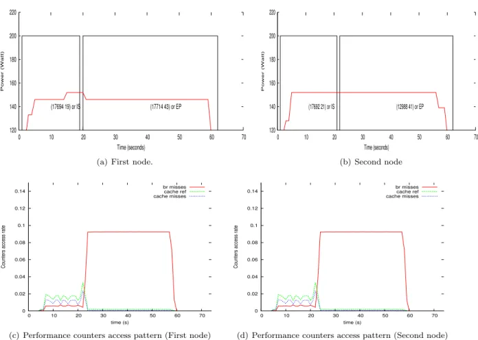
This example investigates how close to reality is our approach for partitioning a system’s runtime into different computational behaviours (or simply phases). To accomplish this, we successively run two appli-cations IS and EP from the NAS Parallel Benchmark (NPB) suite [21]. These appliappli-cations are opposite from their computational stand point in the sense that IS is communication intensive whereas EP is mainly computing. Data collected during their execution are used as input to the algorithm. Figure 1(b) and Figure 1(a) (where the curve gives the variation of the power consumption of the system over time and rectangles delimit detected phase) indicates that using a simple power model it is possible to detect phases the system when through. The couple of integers appearing in each rectangular on the figure gives for each phase the corresponding letter coded as an unsigned integer and the amount of time the system spent in that particular phase. For this example, the DNA-like structure of each node is straightforward, for the first node, it is: Idle(17694 19)(17714 43)Idle.
120 140 160 180 200 220 0 10 20 30 40 50 60 70 Power (Watt) Time (seconds) (17694 19) or IS (17714 43) or EP
(a) First node.
120 140 160 180 200 220 0 10 20 30 40 50 60 70 Power (Watt) Time (seconds) (17692 21) or IS (12988 41) or EP (b) Second node 0 0.02 0.04 0.06 0.08 0.1 0.12 0.14 0 10 20 30 40 50 60 70
Counters access rate
time (s)
br misses cache ref cache misses
(c) Performance counters access pattern (First node)
0 0.02 0.04 0.06 0.08 0.1 0.12 0.14 0 10 20 30 40 50 60 70
Counters access rate
time (s)
br misses cache ref cache misses
(d) Performance counters access pattern (Second node) Figure 1: Dividing NAS benchmarks IS and EP ran successively into two different computational behaviours using their power usage and sensors.
3.2. Execution vectors based system behaviour tracking
As it can be seen from Figure 1(c) and Figure 1(d) – where the y-axis represents the access rate of performance counters and the y-axis the execution time-line – that the access pattern of hardware perfor-mance counters or sensors in general strongly reflects changes in the behaviour of the application/system. We speak of sensors’ access rate because they are normalised with respect to the number of cycles. From the observation just made, the concept of execution vector which is similar to power vector (PV) [22] seems adequate for phase detection. An execution vector (EV) is defined as a column vector whose entries are system’s metrics, including hardware performance counters, network byte sent/received and disk read/write counts. To remain consistent with previous sections, we shall refer to these system metrics as sensors.
The sampling rate corresponding to the time interval after which sensors’ values are read depends on the granularity. While a larger sampling rate may hide information regarding the system’s behaviour, a smaller sampling rate may incur a non negligible overhead. In this paper, we use a sampling rate of one second and further normalize sensors with respect to the number of cycles to get their access rate.
We define the resemblance or similarity metric between two EVs as the manhattan distance between them. The Manhattan distance suits the case since it weighs more heavily differences.
A phase change is detected when the Manhattan distance between consecutive EVs exceeds a preset threshold. The threshold is fixed in the sense that it is always the same percentage – we refer to that percentage as the detection threshold – of the maximum distance between consecutive EVs (e.g., if the detection threshold is X%, then the threshold is X% of the maximum distance between consecutive EVs). however, the maximum distance between consecutive EVs is zeroed once a phase change is detected. So,
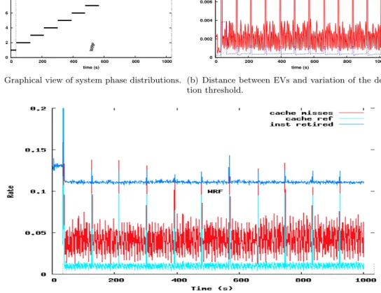
0 2 4 6 8 10 12 14 0 200 400 600 800 1000 phase id time (s) WRF
(a) Graphical view of system phase distributions.
0 0.002 0.004 0.006 0.008 0.01 0.012 0 200 400 600 800 1000 time (s) distance threshold
(b) Distance between EVs and variation of the detec-tion threshold.
(c) Cache reference and miss rates along with branch miss rate.
Figure 2: Phase changes detection using the similarity between consecutive execution vector as similarity metric.
technically, the threshold varies throughout the systems life cycle. The maximum existing distance between consecutive EVs is continuously updated until a phase change is detected where it is zeroed. The idea behind zeroing the maximum existing distance when a phase change occurs is to allow detecting phase changes when changing from a phase where distances between consecutive EVs are big to a phase where they are not and vice versa. For example, given a 10% similarity threshold, two consecutive EVs belong to the same group if the Manhattan distance between them is less than 10% of the maximum existing distance between all consecutive execution vectors. Figure 2(b) shows the distance between consecutive execution vectors and the variation of the threshold along the execution time-line when the system was running the Advance Research Weather Research and Forecasting (WRF-ARW) model [23]. A graphical view of our phase detection mechanism is provided in Figure 2(a), where dashed vertical lines indicate the start and end times of WRF-ARW. The left extremity of horizontal solid lines indicates the point (in the execution time-line) at which phase changes are detected and their length indicate the duration or length of corresponding phases. The x-axis represents the execution time-line and the y-axis represents IDs associated to detected phases. Note that IDs of phases are non zero integers ordered by their appearance order. It can be seen from Figure 2(c) that detected phases are corroborated by the access pattern of sensors.
The key motivation behind phase tracking is the use of characteristics of known phases for optimizing similar phases. Depending on the needs, optimizations aim to reduce the execution time of workloads, and/or their energy consumption. An effective phase characterization is therefore needed. To accomplish this, once a phase is detected, we apply principal component analyses (PCA) on the dataset composed of
EVs pertaining to that phase. We next select five sensors among those contributing the least to the first principal axis of PCA are kept for phase characterization. This choice is motivated by the assumption that information regarding what the system did not do during a phase is captured by sensors contributing the least to the first principal axis of PCA. These 5 sensors serve as the characteristic of the phase. Since data collected during a phase can be too large for efficient representation and comparison in hardware, we summarize a phase by the EV at the centroid of the group made up of EVs sampled during that phase. We refer to the EV summarizing a phase as the reference vector of that phase.
3.2.1. Partial Phase recognition.
Phase identification is an interesting property of phase detection mechanisms, since it allows reuse of system reconfiguration information for reoccurring phases. However, a phase cannot be identified with a known phase before its completion. The literature suggests using phase prediction, which predicts the next phase of an application before it gets started; however, it might not work very well when you don’t have any a priori information about applications sharing your platform. Therefore, instead of identifying a whole phase with a known, we propose to only identify a part of that phase with the known phase and extrapolate the result to the remaining part. We refer to that process as partial phase recognition; further details are provided in the next paragraph.
Partial phase recognition actually consists of identifying an ongoing phase (the phase has started and is
not yet finished) Pi with a known phase Pj only considering the already executed part of Pi. The already
executed part of Pi expressed as a percentage of the length (duration) of Pj is referred to as the recognition
threshold RT . Thus, with a RT % recognition threshold, and assuming that the reference vector of Pj is
EVPj and that its length is mj, an ongoing phase Piis identified with Pj if the manhattan distance between
EVPj and each EV pertaining to the already executed part of Pi (corresponding in length to RT % of mj)
are within the similarity threshold ST . The pseudo algorithm bellow summarises partial phase recognition.
• lets Pj be a completed phase, EVPj its reference vector, and mj its duration
• Pi is partially recognized as Pj if
– 8 v EV in the already executed part of Pi (that is, EVs sampled between the time stamp
corre-sponding to the start time of Piand the time stamp start time of Pi + RT % of mj), the distance
between v and EVPj is within threshold
4. Model use cases : system adaptation and energy consumption prediction
Understanding the different behaviours of a high performance computing (HPC) system goes through throughout its life cycle can lead to a multitude of optimization opportunities. In this section, we shall investigate how one can leverage those behaviours for reducing the energy consumption of its infrastructure. Platform as a service becoming more and more attractive users often face the dilemma of choosing between multiple platforms for their applications. This section also investigates how users can determine the least energy consuming platform for their applications. In the following, we first present show how our DNA-like modelling approach can be used for predicting the energy consumption of an application on a given platform. We next use our phase tracking methodology for reducing the energy consumption of applications without a priori knowledge.
4.1. Use case 1: cross platform energy prediction
The main motivation behind this use case is that users often have more than one candidate platform for running their jobs, in which case choosing the least energy consuming platform may be beneficial both for them and the platform provider. For simplicity, we assume that the application whose energy consumption is being predicted is the only application running on the platform under consideration. In other words, the DNA-like structure of the system at hand is that of the application.
The prediction model implicitly uses two sets of data, one from a reference platform provided by the DNA-like structure of the application, and one from a target platform which is the platform on which we want to estimate the overall energy consumption of the application. The aforementioned reference platform is the platform on which the application was first run and where its DNA-like structure was built. In most cases, the reference platform will be the platform on which the application was tested (nearly all the information – including the application’s energy consumption – in regard to the reference platform is known).
Knowing the DNA-like structure of an application, one can easily identify applications with the same computational requirements. We accomplish this by comparing the DNA-like structure of the ongoing application to known DNA-like structures. A match is found when the already executed part of the ongoing application matches with a given percentage of the known DNA-like structure.
Let’s denote Etar the energy consumed by the already executed part of the application of which we
want to estimate the energy consumption and Eref the energy consumed by the corresponding part of
the application whose DNA-like matches with the already executed part of the application at hand (the application that we want to estimate the energy consumption). For example, considering an application
that lasts 60 minutes on its reference platform, let’s assume that Etar represents the energy consumed by
the same application on the target platform after 10 minutes run; therefore, Eref represents the proportion
of energy consumed by the application on the reference platform during the first 10 minutes of its execution.
Denoted as Erel, the relative energy consumption between the two platforms is given by the following
equation:
Erel=
Etar
Eref
(1) With the above relative energy, the estimated energy consumption of the application on the target platform is given by Equation 2:
Eest= Z X% 0 P(t)i,tardt+ Erel⇤ Z end X% P0(t) j,refdt (2)
Where Eest is the estimated energy consumption on the target platform; Erel the relative energy
con-sumption between the target platform and the reference platform. In the above equation,R0X%P(t)i,tardt
represents the energy consumed by the application before a match is found with a known DNA-like structure.
Either measured or estimated, P (t)i,tar is the instantaneous power usage of the application on the target
platform. Likewise, P0(t)
j,ref is the instantaneous power usage of the application on the reference platform
and can be obtained from its DNA-like structure. In cases where the power consumption may radically change after the X% threshold, if the change in power consumption does not imply any change in the set of sensors used to estimate the power consumption, then we still assume it is the same application otherwise we attempt to find another match.
We define the estimation accuracy as the ratio between estimated and measured energy on the target platform, i.e,
Accuracy= Eest tar
Etar
(3)
where Eest tar is the estimated energy consumption on the target platform.
Although comparing two DNA-lire structures boils down to comparing two strings, the overhead associ-ated with matching the DNA-like structure of a running application with previously seen known applications is proportional to the size of already known applications times the size of the DNA-like structure of the running application. We simplify this with the assumption that our profile database only contains one application which is that of the application of which we want to predict the energy consumption. We also assume that the application follow a very simple pattern which starts with an initialization phase and finishes which a finalization phase. Between the initialization and the finalization phases, there are some iterative computations and optional communications. Finally, assuming that the instantaneous power usage of the application is approximately the same during each of its iterations; meaning that the energy consumed by
the application in each iteration throughout its life cycle is nearly the same, Equation 2 can be simplified to
Equation 4; where Einit represents the energy consumed by the application on the target platform during
its initialization phase; Eref −init is the energy consumed by the application on the reference platform from
the end of the initialization phase to the end of its whole execution; and Eref −exe is the measured energy
consumption (resulting from complete execution) of the application on the reference platform.
Eest= Einit+ Erel⇤ (Eref −exe− Eref −init) (4)
4.2. Use case 2: optimizing energy performance of HPC systems
The methodology described in Section 3.2 permits online detection and characterisation of different runtime behaviours of the system. We use the coupling with partial phase recognition to guide on-the-fly system adaptation considering three HPC subsystems: processor, disk and network interconnect. The power consumption of these HPC subsystems along with that of the memory is about 55% [24] of the total power consumption of a typical HPC system. For the processor, we define three computational levels according to the characteristics of the workload:
• high or cpu-bound: the cpu-bound computational level corresponds to the maximum available CPU frequency, and is used for CPU-bound workloads
• medium or memory-bound: corresponds to an average in between the maximum and the minimum available frequencies; it is mainly used for memory-bound workloads.
• low: the system is in the low computational level when the CPU frequency is set to the minimum available.
For the disk, we define two states: active and sleep; where active includes both the disk’s active and standby modes. Finally, for the network interconnect we define two data transfer speeds:
• the communication-intensive speed: corresponds to the highest available transfer rate of the network card.
• low-communication speed: where the speed of the network interconnect is set to the lowest speed. As mentioned earlier in this paper, principal component analysis (PCA) is applied to vectors belonging to any newly created phase for selecting five sensors which are used as phase characteristics. These charac-teristics are translated into system adaptation as detailed in Table 2. Let’s comment the first line of that table. Workloads/applications with frequent cache references and misses are likely to be memory bound. In our case, having these sensors (cache reference and cache misses) selected from PCA indicates that the workload is not memory bound. If in addition that workload does not issue a high I/O rate (presence of I/O related sensors in the first column), then we assume that it is CPU-bound; consequently, the frequency of the processor can be scaled to its maximum, the disk sent to sleep and the the speed of the interconnect scaled down. For the second line of Table 2, the characteristics do not include any I/O related sensor, this implies that the system was running and I/O intensive workload; thus, the processor’s speed can be set to its minimum. Note in passing that changing the disk’s state from sleep to active does not appear in Table 2, this is because the disk automatically enters the active state when it is accessed.
5. Experimentation and validation
5.1. Evaluation for energy consumption prediction
We evaluate our energy estimation model considering two workloads: the first workload (workload 1 ) iteratively computes the the inverse of a 10x10 matrix and copies a large file from a remote repository; the second workload we attempt to estimate the energy consumption is GeneHunter [25].
We further consider three scenarios: (i) the first scenario estimates the energy consumption of workload 1 on a node running at 2.13GHz using the same node running at 1.6GHz as the reference platform; (ii) scenario
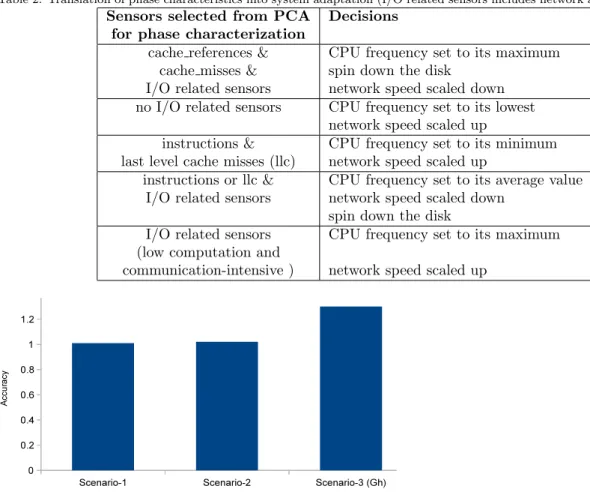
Table 2: Translation of phase characteristics into system adaptation (I/O related sensors includes network and disk activities).
Sensors selected from PCA Decisions
for phase characterization
cache references & CPU frequency set to its maximum
cache misses & spin down the disk
I/O related sensors network speed scaled down
no I/O related sensors CPU frequency set to its lowest
network speed scaled up
instructions & CPU frequency set to its minimum
last level cache misses (llc) network speed scaled up
instructions or llc & CPU frequency set to its average value
I/O related sensors network speed scaled down
spin down the disk
I/O related sensors CPU frequency set to its maximum
(low computation and
communication-intensive ) network speed scaled up
Figure 3: Per scenario energy estimation accuracy.
2 still estimate the energy usage of workload 1 but uses Dell Power Edge server and the target platform is a Sun Fire V20z as reference and target platforms respectively; (iii) in the third and last scenario we attempt to estimate the energy consumption of GeneHunter. For this specific case, our reference platform is an Intel Xeon E5506 Quad-core with 8 cores and 12GB of RAM while the target platform is an an Intel Xeon X3440 with 4 cores and 16GB of RAM. For all three scenarios, an empiric partial execution threshold of 20% is used. This means that, a match with an existing DNA-like structure DS is found if the already executed part of our synthetic application matches with 20% of DS, i.e., assuming DS lasted 60 seconds, a match will be found if the already executed part of the synthetic application matches with the DNA-like structure describing the first 12 seconds of DS.
We compute for each scenario the expected energy consumption based on Equations 4; results are summarized in Figure 3. We can see from those results that the accuracy is very good. Notice that the accuracy is higher because it is computed considering the average energy consumption. We believe that overestimating the actual energy consumption (as Figure 3 indicates) is acceptable since the peak energy consumption is typically greater than the average. We can also notice that the accuracy for Gene Hunter is extremely high, this can be attributed to the fact that we were unable to divide the application into phases reflecting its actual behaviour.
5.2. Execution vectors based system behaviour tracking guided system adaptation
In this section, we analyse and discuss experimental results for our energy performance optimization use case.
5.2.1. Evaluation platform
Our evaluation support is a twenty five node cluster set up on the Grid5000 [26] french large scale experimental platform. Each node is an Intel Xeon X3440 with 4 cores and 16 GB of RAM. Available frequency steps for each core are: 2.53 GHz, 2.40 GHz, 2.27 GHz, 2.13 GHz, 2.00 GHz, 1.87 GHz, 1.73 GHz, 1.60 GHz, 1.47 GHz, 1.33 GHz and 1.20 GHz. In our experiments, low computational level always sets the CPU frequency to the lowest available which is 1.20 GHz, whereas high and medium computational levels set the CPU frequency to the highest available (2.53 GHz) and 2.00 GHz respectively. Each node uses its own hard drive which supports active, ready and standby states. Infiniband-20G is used for interconnecting nodes. The Linux kernel 2.6.35 is installed on each node where perf event is used to read the hardware monitoring counters. MPICH is used as MPI library. For the experiments, we use three benchmarks (LU, BT and SP) from NPB suite and two real-life applications: Molecular Dynamics Simulation (MDS) [27] and the Advance Research Weather Research and Forecasting (WRF-ARW) model [28, 23]. WRF-ARW is a fully compressible conservative-form non-hydrostatic atmospheric model. It uses an explicit time-splitting integration technique to efficiently integrate the Euler equation. The classical Molecular Dynamics solves numerical Newton’s equations of motion for the interaction of the many particles system. We monitored each node’s power usage with one sample per second using a power distribution unit.
5.2.2. Results analyses and discussion.
To evaluate our system adaptation policy, we consider 3 basic configurations of the monitored cluster: the first configuration which we refer to as demand is the configuration in which the default linux’s on-demand governor is enabled on all the nodes of the cluster; the second configuration called performance is the configuration in which the linux’s performance governor is enabled on each node of the cluster; and finally the third configuration which we refer to as managed is the configuration in which our system adaptation policy is applied. We also consider two levels of system adaptation:
• system adaptation level one: It corresponds to the situation in which only processor related optimiza-tion is made
• system adaptation level two: It embraces level one, and additionally considers optimizing the inter-connect and the disk.
Results we present here are obtained using an empirical similarity threshold ST of 5%. The same goes for the recognition threshold RT which is set to 10%.
(a) System adaptation level one: Processor’s only optimization: when an ongoing phase is identified
with an existing phase, the characteristics of the existing phase are used to adapt the processor’s frequency accordingly. Diagrams of Figure 4 show the average energy consumption (Figure 4(a)) and execution time (Figure 4(b)) of MDS and WRF-AWR under the three system’s configurations. These diagrams indicate that our management policy can save up to 19% of the total energy consumption with less than 4% performance loss.
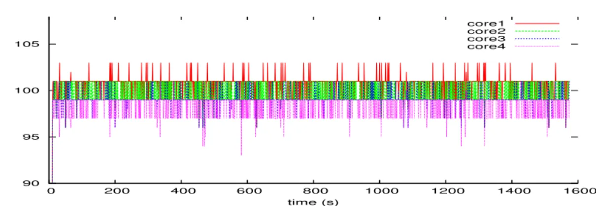
Figure 4(b) shows that on-demand and performance governors nearly achieve the same performance. This is because linux’s on-demand governor do not lower the CPU frequency unless the system load decreases below a given threshold. Traces of CPU load under WRF-AWR for one node of our cluster are shown in Figure 5, where the y-axis represents the percentage of load. The plot indicates that the CPU load remains above 85%, in which case the on-demand and performance governors almost have the same behaviour. With processor’s only optimization, our management policy differs from that of the linux’s on-demand governor in that we do not use the system’s load as system adaptation metric, which enable us to consume less energy.
(b) System adaptation level two: Processor, disk and network optimization: Figure 6 presents the energy
performance considering the processor, along with disk and network. These graphs indicate that considering the processor along with disk and network interconnect improves energy performance up to 24% with the same performance degradation as with processor’s only optimization. In other words, the disk and the network also contribute in improving energy performance.
0 % 20 % 40 % 60 % 80 % 100 % MDS WRF-ARW
Normalized energy consumption
performance managed on-demand
(a) Average energy consumed by each application under different configurations. 0 % 20 % 40 % 60 % 80 % 100 % MDS WRF-ARW
Normalized execution time
(b) Average execution time of each application under differ-ent configurations
Figure 4: Phase tracking and partial recognition guided CPU optimization results
90 95 100 105
0 200 400 600 800 1000 1200 1400 1600
load per core
time (s)
core1 core2 core3 core4
Figure 5: Load traces for one of the nodes running WRF-AWR under the on-demand configuration.
0 % 20 % 40 % 60 % 80 % 100 % MDS WRF-ARW
Normalized energy consumption
performance managed on-demand
(a) Energy performance.
0 % 20 % 40 % 60 % 80 % 100 % MDS WRF-ARW
Normalized execution time
(b) Performance (execution time)
Figure 6: Phase tracking and partial recognition guided processor, disk and network interconnect optimization results: the chart shows average energy consumed by each application under different configurations.
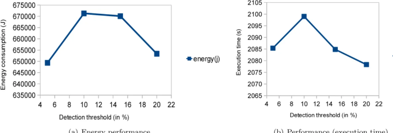
(a) Energy performance. (b) Performance (execution time) Figure 7: Impact of the detection threshold on energy performance for WRF-AWR.
(a) Energy performance. (b) Performance (execution time)
Figure 8: Influence of the partial recognition threshold on energy performance for WRF-AWR.
5.2.3. Threshold selection and energy performance
In this section, we investigate the influence of phase detection parameters ST and RT on application performance and energy consumption. Firstly, we set the detection threshold and vary the partial recognition threshold. Secondly, we set the partial recognition threshold and vary the detection threshold. Figure 7 where the x-axis represents the average energy consumption and the y-axis the detection threshold shows the impact of the detections threshold both on execution time and energy performance of WRF-AWR. It can be seen from that figure that for WRF-AWR, a detection threshold either of 5% or 20% could be a good choice. However, 5% could be preferable since there is a difference in energy consumption of up to 5000 Joules, for a less than 10 seconds difference in execution time. Figure 7 also reveals that the detection threshold might have a significant impact on performance (both in terms of energy consumption and execution time). For these experiments, the partial recognition threshold was fixed to 10%.
The influence of the recognition threshold RT on energy performance is summarised by Figure 8, where the x-axis represents the recognition threshold and the y-axis the average energy consume by the application under different partial recognition threshold settings. According to Figure 8, a partial recognition threshold of 15% is convenient both in terms of energy and execution time.
What we can learn from Figure 7 and Figure 8 is that these values must be chosen depending on the target objective. A small recognition threshold may limit the impact of wrong decisions; however it may also have an influence on right decisions. For, making the right decision earlier allows saving more energy, in reverse, making a wrong decision earlier can result in significant energy waste and/or performance degradation.
Figure 9: Energy and performance (execution time) when BT and WRF-AWR are sharing the cluster.
5.3. Performance analyses of multiple applications
Earlier herein, we talked about the usefulness to look at a whole system; however, our evaluations has so far focused on only one application at a time. In this section, we evaluate our strategy with multiple applications running at the same time. We consider as test applications the WRF-AWR model and BT from the NAS Parallel Benchmark (NPB) suite. WRF-AWR spans 48 processes and run on 48 cores (in other words 12 nodes) whereas BT spans 48 processes on 12 nodes. The two applications do not share any resources except the network that interconnect them. We measure the power consumption of each of our 24-node cluster using a power distribution unit (PDU). Figure 9, where the x-axis represents the average percentage of energy improvement or performance loss, indicates that our methodology still function when there multiple applications sharing the platform; however, we also notice a performance degradation of up to 15% for BT. We are currently investigating the reason of BT performance degradation. Nevertheless, we believe this can be attributed to the fact that some phases might have been considered as memory intensive or communication intensive while they were actually compute intensive. In addition, applications (BT for example) which do not implement load imbalance are likely to experience higher performance degradation than those which implement load imbalance (WRF-AWR for example) [29, 30].
6. Conclusion and future works
In this paper, we present two generic approaches for tracking high performance computing systems’ be-haviour regardless of the applications being executed. We show through two use cases how they can be used for improving energy performance of a HPC system at runtime in one hand and in another hand how they can be used for estimating the energy consumption of an application given a target platform. Experimental results reveal the effectiveness of these two methodologies under real-life workloads and benchmarks. Com-parison of our system adaptation policy with baseline unmanaged execution shows that we can save up to 19% of energy with less than 4% performance loss considering the processor only and up to 24% considering the disk, processor and network. As our methodology for improving energy performance does not depend on any application specific metric, we expect it to be extended to a large number of power-aware HPC systems. Future works include combining the two system’s behaviour tracking to enable live feedback on whether a system adaptation will be effective or not. This can help improving the energy performance while reducing performance loss. We also plan on adding memory optimization to processor, disk and network optimiza-tion and integrating workload consolidaoptimiza-tion and migraoptimiza-tion as core funcoptimiza-tionalities of the system management policy.
Acknowledgment
This work is supported by the INRIA large scale initiative Hemera focused on ”developing large scale par-allel and distributed experiments”. Experiments presented in this paper were carried out using the Grid’5000 experimental testbed, being developed under the INRIA ALADDIN development action with support from CNRS, RENATER and several Universities as well as other funding bodies (see https://www.grid5000.fr). References
[1] NVDIA, Nvidia tesla gpus power world’s fastest supercomputer, Press Release, 2010.
[2] INTEL, Developer’s manual: Intel 80200 processor based on intel xscale microarchitecture, 1998. [3] AMD, Mobile amd duron processor model 7 data sheet, 2001.
[4] G. L. T. Chetsa, L. Lef`evre, J.-M. Pierson, P. Stolf, G. D. Costa, Dna-inspired scheme for building the energy profile of
hpc systems, in: E2DC, volume 7396 of Lecture Notes in Computer Science, Springer, 2012, pp. 141–152.
[5] G. L. Tsafack, L. Lefevre, J.-M. Pierson, P. Stolf, G. Da Costa, Beyond cpu frequency scaling for a fine-grained energy control of hpc systems, in: SBAC-PAD 2012 : 24th International Symposium on Computer Architecture and High Performance Computing, IEEE, New York City, USA, 2012, pp. 132–138.
[6] G. D. Costa, H. Hlavacs, Methodology of measurement for energy consumption of applications, in: GRID, IEEE, 2010, pp. 290–297.
[7] I. Kadayif, T. Chinoda, M. Kandemir, N. Vijaykirsnan, M. J. Irwin, A. Sivasubramaniam, vec: virtual energy counters, in: Proceedings of the 2001 ACM SIGPLAN-SIGSOFT workshop on Program analysis for software tools and engineering, PASTE ’01, ACM, New York, NY, USA, 2001, pp. 28–31.
[8] G. Contreras, Power prediction for intel xscale processors using performance monitoring unit events, in: In Proceedings of the International symposium on Low power electronics and design (ISLPED, ACM Press, 2005, pp. 221–226.
[9] K. Singh, M. Bhadauria, S. A. McKee, Real time power estimation and thread scheduling via performance counters, SIGARCH Comput. Archit. News 37 (2009) 46–55.
[10] D. Bautista, J. Sahuquillo, H. Hassan, S. Petit, J. Duato, A simple power-aware scheduling for multicore systems when running real-time applications, in: IPDPS, IEEE, 2008, pp. 1–7.
[11] R. Joseph, M. Martonosi, Run-time power estimation in high performance microprocessors, in: In International Symposium on Low Power Electronics and Design, pp. 135–140.
[12] W. Wu, L. Jin, J. Yang, P. Liu, S. X. D. Tan, A systematic method for functional unit power estimation in microprocessors, in: Design Automation Conference.
[13] SUN, The ultrasparc processor - technology white paper: The ultrasparc architecture, 1995.
[14] INTEL, Intel xscale microarchitecture for the pxa255 processor: User’s manual intel corporation, 2003.
[15] B. Rountree, D. K. Lownenthal, B. R. de Supinski, M. Schulz, V. W. Freeh, T. Bletsch, Adagio: making dvs practical for complex hpc applications, in: Proceedings of the 23rd international conference on Supercomputing, ICS ’09, ACM, New York, NY, USA, 2009, pp. 460–469.
[16] V. W. Freeh, N. Kappiah, D. K. Lowenthal, T. K. Bletsch, Just-in-time dynamic voltage scaling: Exploiting inter-node slack to save energy in mpi programs, J. Parallel Distrib. Comput. 68 (2008) 1175–1185.
[17] R. Kotla, A. Devgan, S. Ghiasi, T. Keller, F. Rawson, Characterizing the impact of different memory-intensity levels, in: In IEEE 7th Annual Workshop on Workload Characterization (WWC-7.
[18] C. Isci, G. Contreras, M. Martonosi, Live, runtime phase monitoring and prediction on real systems with application to dynamic power management, in: Proceedings of the 39th Annual IEEE/ACM International Symposium on Microarchi-tecture, MICRO 39, IEEE Computer Society, Washington, DC, USA, 2006, pp. 359–370.
[19] K. Choi, R. Soma, M. Pedram, Fine-grained dynamic voltage and frequency scaling for precise energy and performance tradeoff based on the ratio of off-chip access to on-chip computation times, Trans. Comp.-Aided Des. Integ. Cir. Sys. 24 (2006) 18–28.
[20] M. Y. Lim, V. W. Freeh, D. K. Lowenthal, Adaptive, transparent frequency and voltage scaling of communication phases in mpi programs, in: Proceedings of the 2006 ACM/IEEE conference on Supercomputing, SC ’06, ACM, New York, NY, USA, 2006.
[21] D. H. Bailey, E. Barszcz, J. T. Barton, D. S. Browning, R. L. Carter, R. A. Fatoohi, P. O. Frederickson, T. A. Lasinski, H. D. Simon, V. Venkatakrishnan, S. K. Weeratunga, The nas parallel benchmarks, Technical Report, The International Journal of Supercomputer Applications, 1991.
[22] C. Isci, M. Martonosi, Identifying program power phase behavior using power vectors, in: In Workshop on Workload Characterization.
[23] W. C. Skamarock, J. B. Klemp, J. Dudhia, D. O. Gill, D. M. Barker, W. Wang, J. G. Powers, A description of the advanced research wrf version 2, AVAILABLE FROM NCAR; P.O. BOX 3000; BOULDER, CO 88 (2001) 7–25. [24] Y. Liu, H. Zhu, A survey of the research on power management techniques for high-performance systems, Softw. Pract.
Exper. 40 (2010) 943–964.
[25] G. Conant, S. Plimpton, W. Old, A. Wagner, P. Fain, Parallel genehunter: Implementation of a linkage analysis package for distributed-memory architectures, in: In Proceedings of the First IEEE Workshop on High Performance Computational Biology, International Parallel and Distributed Computing Symposium, p. electronic.
[26] R. Bolze, F. Cappello, E. Caron, M. Dayd´e, F. Desprez, E. Jeannot, Y. J´egou, S. Lanteri, J. Leduc, N. Melab, G. Mornet, R. Namyst, P. Primet, B. Quetier, O. Richard, E.-G. Talbi, I. Touche, Grid’5000: A large scale and highly reconfigurable experimental grid testbed, Int. J. High Perform. Comput. Appl. 20 (2006) 481–494.
[27] K. Binder, J. Horbach, W. Kob, W. Paul, F. Varnik, Molecular dynamics simulations, Journal of Physics: Condensed Matter 16 (2004) S429.
[28] WRF-AWR, The weather research and forecasting mode, 2012.
[29] G. Chen, K. Malkowski, M. T. Kandemir, P. Raghavan, Reducing power with performance constraints for parallel sparse applications, in: IPDPS, IEEE Computer Society, 2005.
[30] H. Kimura, M. Sato, Y. Hotta, T. Boku, D. Takahashi, Emprical study on reducing energy of parallel programs using slack reclamation by dvfs in a power-scalable high performance cluster, in: CLUSTER, IEEE, 2006.