Cellular Skeletons: a New Approach to Topological Skeletons with Geometric Features

HAL Id: hal-01341037

https://hal-amu.archives-ouvertes.fr/hal-01341037

Submitted on 23 Feb 2017

HAL is a multi-disciplinary open access

archive for the deposit and dissemination of

sci-entific research documents, whether they are

pub-lished or not. The documents may come from

teaching and research institutions in France or

abroad, or from public or private research centers.

L’archive ouverte pluridisciplinaire HAL, est

destinée au dépôt et à la diffusion de documents

scientifiques de niveau recherche, publiés ou non,

émanant des établissements d’enseignement et de

recherche français ou étrangers, des laboratoires

publics ou privés.

Cellular Skeletons: a New Approach to Topological

Skeletons with Geometric Features

Aldo Gonzalez-Lorenzo, Alexandra Bac, Jean-Luc Mari, Pedro Real

To cite this version:

Aldo Gonzalez-Lorenzo, Alexandra Bac, Jean-Luc Mari, Pedro Real. Cellular Skeletons: a New

Ap-proach to Topological Skeletons with Geometric Features. 16th International Conference on Computer

Analysis of Images and Patterns (CAIP 2015), Sep 2015, La Valette, Malta. pp.616-627,

�10.1007/978-3-319-23117-4_53�. �hal-01341037�

Cellular Skeletons:

a New Approach to Topological Skeletons

with Geometric Features

Aldo Gonzalez-Lorenzo1,2_{, Alexandra Bac}1_{, Jean-Luc Mari}1_{, and Pedro Real}2

1 _{Aix-Marseille Universit´e, CNRS, LSIS UMR 7296,13397, Marseille (France)}

2

University of Seville, Institute of Mathematics IMUS, Seville (Spain)

Abstract. This paper introduces a new kind of skeleton for binary vol-umes called the cellular skeleton. This skeleton is not a subset of voxels of a volume nor a subcomplex of a cubical complex: it is a chain complex together with a reduction from the original complex.

Starting from the binary volume we build a cubical complex which rep-resents it regarding 6 or 26-connectivity. Then the complex is thinned using the proposed method based on elementary collapses, which pre-serves significant geometric features. The final step reduces the number of cells using Discrete Morse Theory. The resulting skeleton is a reduction which preserves the homology of the original complex and the geometri-cal information of the output of the previous step.

The result of this method, besides its skeletonization content, can be used for computing the homology of the original complex, which usually provides well shaped homology generators.

1

Introduction

The notion of skeleton (or medial axis) was introduced by H. Blum in 1967 [Blu67]. Given a subset S ⊂ Rn_{, its medial axis is the set of all the points in S}

that are centres of maximal balls included in S. It is a good descriptor of shape, it is thin, it has the same type of homotopy as S (one can be continuously deformed into the other) and it is reversible (we can reconstruct S by using the distance of each point to the boundary).

Skeletons are widely used for various applications such as video tracking [GSdA+09], shape recognition [YWZ08], surface sketching [Mar09] and in many other scientific domains.

In the discrete context there is no unique equivalent to the continuous defini-tion. A discrete medial axis gives a skeleton which is not homotopically equivalent to the discrete object. Discrete skeletons are usually based on the thinning of the object, using mathematical morphology or parallel approaches: simple points [KR89], simple P-points [LB07], critical kernels [CB14]. The given skeleton is a subset of voxels, much smaller, which is homotopically equivalent and should pre-serve in an uncertain way the geometrical features of the object. There is another class of skeletons which first computes a cubical complex associated to an ob-ject and then selects a subcomplex (see [CC09, LCLJ10, Cou11, Cou13, DS14]).

We must note that geometrical preservation is more intuitive or heuristic in the context of discrete skeletons than in the continuous one. Hence, all previous approaches exist, with their respective strengths and weaknesses.

This paper presents a three-step method:

1. Starting from a binary volume (a set of voxels in a regular grid), we define its associated cubical complex. We propose two different constructions which encode 6 and 26-connectivity. These associated cubical complexes were sep-arately defined in [CC09, LCLJ10]

2. We compute a skeleton of this cubical complex. We propose a method strongly based on [LCLJ10] which performs elementary collapses which are encoded in a discrete gradient vector field (DGVF). It is a simple algorithm producing satisfying results. This step can also be addressed with the algorithms found in [LCLJ10, DS14] or in [CC09, Cou11, Cou13] given a fixed parameter. As a result, the shape of the skeleton is defined

3. This step is completely new. Given the reduced cubical complex, we extend the previous DGVF in order to obtain a reduction (see [Ser92]) between the chain complex of the original cubical complex and a reduced one, with the property of maintaining the shape of the skeleton computed in the second step.

Our approach presents several advantages: the topology preservation through-out the thinning is guaranteed by the Discrete Morse Theory; our method disso-ciates connectivity and skeleton extraction, thus the thinning algorithm becomes independent of the connectivity relation; the obtained reduction accelerates the computation of its homology since the reduced complex contains fewer cells. Moreover, starting the homology computation from this cellular skeleton should produce well shaped homology generators, as they are included in the skeleton. This reveals an advantage of computing homology using Discrete Morse Theory: we can control the shape of the homology generators.

In Sect. 2, we introduce all the necessary definitions for understanding our method. In Sect. 3, we describe our approach. Section 4 shows some results of our framework on some binary volumes. We finish this paper by presenting our conclusion and our future perspectives.

2

Preliminaries

2.1 Binary Volumes and Cubical Complexes

A 3D binary volume is a set of voxels centred on integer coordinates. We will describe it by the set of the coordinates of its elements.

The rest of this section is derived from [KMM04]. For a deeper understanding of these concepts, the reader can refer to it. An elementary interval is an interval of the form [k, k+1] (nondegenerate) or a set {k} (degenerate), also denoted as [k, k], where k ∈ Z. An elementary cube in Rn _{is the Cartesian product of n}

is its dimension. An elementary cube of dimension q will be called q-cube for short, or even q-cell, since cubical complexes are a special kind of cell complexes. Given two elementary cubes P and Q, we say that P is a face of Q if P ⊂ Q and we note it P < Q. It is a primary face if the difference of their dimensions is 1. The definitions of the dual concepts coface and primary coface are immediate. A cubical complex is a set of elementary cubes with all of their faces. The boundary of an elementary cube is the collection of its primary faces.

A cubical complex can be completely described by its Hasse diagram. It is a directed graph whose vertices are all the elementary cubes, and whose arrows go from each cube to its primary faces. In this paper we will usually not make the distinction between the vertices and the elementary cubes they represent, so we will mix the terms vertex, cube and cell.

2.2 Chain Complexes

A chain complex (C∗, d∗) is a sequence of R-modules C0, C1, . . . (called chain

groups) and homomorphisms d1: C1→ C0, d2: C2→ C1, . . . (called differential

or boundary operators) such that dq−1dq = 0, ∀q > 0, where R is some ring,

called the ground ring or ring of coefficients.

Given a cubical complex, we define its chain complex (with coefficients in Z2) as follows:

– Cq is the free group generated by the q-cubes of the complex. Their elements

are called q-chains.

– dq gives the “algebraic” boundary, which is the sum of the primary faces of

the q-cubes.

2.3 Discrete Morse Theory

Discrete Morse Theory was introduced by Robin Forman as a discretization of the Morse Theory [For02]. The main idea is to obtain some homological informa-tion by means of a funcinforma-tion defined on the complex. This funcinforma-tion is equivalent to a discrete gradient vector field and we will rather use this notion.

A discrete vector field on a cubical complex is a matching on its Hasse di-agram, that is a collection of edges such that no two of them have a vertex in common. From a Hasse diagram and a discrete vector field we can define a Morse graph: it is a graph similar to the Hasse diagram except for the arrows contained in the matching, which are reverted. These arrows will be called integral arrows, and the others, differential arrows.

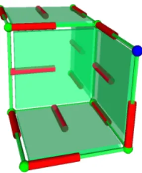
A V-path is a path on the Morse graph which alternates between integral and differential arrows. A discrete gradient vector field is a discrete vector field which does not contain any closed V-path. A critical vertex (or critical cell) is a vertex which is not paired by the matching. Figure 1 shows a cubical complex with a DGVF.

A DGVF can be given by a set of elementary collapses. An elementary col-lapse [Whi50] consist of removing a free pair from a cell complex, that is a cell

Fig. 1: A DGVF over a cubical complex. Red segments represent integral ar-rows going from one cell to some of its primary cofaces. The critical cells are represented in blue.

with a primary face which does not have any other coface. A collapse is a se-quence of elementary collapses. The homotopy type of a complex is invariant under collapses. The free pairs of a collapse define a DGVF.

2.4 Reduction

The Effective Homology theory [Ser92] provides a tool that establishes a strong relation between two chain complexes, called reduction. Formally, a reduction between two chain complexes (C∗, d∗) and (C∗0, d0∗) is a triple of homomorphisms

(h∗, f∗, g∗) such that:

– hq : Cq → Cq+1 for every q ≥ 0

– fq : Cq→ Cq0 is a chain map (f d = d0f )

– gq: Cq0 → Cq is also a chain map (gd0= dg)

– gf = 1 − dh − hd – f g = 1C0

– hh = hf = hg = 0

This notion is a special case of chain contraction [EL53] or strong deformation retraction data [LS87]. It is a usual tool for reducing chain complexes in order to compute their homology. We will use it to define the Morse complex of a cubical complex endowed with a DGVF. The exact definition is given in [GBMR14]. Roughly speaking, the Morse complex is a cell complex composed of the critical cells, which is homotopically equivalent to the original cubical complex.

3

Our Framework

In this section we present the structure of our framework. It should be noted that, although the algorithms are designed for 3D volumes, they can be generalized to any dimension: one only needs to replace parameter 3 by n.

Let us briefly recall the structure of our approach, previously described in the introduction. We start with a binary 3D volume. Depending of the connectivity relation which we want to use (6 or 26), we build its associated cubical complex with one of the methods explained in Sect. 3.2. Next, we make a homotopic thin-ning of the cubical complex based on elementary collapses encoded in a DGVF. Finally we minimize the number of cells in the Morse complex by preserving its shape in Algorithm 4.

The final result is a cellular skeleton: a reduction from the original complex to a reduced one. Then we give a representation of this skeleton by showing the cells of the chain f (σ) (see Sect. 2.4) for every critical cell.

3.2 Construction of the Cubical Complex: Choosing the Connectivity

As explained earlier, the first step of our approach consists in building the cubical complex associated to the digital volume and the connectivity relation chosen. Hence, there are two encodings: one for 6-connectivity (that is 2n-connectivity in dimension n) and other for 26-connectivity ((3n_{− 1)-connectivity). Figure 2}

illustrates these two cubical complexes associated to the same binary volume.

Fig. 2: Left: a binary volume. Center: its primal associated cubical complex. Right: its dual cubical complex

The primal associated cubical complex. We encode a binary volume equipped with 26-connectivity into a cubical complex (called primal associated cubical complex ). In this case, the construction is quite elementary as every voxel x = (x1, x2, x3) generates the 3-cube [x1, x1+ 1] × [x2, x2+ 1] × [x3, x3+ 1] and all

its faces. This method was already presented in [CC09].

The dual associated cubical complex. Another approach consists in en-coding a binary volume equipped with 6-connectivity into a cubical complex (called dual associated cubical complex ). Let us first adapt the notion of clique to our context: a d-clique is a maximal (in the sense of inclusion) set of voxels such that their intersection is a d-cube. First, for every voxel (in fact 3-clique) x = (x1, x2, x3) of the volume, we add the 0-cube σ = [x1] × [x2] × [x3]. Then, for

every d-clique (d < 3) in the volume, we add to the cubical complex a (3 − d)-cube such that its vertices are the voxels of the d-clique. This approach was used in [LCLJ10].

3.3 Homotopic Thinning Algorithm

This step performs a homotopic thinning of the cubical complex. This is done by establishing a DGVF, which can be seen as a set of elementary collapses (deletion of free pairs). Actually, this DGVF describes the relation between the original complex and the thinned one (the Morse complex) in terms of a reduction. Let us point out that our approach does not have to deal with simple points, critical kernels, etc.

A simple thinning algorithm with satisfying results was given in [LCLJ10]. The algorithm is described in three steps:

Step 1: Thinning Perform an iterative thinning: at each iteration, all free pairs are identified and then collapsed while it is possible. For every cell σ, I(σ) is the first iteration after which σ has no cofaces and R(σ) is the iteration in which σ is removed. If I(σ) is defined,

Mabs(σ) = R(σ) − I(σ) and Mrel(σ) = 1 −

I(σ) R(σ)

Step 2: Clustering Given some thresholds εq_abs, εq_reland τq(k = 1, 2), consider the set B of the cells scoring higher than εq_abs and εq_rel. Remove from this set those cells whose connected component size is fewer than τq.

Step 3: Thinning Repeat the first step while maintaining the cells in B.

Note that when we identify all the free pairs, we can find several pairs (τ > σ1), (τ > σ2), . . . and we must choose one of them. This choice was defined

as arbitrary in [LCLJ10] and it was pointed out that this should be studied. Our contribution in this step is an alternative to the simple iterative collapse which makes some of these collapses order-independent. It is described in detail in Algorithm 2, which calls Algorithm 1.

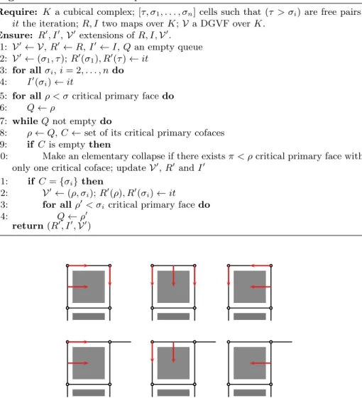
Indeed, for each elementary collapse between a maximal cell τ and one of its primary faces σ1, . . . , σn, we must choose one of them. We partially solve this

problem by performing multiple elementary collapses (see Algorithm 1) in the same iteration in order to remove some of these cells. Sometimes the choice of the cell σ1is irrelevant, as shown in Fig. 3. This seems to be related to the notion

Algorithm 1 AdvancedCollapse

Require: K a cubical complex; [τ, σ1, . . . , σn] cells such that (τ > σi) are free pairs;

it the iteration; R, I two maps over K; V a DGVF over K. Ensure: R0, I0, V0extensions of R, I, V0.

1: V0← V, R0_{← R, I}0_{← I, Q an empty queue}

2: V0← (σ1, τ ); R0(σ1), R0(τ ) ← it

3: for all σi, i = 2, . . . , n do

4: I0(σi) ← it

5: for all ρ < σ critical primary face do

6: Q ← ρ

7: while Q not empty do

8: ρ ← Q, C ← set of its critical primary cofaces

9: if C is empty then

10: Make an elementary collapse if there exists π < ρ critical primary face with

only one critical coface; update V0, R0 and I0

11: if C = {σi} then

12: V0← (ρ, σi); R0(ρ), R0(σi) ← it

13: for all ρ0< σicritical primary face do

14: Q ← ρ0

return (R0, I0, V0)

Fig. 3: Up: the choice of the first elementary collapse does not affect the collapse. Down: only the two first (left and center) collapses are independent of the first elementary collapse. In such a situation, a choice is necessary.

3.4 Cell Clustering: Minimizing the Number of Cells

After the previous step, the shape of the skeleton is already defined and we have reduced the number of cubes. Nevertheless, this can be improved. Algorithm 4, which calls Algorithm 3, describes this step.

This step, which is the main novelty of this article, has the following property. Let V be the DGVF computed at step 2 and V0its extension returned at the end

Algorithm 2 Alternative to Step 1: Thinning

Require: K a cubical complex.

Ensure: R, I two maps K; V a DGVF over K. 1: it ← 0

2: M ← set of the maximal critical cells (without critical cofaces) 3: for all σ ∈ M do

4: I(σ) ← it, if it is not defined

5: repeat

6: it ← it + 1

7: for all τ ∈ M of dimension > 0 do

8: (τ, σ1), . . . , (τ, σn) ← the free pairs containing τ

9: (R, I, V) ← AdvancedCollapse(K, [τ, σ1, . . . , σn] , it, R, I, V)

10: M ← set of the maximal critical cells

11: for all σ ∈ M do

12: I(σ) ← it, if it is not defined

13: until idempotency 14: return (R, I, V)

Algorithm 3 BlockedCollapse

Require: K a cubical complex, V a DGVF over K, B a set of (blocked) cells

Ensure: V0 an extension of V

1: V0← V

2: FreePairs ← ∅

3: for all critical cell σ ∈ K not in B do

4: if σ has only one critical primary coface τ not in B then

5: FreePairs ← (σ, τ )

6: for all (σ, τ ) in FreePairs do

7: if τ is critical then

8: V0_{← (σ, τ )}

return V0

of the step 3: for each critical cell σ of V, there exists one and only one critical cell σ0 of V0 such that σ appears in the chain f (σ).

A direct consequence of this property is that when we visualize the chains f (Cr) (Cr the set of critical cells in V0), we obtain the skeleton computed at step 2. Hence, this DGVF preserves the geometric structure of V0.

Algorithm 4 has two motivations:

– Following the previous property, by displaying the chains f (Cr) we obtain a cell complex homotopically equivalent to the initial cubical complex, in which the q-cells are unions of q-cubes. This can be considered as a classification of the skeleton in terms of manifolds.

– This step accelerates a later homology computation based on the reduction induced by the resulting DGVF. Moreover, as homology generators are con-tained in the skeleton, they are supposed to be well shaped, according to the geometric properties of the skeleton.

Algorithm 4 CellClustering

Require: K a cubical complex endowed with a DGVF V

Ensure: V0 an extension of V.

1: V0← V

2: FinalCells ← ∅ 3: for q = 2, 1 do

4: BlockedCells ← ∅

5: for all critical (q − 1)-cell σ ∈ K do

6: if σ has 6= 2 critical primary cofaces then

7: BlockedCells ← σ

8: repeat

9: Take any critical q-cell γ not in FinalCells

10: FinalCells ← γ

11: repeat

12: V0← BlockedCollapse(K, V0, BlockedCells ∪ FinalCells)

13: until idempotency

14: until idempotency

return V0

4

Validation and Discussion

Our algorithms have been implemented in C++ using the library DGtal [DGt]. In the following we only consider the dual associated cubical complex. Also, as in [LCLJ10] we will consider the thresholds εq_abs = 0.05 · L, εq_rel = 0.05 and τq _{= (0.05 · L)}k_{, where L is the width of the bounding box.}

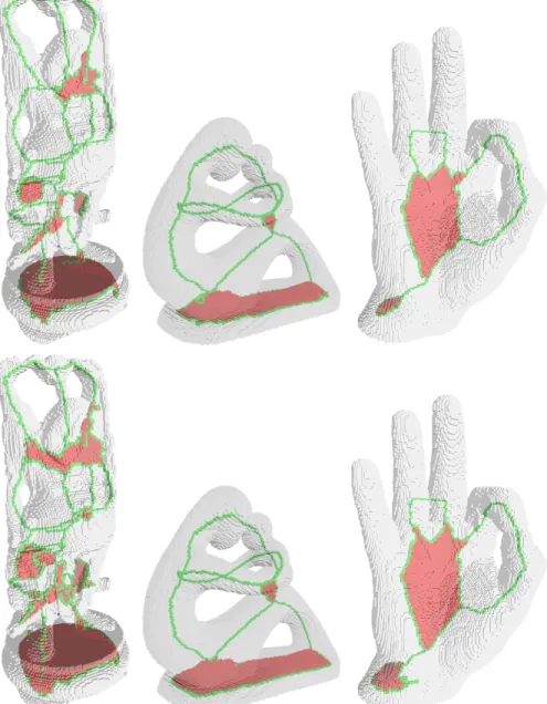
Seeing points or edges belonging to big cellular skeletons can be difficult. Hence, we propose a voxelized version of the cellular skeleton. Its construction is quite simple: every cubical cell [a1, a2] × [b1, b2] × [c1, c2] produces all the possible

voxels (a1, b1, c1), (a2, b1, c1), (a1, b2, c1), (a2, b2, c1), (a1, b1, c2), . . .. These voxels

are coloured following the dimension of the cubical cell which created them: red for 2-cubes, green for 1-cubes and blue for 0-cubes.

Figure 4 compares some cellular skeletons obtained with our algorithm and [LCLJ10] over some voxels sets. Let us remark that both give similar results, even on the third example, which does not keep all the fingers. There is the need to study further how different fixed orders in the elementary collapses affect both algorithms. Also, we observe that upper skeletons are thinner. Hence, we intend to study whether we can obtain even more similar skeletons by adjusting the thresholds.

5

Conclusion and Future Perspectives

The present paper introduces a new kind of skeleton for binary volumes which is a chain complex together with a reduction, which is obtained by a three-step method. It works for different connectivity relations and it does not make use of look-up tables. Our main contribution is the third step, which is completely

new and provides an alternative skeleton representation, synthesizing further homology computations and geometric representation (each cell in the cellular skeleton actually stands for a piece of manifold in the geometric skeleton).

Our future goals are:

– to better understand the difference between choosing the primal or the dual associated cubical complex. The primal associated cubical complex contains more cells, and this can affect the complexity of our algorithms;

– to study different thresholds for the second step. Since it differs from [LCLJ10], we need to study further appropriate thresholds;

– to estimate the complexity of our method.

Acknowledgement

The hand and the statue datasets are courtesy of Michel Couprie, and the Happy Buddha is courtesy of the Stanford University Computer Graphics Laboratory.

References

[Blu67] Harry Blum. A Transformation for Extracting New Descriptors of Shape.

In Weiant Wathen-Dunn, editor, Models for the Perception of Speech and Visual Form, pages 362–380. MIT Press, Cambridge, 1967.

[CB14] Michel Couprie and Gilles Bertrand. Isthmus-based parallel and

asym-metric 3D thinning algorithms. In Discrete Geometry for Computer Im-agery - 18th IAPR International Conference, DGCI 2014, Siena, Italy, September 10-12, 2014. Proceedings, pages 51–62, 2014.

[CC09] John Chaussard and Michel Couprie. Surface thinning in 3D cubical

complexes. In Petra Wiederhold and Reneta P. Barneva, editors, Com-binatorial Image Analysis, volume 5852 of Lecture Notes in Computer Science, pages 135–148. Springer Berlin Heidelberg, 2009.

[Cou11] Michel Couprie. Hierarchic Euclidean skeletons in cubical complexes.

In Isabelle Debled-Rennesson, Eric Domenjoud, Bertrand Kerautret, and Philippe Even, editors, Discrete Geometry for Computer Imagery, vol-ume 6607 of Lecture Notes in Computer Science, pages 141–152. Springer Berlin Heidelberg, 2011.

[Cou13] Michel Couprie. Topological maps and robust hierarchical Euclidean

skeletons in cubical complexes. Computer Vision and Image Understand-ing, 117(4):355–369, 2013. Special issue on Discrete Geometry for Com-puter Imagery.

[DGt] DGtal: Digital geometry tools and algorithms library. http://dgtal.org.

[DS14] P. Dlotko and R. Specogna. Topology preserving thinning of cell

com-plexes. Image Processing, IEEE Transactions on, 23(10):4486–4495, Oct 2014.

[EL53] Samuel Eilenberg and Saunders Mac Lane. On the groups h(π, n), i.

Annals of Mathematics, 58(1):55–106, 1953.

[For02] Robin Forman. A user’s guide to discrete Morse theory. Seminaire

[GBMR14] Aldo Gonzalez-Lorenzo, Alexandra Bac, Jean-Luc Mari, and Pedro Real. Computing homological information based on directed graphs within dis-crete objects. In 16th International Symposium on Symbolic and Numeric Algorithms for Scientific Computing, SYNASC 2014, Timisoara, Roma-nia, September 22-25, 2014, pages 571–578, 2014.

[GSdA+09] J¨urgen Gall, Carsten Stoll, Edilson de Aguiar, Christian Theobalt, Bodo

Rosenhahn, and Hans-Peter Seidel. Motion capture using joint skeleton tracking and surface estimation. In 2009 IEEE Conference on Computer Vision and Pattern Recognition : CVPR 2009, pages 1746–1753, Miami, USA, 2009. IEEE.

[KMM04] T Kaczynski, K Mischaikow, and M Mrozek. Computational Homology,

volume 157, chapter 2, 7, pages 255–258. Springer, 2004.

[KR89] T.Y Kong and A Rosenfeld. Digital topology: Introduction and survey.

Computer Vision, Graphics, and Image Processing, 48(3):357–393, 1989.

[LB07] Christophe Lohou and Gilles Bertrand. Two symmetrical thinning

algo-rithms for 3D binary images, based on P-simple points. Pattern Recogni-tion, 40(8):2301–2314, 2007.

[LCLJ10] L. Liu, E. W. Chambers, D. Letscher, and T. Ju. A simple and

ro-bust thinning algorithm on cell complexes. Computer Graphics Forum, 29(7):2253–2260, 2010.

[LS87] Larry Lambe and Jim Stasheff. Applications of perturbation theory to

iterated fibrations. Manuscripta Mathematica, 58(3):363–376, 1987.

[Mar09] Jean-Luc Mari. Surface sketching with a voxel-based skeleton. In Sreko

Brlek, Christophe Reutenauer, and Xavier Provenal, editors, Discrete Ge-ometry for Computer Imagery, volume 5810 of Lecture Notes in Computer Science, pages 325–336. Springer Berlin Heidelberg, 2009.

[Ser92] Francis Sergeraert. Effective homology, a survey. http://www-fourier.

ujf-grenoble.fr/~sergerar/Papers/Survey.pdf, 1992. [Online;

ac-cessed 11-June-2014].

[Whi50] J. H. C. Whitehead. Simple homotopy types. American Journal of

Math-ematics, 72(1):1–57, 1950.

[YWZ08] Kai Yu, Jiangqin Wu, and Yueting Zhuang. Skeleton-based

recogni-tion of chinese calligraphic character image. In Yueh-MinRay Huang, Changsheng Xu, Kuo-Sheng Cheng, Jar-FerrKevin Yang, M.N.S. Swamy, Shipeng Li, and Jen-Wen Ding, editors, Advances in Multimedia Informa-tion Processing - PCM 2008, Lecture Notes in Computer Science, pages 228–237. Springer Berlin Heidelberg, 2008.

Fig. 4: Top: cellular skeletons computed using the proposed method. Bottom: cellular skeletons computed with the algorithm in [LCLJ10].