Evolution and Development of the Strepsirrhine Primate Skull

HAL Id: tel-01874272

https://hal.archives-ouvertes.fr/tel-01874272

Submitted on 14 Sep 2018

HAL is a multi-disciplinary open access

archive for the deposit and dissemination of sci-entific research documents, whether they are pub-lished or not. The documents may come from teaching and research institutions in France or abroad, or from public or private research centers.

L’archive ouverte pluridisciplinaire HAL, est destinée au dépôt et à la diffusion de documents scientifiques de niveau recherche, publiés ou non, émanant des établissements d’enseignement et de recherche français ou étrangers, des laboratoires publics ou privés.

Skull

Renaud Lebrun

To cite this version:

Renaud Lebrun. Evolution and Development of the Strepsirrhine Primate Skull. Paleontology. Uni-versité de Montpellier 2; Universität Zürich - Switzerland, 2008. English. �tel-01874272�

Dissertation zur

Erlangung der naturwissenschaftlichen Doktorwürde (Dr. sc. nat.) vorgelegt der Mathematisch-naturwissenschaftlichen Fakultät der Universität Zürich

Doppeldoktorat

Prof. Dr. Jean-Jacques Jaeger (Leitung der Dissertation) Dr. Marcia Ponce de León

Prof. Dr. Christoph Zollikofer (Leitung der Dissertation)

pour obtenir le grade de

DOCTEUR DE L’UNIVERSITE MONTPELLIER II

Discipline : Paléontologie Ecole Doctorale : S.I.B.A.G.H.E

-Thèse de doctorat double entre l’UNIVERSITE MONTPELLIER II

et

l’UNIVERSITE de ZÜRICH

présentée et soutenue publiquement par

Renaud Lebrun

Le 04 avril 2008

Titre :

EVOLUTION AND DEVELOPMENT OF THE STREPSIRRHINE PRIMATE SKULL

Rapporteurs

Prof. Dr. William Hylander, . . . .Rapporteur Dr. Christopher Beard, . . . .Rapporteur

Jury

Prof. Dr. Monique Vianey-Liaud, . . . .Présidente du Jury Dr. Franck Guy, . . . .Examinateur Prof. Dr. Jean-Jacques Jaeger, . . . Directeur de Thèse Prof. Dr. William Hylander, . . . Membre invité Dr. Marcia Ponce de León, . . . .Examinateur Prof. Dr. Marcelo Sánchez, . . . .Examinateur Prof. Dr. Christoph Zollikofer, . . . Directeur de Thèse

Since Haeckel (1866), the evolutionary modification of ontogeny has been recognized as an important source of morphological innovation. Due to recent advances in developmental ge-netics and phenotypic analysis, evolutionary developmental (evo-devo) studies have regained considerable interest and led to fundamental changes in our understanding of how ontogeny and phylogeny are related.

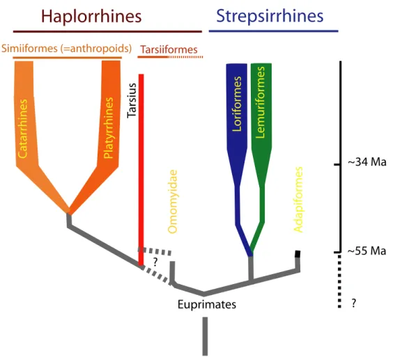
This thesis investigates the relationship between ontogeny and phylogeny in strepsirrhine primates. The suborder Strepsirrhini, which comprises galagos, lorises and Malagasy lemurs, is thought to have retained most of the ancestral primate condition (as opposed to the suborder Haplorrhini, which comprises tarsiers and anthropoids). Nevertheless, strepsirrhines are highly diverse in their morphology. Here, the focus is on cranial diversity, which is analyzed from a developmental perspective with a new set of geometric morphometric tools.

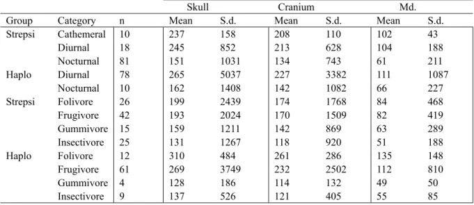
First, patterns of cranio-mandibular variability in extant adult primates are analyzed. Taking into account the phylogenetic constraints applying to the skull morphology permits a quantifi-cation of how dietary specialization and activity patterns influence cranio-mandibular morphol-ogy in both primates suborders. Also, the skull morpholmorphol-ogy in strepsirrhines and haplorrhines is clearly distinct, and it is shown here that differences between and within infraorders can be traced back to differences in developmental modes.

According to a hypothesis proposed by Beard (1988), “strepsirrhinism” represents the prim-itive condition of the primate skull. This thesis shows that the cranial morphology of the Omo-myidae – a basal haplorrhine taxon comprising the genera Rooneyia, Necrolemur and Micro-choerus – is closer to that of extant strepsirrhines than to that of haplorrhines, while the cranial morphology of Tarsius is closer to that of other extant haplorrhines, i.e., the anthropoids. Thus, it is probable that the shift towards a modern haplorrhine morphology occurred in one omomyid lineage, to the exclusion of the three genera mentioned above.

New arguments are proposed to support the hypothesis that the cranio-mandibular mor-phologies of the cheirogaleids and galagids are the least derived from the ancestral condition of toothcombed strepsirrhines.

This thesis presents a comparative geometric morphometric analysis of cranio-mandibular development in ten strepsirrhine and two haplorrhine species. Haplorrhines and strepsirrhines differ widely in ontogenetic trajectory direction, length and position. Within the strepsirrhines, divergence between taxon-specific ontogenetic trajectories and allometric grade shifts are more pronounced in lemurs than in lorises. This pattern of evolutionary modification of ontogenetic trajectories is interpreted in the context of the rapid adaptive radiation of lemurs.

The last section uses insights obtained from the evolutionary developmental analysis of extant taxa for a comparative analysis of fossil strepsirrhine taxa. The morphologies of extant and extinct strepsirrhines are compared. In particular, the morphology of the skull is well known from two adapiform subfamilies, Adapinae and Notharctinae. Among the adapines, a size increase has

oc-in this genus. Adapiforms exhibit longer ontogenetic trajectories than extant strepsirrhoc-ines. A trend toward a shortening of ontogenetic trajectories has occurred in the evolutionary history of strep-sirrhines. This can be related to a context of general increase in encephalization within this lineage.

Abstract . . . . 1

Introduction . . . . 1

Chapter 1 . Materials and Methods . . . . 9

1 . Materials . . . .11

1.1 Taxonomic framework . . . 11

1.2 Sample . . . 11

1.3 CT data acquisition . . . 12

1.4 Reconstruction . . . 12

2 . Methods used throughout this manuscript . . . .13

2.1 Landmark protocols and landmark acquisition . . . 16

2.2 Procrustes superimposition . . . 17

2.3 Principal Component Analysis (PCA) . . . 18

2.4 Canonical Variate Analysis (CVA) and classification procedures. . . 18

2.5 Allometry . . . 19

2.6 Visualization of the results. . . 22

3 . MorphoTools: a geometric morphometric application framework . . . .24

3.1 General architecture of MorphoTools. . . 25

3.2 The sample scheme . . . 26

3.3 Visualization and outputs . . . 30

Chapter 2 . What determines the morphological variation of the primate

skull? . . . . 33

1 . Introduction . . . .35

2 . Materials and methods . . . .38

2.1 Sample composition . . . 38

2.2 Dietary and activity patterns categories used for the study of adaptation . . . 38

2.3 Methods . . . 39

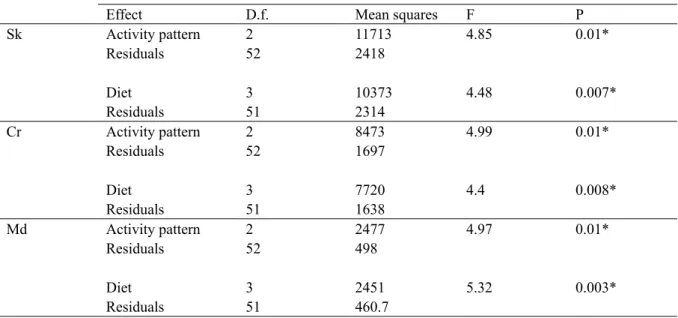
3 . Results . . . .44

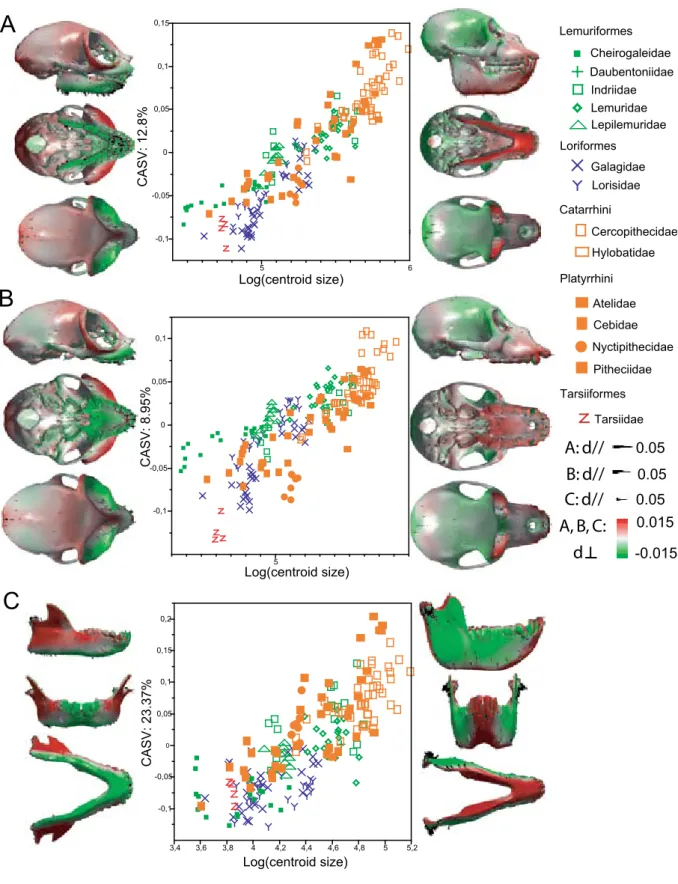
3.1 Patterns of shape variability . . . 44

3.2 The effects of adaptation on the skull morphology . . . 46

3.3 Phylogenetic constraints in primate skulls . . . 53

4 . Discussion . . . .54

4.1 Morphology and adaptation. . . 54

4.2 Phylogenetic constraints explain the morphological differences between haplorrhines and strepsirrhines . . . 56

Chapter 3 . “Strepsirrhinism”: is it a primitive or derived condition in

pri-mates? . . . . 61

1 . Introduction . . . .63

2 . Materials and Methods . . . .64

3 . Results . . . .65

3.1 PCA and classification procedure . . . 65

3.2 Phenetic analysis . . . 67

4 . Discussion . . . .67

4.1 Rooneyia and the validity of A Protoanthropoidea taxon . . . 67

4.2 The ancestral condition of the primate skull architecture . . . 68

Chapter 4 . Patterns of morphological variability in the strepsirrhine skull . 73

2 . Materials and Methods . . . .76

2.1 Sample composition . . . 76

2.2 Methods . . . 76

3 . Results . . . .80

3.1 General patterns of shape variability . . . 80

3.2 Family-specific allometric patterns . . . 84

3.3 Morphology is distinctive at the family level . . . 87

3.4 Estimation of the ancestral morphology of toothcombed strepsirrhines. . . 90

4 . Discussion . . . .90

4.1 Allometry . . . 90

4.2 The ancestral morphology of toothcombed strepsirrhines . . . 92

1 . Introduction . . . .97

2 . Materials and methods . . . .99

2.1 Sample composition . . . 99

2.2 Landmark protocol . . . 99

2.3 Common time scales. . . 99

2.4 The allometric component of ontogenetic shape change . . . 100

2.5 Patterns of shape change during ontogeny . . . 100

2.6 Interspecific differences in ontogenetic trajectory direction, length and position . 101 2.7 Differences between lemuriform and loriform species in ontogenetic trajectory di-vergence. . . 103

2.8 The prenatal and postnatal components of shape change . . . 104

3 . Results . . . .104

3.1 The allometric component of ontogenetic shape change . . . 104

3.2 Postnatal developmental patterns . . . 106

3.3 Interspecific differences in allometric grade . . . 108

3.4 Diversity in ontogenetic trajectories and morphological diversity . . . 111

3.5 Patterns of eruption of the tooth-comb across strepsirrhines species. . . . 113

4 . Discussion . . . .117

4.1 Differences in developmental constraints between haplorrhines and strepsirrhines . . 117 4.2 Trends in the evolution of morphology of the skull in strepsirrhines . . . 117

1 . Introduction . . . .125

2 . Materials and methods . . . .127

2.1 Sample composition . . . 127

2.2 Methods of analysis . . . 127

3 . Results . . . .130

3.1 Shape and size variance in the adapine cranium . . . 130

3.2 Classification procedures . . . 131

3.3 Differences in morphology between adapiforms and toothcombed strepsirrhines 132 3.4 Ontogenetic allometric patterns . . . 136

4 . Discussion . . . .138

4.1 Adapiformes and the cranio-mandibular morphology of stem toothcombed strepsir-rhines. . . 138

4.2 The morphology of the adapine skull . . . 139

4.3 Allometric grade shifts and phyletic gigantism in Leptadapis . . . . 140

4.4 Encephalization and the evolution of development in Strepsirrhines . . . 141

Conclusion . . . . 145

References . . . . 151

Résumé . . . . 173

Acknowledgements . . . . 185

Appendices . . . . 187

Chapter 6: the Adapiformes and the evolution of

the strepsirrhine skull

Introduction

Since Darwin (1859) and Haeckel (1866), it has been recognized that developmental and evolutionary processes model morphology on different time scales: in the long term, morphol-ogy reflects evolution by means of natural selection and adaptation to the environment. On a shorter time scale, morphology is the result of ontogeny and is governed by genetic programs and developmental constraints. The basic thrust behind evolutionary developmental biology, or “evo-devo”, is the proposition that the modification of ontogeny is a major source of morpho-logical innovation during evolution. Within a group of species, morphomorpho-logical diversity can be understood in terms of diversity of species-specific developmental trajectories, which results from modification of the ancestral ontogenetic programs. Today, evo-devo is a growing re-search area, the general aim of which is to establish new ties between development (ontogeny) and evolution (phylogeny) (see Carroll, 2005).

Haeckel’s theory of recapitulation inspired research in evolutionary developmental biol-ogy for almost a century: its principal postulates are that extant species recapitulate the adult stages of their ancestors during ontogeny, and that evolution of new morphologies proceeds by terminal addition of new features. Haeckels notorious proposition that “ontogeny recapitulates phylogeny” inspired a profusion of theoretical and empirical investigations into the connections between ontogeny and phylogeny.

Notably, Haeckel (1866), in an attempt to account for the exceptions to recapitulation, intro-duced the concept of heterochrony as the temporal agent of evolutionary change during ontoge-ny. Heterochrony was redefined by de Beer (1930) as “shifts in timing of an organ relative to the same organ of an ancestor”. De Beer’s redefinition of heterochrony still prevails and currently forms one of the dominant concepts of evolutionary developmental biology. While Haeckel’s original hypothesis of recapitulation was progressively falsified during the 20th_{century, and} while 20th_{-century evolutionary biology had a strong focus on adaptive changes related to} natu-ral selection, Gould’s seminal book “Ontogeny and Phylogeny” (1977) has stimulated regained interest in developmental studies, setting the framework of heterochrony at a central place in the evo-devo field. Heterochrony sensu Gould applies to comparative analysis of shape-age trajec-tories (e.g., Gould, 1977, 2000). The terminology has subsequently been expanded to encom-pass the comparative description of size-age trajectories (Godfrey and Sutherland, 1995; Klin-genberg, 1998; Rice, 1997). Originally restricted to the description of morphological patterns, recent advances in molecular developmental genetics have widened the scope of heterochronic analysis to the genetic processes responsible for observed differences in developmental patterns (e.g., see Ambros, 1997; Fondon and Garner, 2004; Moss, 2007; Slack and Ruvkun, 1997).

In parallel with progress in molecular genetics, the advent of geometric morphometric methods marked a milestone in quantitative phenotypic analysis (e.g., see Bookstein, 1991; Dryden and Mardia, 1998; Marcus et al., 1996). Geometric morphometric methods permit to quantify phenotypic changes that occur during ontogeny and phylogeny in a statistically sound and visually comprehensive manner, permitting the analysis of complex patterns of shape

vari-ability at an unprecedented level of detail.These techniques havetriggered new interest in the description and analysis of patterns of growth and development from an evo-devo perspective, especially in the field of physical anthropology (e.g. see O’Higgins et al., 2001; O’Higgins and Jones, 1998; Ponce de León and Zollikofer, 2001).

A central topic in the field of evo-devo is the hypothesis of human neoteny, which was ini-tially proposed by Bolk (1926) and contemporaries (see Schultz, 1927). Adult humans present characters, especially in the skull, that correspond to the juvenile condition in great apes. Sub-sequent to the major review by Gould (1977) in favor of this hypothesis, the question of human neoteny received considerable attention and yielded controversial debates that lack consensus even today (e.g., see Godfrey and Sutherland, 1996; Penin et al., 2002; Raff, 1996; Rice, 1997; Shea, 1989). In primates, another prime example is the case of Pan paniscus, the pygmy chim-panzee, which has been regarded as a paedomorphic relative of Pan troglodytes since its dis-covery (see. Coolidge, 1933; Schwarz, 1929). Since then, many studies have attempted to test this hypothesis for cranial ontogeny using either a traditional morphometric approach based on linear measurements (e.g., see Shea, 1983a, 1983b, 1989) or geometric morphometric methods (Lieberman et al., 2007; Mitteroecker et al., 2005; Ponce de León and Zollikofer, 2006). Apart from hominoid primates, geometric morphometrics has also been used to analyze the ontogeny of the skull in long-faced old-world monkey species (mandrills, geladas and baboons) in order to assess whether the similarities in morphological patterns observed in adults are produced via homologous morphogenetic processes (e.g., see Collard and O’Higgins, 2001; Leigh, 2006, 2007).

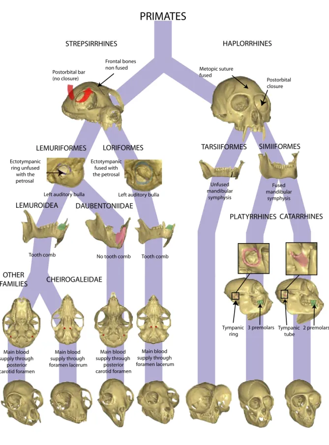
Evo-devo studies addressing questions of anthropoid primate diversity assume a special place because they concern our own evolutionary history. Nevertheless, it is surprising that the enormous diversity of strepsirrhine primates has little been studied from an evo-devo per-spective. This is where the present thesis is situated; it represents an attempt to establish links between ontogenetic and phylogenetic diversity within strepsirrhine primates. Given that di-versity concerns almost every aspect of strepsirrhine biology, the prospects for such an ap-proach are promising: the suborder Strepsirrhini consists of two monophyletic infraorders, the Lemuriformes (the Malagasy lemurs) and the Loriformes, which contains lorises and galagos (as opposed to the suborder Haplorrhini, which contains anthropoids and tarsiers, see Figure 1). Lemuriforms have evolved in isolation on Madagascar during most of the Cenozoic era and occupy a wide range of ecological niches (Mittermeier et al., 1994). Malagasy primates exhibit a wide variety of dietary habits (frugivory, insectivory, folivory, gummivory) and activity pat-terns (diurnality, cathemerality, nocturnality). They also exhibit a wide range of locomotor and postural adaptations (arboreal and terrestrial quadrupedalism, vertical clinging and leaping, and suspension), and body mass ranges between 55 g in Microcebus to about 200 kg in Archaeoin-dri. Thus, the model of adaptive radiation (Simpson, 1953) applies well to the evolutionary history of lemuriform primates: their biological diversification is associated with a broad

eco-logical and phenotypic diversity (Martin, 1972). Conversely, loriform species occupy more restricted ecological niches; competition with haplorrhines probably restricted their diversifica-tion (Mittermeier et al., 1994). Also, there are still open quesdiversifica-tions regarding the evoludiversifica-tionary history of strepsirrhines, the major one being that there is currently no clear fossil evidence for the ancestors of extant strepsirrhines. A group of early strepsirrhines is well-represented in the fossil record: the Eocene adapiforms. Their evolution is well-documented in the Eocene depos-its of Europe, America and Asia. The best-known morphological diversification episode in their evolutionary history is the radiation of the Adapinae subfamily, which occurred from the middle to the late Eocene in Europe (Franzen, 2003; Godinot, 1998; Lanèque, 1992a, 1992b, 1993). Adapiforms did not evolve a toothcomb (composed of elongated, slender and procumbent inci-sors and canines on the jaws), which characterizes extant strepsirrhines. Despite the lack of that character in adapiform primates, even in an incipient state, many researchers have attempted to identify a possible ancestor of toothcombed strepsirrhines among the adapiforms (e.g., see Beard et al., 1988; Beard and Godinot, 1988; Godinot, 1998; 2006 ; Rasmussen and Nekaris, 1998; Seiffert, 2005; Seiffert et al., 2003), but the result of these studies still lack consensus. Fortunately, the fossil record comprises complete skulls of several adapiform taxa, the morphol-ogy of which can be compared to that of modern forms.

Euprimates Lemur ifor mes Omom yidae C atar rhines Pla tyr rhines ? ~34 Ma ~55 Ma

Haplorrhines

Strepsirrhines

Studies focusing on the development of the skull in strepsirrhine primates are typically based on linear measurements (e.g. see Ravosa, 1992, 2007), and their principal aim is to es-tablish links between patterns of growth and development on the one hand, and life-history parameters and strategies on the other (see Godfrey et al., 2004; Godfrey et al., 2005; Smith, 2000). However, these studies do not provide detailed information on changes in shape and size during the ontogeny of the cranium and mandible. Furthermore, they do not compare data belonging to extant and extinct species. As a result, these studies do not indicate how the evolu-tionary modification of ontogenetic trajectories is related to morphological diversification and adaptation. Overall, therefore, little is known about possible links between ontogeny patterns of the skull and phylogenetic diversification in strepsirrhine primates. One major reason for the relatively small number of ontogenetic analyses of cranial morphology (e.g., see Godfrey et al., 2004; Godfrey et al., 2005; King et al., 2001; Ravosa, 1992, 2007; Ravosa and Simons, 1994) is that most collections of juvenile strepsirrhine specimens consist of unprepared cadavers, the osseous structures of which are difficult to access. Thanks to recent developments in 3D micro-tomography (e.g., see Rossi et al., 2003; Silcox, 2003; Spoor, 1998; Tafforeau et al., 2006), it is now possible to perform scans with sufficient spatial resolution to access the skeletal morphol-ogy even in juvenile specimens of the smallest strepsirrhine species, such as Microcebus muri-nus. Furthermore, the use of computer-assisted techniques on CT data offers the opportunity to analyze the morphology of fossils from a whole new perspective: reconstructions of incomplete and distorted specimens can be achieved, which permits to conduct comparative analyses of fossil and extinct forms (Zollikofer and Ponce de León, 1995; Zollikofer et al., 1995).

The main aim of this thesis is to investigate how evolutionary modification of develop-mental programs have contributed to the morphological diversity observed in fossil and extant strepsirrhines. In this thesis, the focus is on skull morphology because:

the skull conveys a strong phylogenetic signal, which is traditionally used for systematic -

analyses (for instance, see Cartmill, 1994; Fleagle, 1999; Kay et al., 1997; MacPhee and Cartmill, 1986; Shoshani et al., 1996);

the skull houses the masticatory apparatus, the brain and the major sense organs; skull -

morphology is expected to reflect various functional adaptations that are of interest for evolutionary studies;

the skull is a 3D biological structure with many quantifiable features of interest, and -

homologous locations; thus, it is possible to conduct comparative analyses using 3D geometric morphometric methods.

The following specific issues are addressed: Methods

1) : How can complex and diverse patterns of craniomandibular morphological variation (in phyletic and ontogenetic time) be analyzed comprehensively? What would be the benefits of using an integrated geometric morphometric application framework in order to conduct such analyses?

Functional versus developmental constraints

2) : What is the relative contribution of

functional adaptation and developmental constraints on primate skull size and shape? This issue concerns the debate between adaptationists and structuralists (Gould and Lewontin, 1979).

Ontogenetic sources of phyletic diversity

3) : What are the relationships between

developmental diversity and species diversity? Evo-devo perspective on fossil taxa

4) : What is the link between the increase in

encephalization in strepsirrhine primates and the evolution of the development of the skull?

These issues are investigated in this manuscript throughout six chapters. Chapter 1 is dedi-cated to the methods and analytic tools used throughout the thesis. An integrated geometric morphometric software is presented that permits interactive and comprehensive analysis and visualization of patterns of shape variability in 3D biological structures, such as the skull.

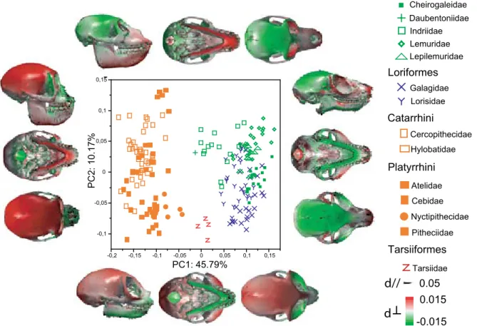
In Chapter 2, a sample of adult strepsirrhine and haplorrhine skulls is studied: we examined whether the two suborders share similar patterns of shape variation. Then, taking into account the phylogenetic signal conveyed by the morphology in both infraorders, the extent to which dietary specialization and activity patterns impinge on the morphology of the skull in haplor-rhines and strepsirhaplor-rhines is assessed.

According to a hypothesis proposed by Beard (1988), “anatomical strepsirrhinism” repre-sents the primitive condition in primates. In order to test whether this hypothesis also applies to the global morphology of the cranium, Chapter 3 presents a geometric morphometric analysis of a sample composed of crania of basal haplorrhine fossils belonging to the Omomyidae fam-ily and extant haplorrhine and strepsirrhine crania.

Chapter 4 provides an analysis of the morphological variability of the skull of extant adult strepsirrhines. Among strepsirrhines, a popular hypothesis proposes that cheirogaleids and galagids have retained the most of the ancestral toothcombed strepsirrhine condition. This hy-pothesis is examined for the morphology of the skull using both geometric morphometric and phylogenetically based comparative approaches.

In Chapter 5, a comparative analysis of the developmental patterns of a sample composed of ten strepsirrhine and two haplorrhine species is conducted. The following issues are investigat-ed. What are the differences and commonalities between strepsirrhine and haplorrhine patterns of ontogeny? Is it possible to link the diversity of developmental patterns in lemuriforms with their adaptive radiation? Does this diversity stand in marked contrast with the developmental patterns observed in less diversified groups such as the Loriformes?

In Chapter 6, the morphologies of extant and extinct strepsirrhines are compared. Cranio-mandibular morphology is well-known in two subfamilies of Adapiformes, the Adapinae and the Notharctinae. Patterns of morphological diversity of the adapiform skull are compared with those of extant strepsirrhines using insights obtained from the developmental analysis of extant

Chapter 6: the Adapiformes and the evolution of

the strepsirrhine skull

Materials and Methods

Chapter 1

Chapter 1. Materials and Methods

Contents

2 . Methods used throughout this manuscript . . . .13

2.1 Landmark protocols and landmark acquisition . . . 16

2.2 Procrustes superimposition . . . 17

2.3 Principal Component Analysis (PCA) . . . 18

2.4 Canonical Variate Analysis (CVA) and classification procedures. . . 18

2.5 Allometry . . . 19

2.6 Visualization of the results. . . 22

3 . MorphoTools: a geometric morphometric application framework . . . .24

3.1 General architecture of MorphoTools. . . 25

3.2 The sample scheme . . . 26

Materials 1.

Taxonomic framework 1.1

In this manuscript, the systematic taxonomy proposed by Groves (2001) was followed, with the following exceptions. Strong molecular evidence suggests that the Malagasy lemurs are monophyletic and that the genus Daubentonia is basal in this group (e.g., see Roos et al., 2004; Yoder and Yang, 2004). Therefore, the infraroder “Lemuriformes” was used to designate all Malagasy primates (no use was made of the infraorder “Chiromyiformes”, within which Groves (2001) places Daubentonia). Thus, it was considered that the suborder Strepsirrhini comprises only two extant infraorders: Loriformes and Lemuriformes. Following Gunnell and Rose (2002), the term Tarsiiformes here designates Tarsius and the Omomyidae family.

Sample 1.2

Morphological data were collected from 311 distinct specimens that consisted of 285 com-plete skulls, 22 isolated crania or crania associated with badly preserved mandibles and 4 iso-lated mandibles. This sample comprises adults of extant species, juveniles of extant species and adults of extinct species.

Adults belonging to extant and recently extinct species 1.2.1

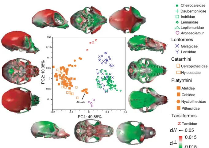
Morphological data were collected from 205 extant adult primate individuals, 115 of which are strepsirrhines and 90 are haplorrhines, and all of which have crania with associated man-dibles. The sample also comprises 4 isolated crania and 3 isolated mandibles belonging to 7 in-dividuals of the genus Archaeolemur, a recently extinct lemur of Madagascar. These specimens are listed in Appendix 1.

Extant juveniles 1.2.2

Postnatal ontogenetic data were collected for 10 strepsirrhine species (Lemur catta, Lepil-emur ruficaudatus, Microcebus murinus, Propithecus diadema and Propithecus verreauxi, Arc-tocebus calabarensis, Nycticebus coucang, Perodicticus potto, Galago senegalensis, Otolemur garnetti) and 2 haplorrhine species (Tarsius bancanus and Aotus trivirgatus). The sample com-prises 83 skulls (crania + mandibles) and one isolated cranium belonging to juvenile individu-als. Two mandibles belonging to individuals of the genus Propithecus were badly preserved and, therefore, could not be included in the analyses. As a whole, 81 crania with associated mandibles were analyzed. A comprehensive list of the juvenile specimens is presented in Ap-pendix 1. Additionally, information on the state of dental eruption for each specimen is pro-vided in the Appendices 3.1-12.

Extinct specimens 1.2.3

The fossil sample consists of 11 Eocene adapiform specimens. The sub-family Adapinae is represented by three isolated crania of Adapis sp., four isolated crania and one complete skull of Leptadapis, and the cranium of the type specimen of Palaeolemur betillei, the subfamily Notharctinae by one complete skull of Notharctus tenebrosus and one cranium of Smilodectes gracilis. Additionally, four crania belonging to the Eocene Omomyidae family are included in the sample. The sub-family Microchoerinae is represented by Necrolemur (N=2) and Micro-choerus (N=1), and the tribe Rooneyinii is represented by the cranium of the type specimen of Rooneyia viejaensis. The cast of the cranium of Rooneyia was scanned using a 3D laser scanner by Sai Man Wong, the assistant of Pr. A. Rosenberger, for the purposes of a recently published work (Rosenberger, 2006). The complete Eocene fossil list is presented in Appendix 2.

CT data acquisition 1.3

205 specimens were scanned using tomography (N=8), conventional microtomography (N=166) and microtomography using synchrotron light (N=31). Microtomography yields high-resolution cross-sectional image series of cranial and mandibular structures (see specimen lists presented in Appendix 1 and Appendix 2). Four fossils were scanned at the European Synchro-tron Radiation Facility (E.S.R.F) on beamlines ID19 and ID17. The use of synchroSynchro-tron light for mineralized fossils is recommended because it produces far better results than those achieved with conventional industrial scanners (Tafforeau et al., 2006). For a few fossils, only casts were available. Therefore, these samples were CT scanned to produce a 3D representation of the external fossil surface. Each voxel of the CT images stack consists of a measurement of the density of the object of interest at a given location (x,y,z) in space. For all scanned specimens, 3D surface representations were generated from the µCT volume data using the “isosurface” algorithm of the Amira software package (TGS, San Diego, CA). The position of the interface between air and bone is set using the half-maximum height technique (Baxter and Sorenson, 1981; Spoor et al., 1993). The resulting virtual representations of the mandibles and crania were positioned in dental occlusion.

Reconstruction 1.4

Reconstruction of one neonate Propithecus diadema 1.4.1

The cranium of a specimen belonging to the species Propithecus diadema presented several bones that were displaced (see Appendix 4-A). A virtual reconstruction of this specimen was performed in order to recover its original morphology. Groups of bones and individual bones that were displaced were segmented and repositioned in their original anatomical locations. Ad-ditionally, bones missing from the left orbital region were reconstructed using mirror images of

the corresponding bones (see Appendix 4 for details). Fossils

1.4.2

Several fossils and extant specimens were incomplete, were deformed or presented dis-placed parts. Theses specimens were reconstructed following the recommendations of Zollikof-er and Ponce de León (2005). WhenevZollikof-er possible, missing parts wZollikof-ere retrieved using symmetry. Pieces that had been displaced but not deformed were moved to their original position. To guar-antee accurate virtual reconstructions, only relatively undistorted and almost complete fossils were incorporated in the sample. In seven fossils, several missing parts, mostly situated in the orbital region, were reconstructed by producing a mirror image of the corresponding part (see Appendices 5, 6, 7, 8, 9, 10 and 11).

Recommendations given by Zollikofer and Ponce de León (2005) were followed to correct for plastic deformation of the skull of Notharctus tenebrosus that was incorporated in this study. In this case, plastic deformation was principally due to compression. The directions of maximal compression were estimated in the coronal and axial planes, and decompression was subse-quently applied to retrieve the bilateral symmetry of the skull (see Appendix 12). The result-ing virtual representation of the fossil was almost undistorted, but larger than the original one. Thus, this representation was scaled by a factor of 0.95 in order to recover the original size.

Methods used throughout this manuscript 2.

Compared to traditional morphometric methods, which are based on linear and angular measurements, geometric morphometric (GM) methods have two major advantages:

- the biological form is reduced to its size and shape components. In a traditional approach based on linear measurements, this is not possible because the measurements are measure-ments of size, and size is thus expected to be the main source of morphological variation. In a GM context, variation in size does not mask variation in shape, even when the size range of the sample is wide;

- the information conveyed by the geometric structure of the biological object is preserved throughout analysis: it is possible to have a visual representation of the results, which can be interpreted biologically. For a given biological structure, spatial morphological variability pat-terns can be readily identified and visualized comprehensively.

The use of landmarks is common in studies that analyze primate skull morphology (see for instance Mitteroecker et al., 2004a; O’Higgins and Jones, 1998; Ponce de León and Zol-likofer, 2001). When analyzing bones, such as the skull, landmarks can be defined at different loci, such as the intersection of bone sutures, the center of foramina and the tips and maxima of curvature. The basic thrust of GM analyses involving landmarks is the hypothesis of biologi-cal homology of the landmark locations across all specimens of a sample. Bookstein (1991)

proposed a nomenclature that accounts for the quality of the landmarks in terms of homology. Accordingly, type I landmarks are expected to convey more homology information than type II or III landmarks.

All GM analyses performed in this thesis are based on 3D cranial and mandibular land-marks. This methodology provides an efficient means to capture the geometry of the skull in a comprehensive way.

An overview of the different steps of a GM analysis is given in Figure 1.1

1) Definition of a landmark protocol and of the sample

3) Procrustes Alignment 4) Computation of mean specimens (optional) 5) Analysis of procrustes residuals (PCA, CVA, ...) 2) Landmark acquisition for all the specimens 6) Visualization of the results 7) Interpretation of the results

Figure 1.1: Steps of a geometric morphometrics analysis involving landmarks.

1 2 3 6 4 8 8 9 10 12 13 12 14 15 15 16 17 18 11 ₁₀

Table 1.1: Mandibular landmarks used throughout the manuscript. * No analysis of the mandible is conducted in the 3rd _{Chapter. ** Not used for the specific sub-analysis using a comparative sample}

composed of ontogenetic series.

# Name Definition Used in Chapters

2 3* 4 5 6 1 Infradentale midpoint between I1L/I1R on alveolar rim X X X X

2,3 Foramen _mandibulare X X X X

4,5 M3 medial point on buccal crown surface of permanent M3 X X X** 6,7 Ramus point on the anterior rim of the ramus, where it starts sloping _{upward from the alveolar plane, in lateral view} X X X X

8,9 Kondylion highest medial point of the condyle X X X X

10,11 Incisura lowest point of mandibular notch X X X X

12,13 Coronoid _process highest point X X X X

14 Akanthion between spinae mentales X X X X

15 Gnathion inferiormost point on symphysis X X X X

16,17 Gonion location of largest curvature on the gonial edge X X X X

1 2 3 4 5 6 8 10 12 13 14 16 18 20 22 24 26 26 27 24 25 20 21 28 28 29 10 11 30 32 32 14 15 33 34 34 35 36 38 38 39 40 39 41 42 43 44 44 45 45 46 47 47 48 49 49 50 51 52 53 54

Table 1.2: Cranial landmarks used throughout the manuscript. * Not used for the specific sub-analysis using a comparative sample composed of ontogenetic series.

# Name Definition Used in Chapters

2 3 4 5 6

1 Nasion X X X

2 Mid nasion-bregma Midpoint of nasion-bregma arch X X X X X

3 Bregma X X X X X

4 Mid bregma-lambda X X X

5 Lambda

6,7 Mid coronale Midpoint of coronal suture between pterion (fronto-_{sphenoid suture) and bregma} X X X X X 8,9 Mid lambda Midpoint of lambda suture between asterion and _lambda X X X X X 10,11 Pterion Meeting poit of coronal with sphenoid suture X X X X X

12 Nasospinale X X X

13 Rhinion X X X

14,15 Apertura nasalis Lateralmost points on the nasal aperture X X X 16,17 Maxillofrontale Anterior edge of maxillofrontal suture X X X X X

18,19 Highest orbital point X X X X X

20,21 Orbitale (or) Zygomatico-maxillary suture X X X X X

22,23 Frontomalare-_{Orbitale (fmo)} Fronto-zygomatic suture at the orbital rim X X X X 24,25 Mid fmo-or Midpoint between fmo and or at the orbital rim X X X X 26,27 Zygomaxillare Zygomatico-maxillary suture at the tuberosity X X X X X 28,29 Jugale Location of largest curvature of the zygomatic rim in _{the jugal region} X X X X X 30, 31 Foramen maxillare Midpoint at the level of the surface X X X X X 32,33 Caninus buccal Buccal midpoint of crown of canine X X X X X 34,35 Third molar (M3) Buccal midpoint of the crown of the last permanent _molar X X X X*

36,37 Asterion X X X X X

38 Mid lambda-_opisthion Midpoint on lambda-opisthion arch X X X 39 Opisthion Posteriormost midpoint of foramen magnum X X X X X 40 Basion Anteriormost midpoint of foramen magnum X X X X X

41 Sphenobasion Midpoint of sphenobasilar suture X X X X X

42 Staphilion Posteriormost midpoint of palate X X X X X

43 Palatum maxillare Sagital point at the suture between the palate and _maxillar. X X X X X

44 Prosthion X X X 45,46 Porion X X X X X 47,48 Stylomastoid _foramen X X X X X 49,50 Foramen ovale X X X X X 51,52 Sutura pterigo-mx X X X X X 53,54 Hypogloss canal X X X X X

Landmark protocols and landmark acquisition 2.1

Protocols 2.1.1

56 cranial and 18 mandibular landmarks were defined (see Table 1.1 and Table 1.2). The combination of these 2 sets of landmarks results in 3 configurations: the mandible configura-tion, the cranium configuration and the cranium plus the mandible in occlusion. Throughout this manuscript, the latter configuration is referred to under the term “skull configuration”. The term “cranium configuration” thus refers to the cranium without the mandible.

Landmarks were defined at the intersection of bone sutures, in the center of foramina and on the tips and maxima of curvature. They consist principally of type I and II landmarks, following the nomenclature defined by Bookstein (1991).

Several landmarks were not used in all of the analyses. In the analyses involving ontogenet-ic series (in Chapter 5 but also in an analysis presented in Chapter 6), the protocols used for the cranium and the mandibular configurations differed only slightly: the landmarks corresponding to the permanent last molar have been omitted.

Concerning the analyses involving the crania of the Omomyidae family (Chapter 3), the corresponding protocol takes into account the fact that most of these fossils are incomplete in the orbital region. Furthermore, in many omomyids and adapiforms, it is also difficult to sat-isfactorily estimate the position of the “lambda” landmark because the corresponding region is often badly preserved. Several fossils are also incomplete in the nasal region. Thus, the cor-responding points do not form part of the protocols used for analyses of samples comprising fossils.

Landmark acquisition 2.1.2

Concerning the 205 specimens that were CT scanned and the specimen scanned using a laser scanner (see lists presented in Appendix 1, Appendix 2 and Appendices 3.1-12), 3D land-marks were digitized on 3D virtual representations derived from the scans. Landmark data from the remaining 105 specimens were digitized on the original specimens using a Microscribe 3D device (see again the lists presented in Appendix 1, Appendix 2 and Appendices 3.1-12). In these cases, the cranium and mandible were digitized separately. Subsequently, these two sets of landmarks were positioned to retrieve occlusion by applying rotations to one of two configu-rations: they were manually aligned together using the points taken at the condyles and on the tooth rows as indicators of occlusion.

In neonate specimens exhibiting patent fontanels, the corresponding landmarks were posi-tioned at the location where growing bones are expected to join. All fossils presented canine alveoli, but some of them had lost the corresponding teeth. The corresponding landmark posi-tions were estimated in the following way: they were digitized at the position of the anterior-most point on the canine alveoli at a height corresponding to that of the average height of the

tooth row. Even if this estimation introduced measurement error, these landmarks were kept since they provide a reliable estimate of the total length of the maxilla, an important piece of information that would otherwise be lost.

Concerning the fossils that were measured using the Microscribe 3D device, when one landmark belonging to a couple of symmetric landmarks was missing, a mirror image of the preserved landmark was produced.

Procrustes superimposition 2.2

The landmark configurations measured for the specimens of a given sample are not directly comparable to one another because the system of coordinates in which the specimens are mea-sured and their orientations are not the same. Moreover, the specimens differ in size. Thus, it is necessary to provide a frame of reference within which spatial relationships between landmark configurations can be quantified. One solution was proposed by Lele and Richstmeier (Lele, 1993; Lele and Richtsmeier, 1991; Richtsmeier and Lele, 1993): Euclidean Distance Matrix Analysis (EDMA). This approach consists of including all possible distances within a set of landmarks into a multivariate analysis. However, the results of EDMA are difficult to visualize because it is not possible to re-express variation in distance matrices as morphological variation in physical space.

The alternative approach used here consists of superimposing the landmark configurations using a Generalized Least Squares (GLS) procedure (Rohlf and Slice, 1990) and establishing a multidimensional shape space within which each specimen is represented as a point (Bookstein, 1991; Dryden and Mardia, 1998). This method involves the following steps:

- Size and shape information are separated. Size is estimated by centroid size (CS) (Bookstein, 1991), which is defined as follows:

CS= ;

where c is the center of mass of the landmark configuration, p_i is the i-th landmark, D is the dimensionality (2 or 3) and k is the number of landmarks .

Each landmark configuration is normalized to CS=1. -

All landmark configurations are superimposed using a GLS criterion to minimize -

deviations between configurations. This is achieved by translating and rotating the size-normalized specimens until the sum of all interspecimen distances (landmark coordinate by landmark coordinate) is minimized.

A consensus configuration is computed as the mean of all aligned specimens. The deviation of each specimen (landmark coordinate by landmark coordinate) from the consensus configura-tion defines its shape in linearized Procrustes shape space. These so-called Procrustes residuals





have the same dimensionality as the original landmark configurations (Dk). However, 7 degrees of freedom (DF) are lost during the superimposition process. One DF corresponds to the nor-malization of the configurations to CS=1. Three DF are lost during translation. Finally, 3 DF are lost during rotation. Accordingly, the linearized Procrustes shape space has Dk-7 independent dimensions.

Principal Component Analysis (PCA) 2.3

PCA (Jolliffe, 1986) is a tool that is used to capture statistically significant patterns of varia-tion in a multivariate sample. PCA produces new sets of variables, the principal components (PCs), which are linear combinations of the original variables. The main feature of PCs is that they are statistically independent of each other and capture the largest, second largest, etc., proportions of the total sample variance. Typically, a significant proportion of the total variance is contained in the first few PCs such that it is possible to express the essential patterns of vari-ability in the sample in a low-dimensional subspace of the original multivariate space.

Canonical Variate Analysis (CVA) and classification procedures. 2.4

CVA is a tool that is used to capture the most statistically significant patterns of variation among groups defined a priori in a multivariate sample. In CVA, two variance-covariance ma-trices are examined (see for instance Zelditch et al., 2004). The within-groups variance-covari-ance matrix, S _W, represents the deviation of individuals from their respective group means. The between-groups variance covariance matrix, S_B, represents the deviation of the group means from the grand mean. CVA provides axes in shape space (the so-called Canonical Variate axes, or CVs) that maximize the ratio S_B/S_W. Maximization of this ratio is achieved by computing the eigenvalues and corresponding eigenvectors of S_W-1_S

B (see Zelditch et al., 2004 for further details).

Computation of the inverse of the within-group variance-covariance requires that this ma-trix be of full rank. Thus, Procrustes residuals cannot be used to compute this mama-trix because 7 DF are lost during the superimposition process (see above). Rather, a PCA is first performed on the data in linearized Procrustes shape space. The PC scores of the specimens are then used to compute S_B and S_W.

Scores of the specimens on the canonical axes (canonical scores) are used to classify the specimens. The procedure explained by Zelditch et al. (2004) is employed as follows: for each group, the mean projection in CVA space is computed. Then, the Mahalanobis distance between each specimen and all group means is computed. For a given specimen X and a given group M, this distance is obtained by:

)

(

)

(

X

M

S

X

M

D=

₋

₋

where S-1 _{is the inverse of the variance-covariance matrix of the CV scores of the} speci-mens. The specimens used as the CVA input are then reallocated a posteriori to the group for which D is minimal. The percentage of correct a posteriori reallocations is useful to assess whether distinct shapes are associated with the pre-defined categories. A low percentage of cor-rect reallocations indicates that it is not possible to distinguish the classes by shape. Fossils or specimens for which the classification is uncertain can be projected onto the canonical axes and allocated to a category according to their scores.

Allometry 2.5

Common allometric patterns 2.5.1

Allometry refers to the effects of size upon shape (Gould, 1966). Here, allometric patterns are investigated in data sets that involve multiple primate species and different developmen-tal stages. Ontogenetic allometry stands for a change in shape that occurs during growth, i.e., an increase in size. Intraspecific allometry (also called static allometry) is the effect of size upon shape in a set of adult individuals belonging to the same species. Interspecific allometry (also called evolutionary allometry) is the effect of size upon shape in a set of adult individu-als belonging to related species. Ontogenetic and interspecific allometries can be detected by multivariate regressions of shape against size (Klingenberg, 1996). In the case of geometric morphometric studies involving 3D landmarks, a multivariate regression of Procrustes

residu-Propithecus diadema Microcebus murinus A B -0,1 -0,05 0 0,05 0,1 0,15 C A S V A : 3 5. 5% 4 4,5 5 5,5 Log(centroid size) -0,1 -0,05 0 0,05 0,1 C A S V B : 3 2. 2% 4 4,5 5 5,5 Log(centroid size) -0,1 -0,05 0 0,05 P C 2: 2 6. 57 % -0,1 -0,05 0 0,05 0,1 0,15 PC1: 37.47% C ASV M.m. ASV P.d. CASV B CASV A

Figure 1.2: Quantification of the common effect of allometry in groups that differ in centroid size. A: Com-mon allometric shape vector (CASV) computed directly on a sample composed of ontogenetic series of specimens belonging to the species Microcebus murinus and Propithecus diadema. CASV behaves like a discriminant axis, and separates the two species. B: CASV computed as the mean of the allometric shape vectors (ASVs) computed separately for the two species. This CASV better represents the common patterns of allometry shared by the two species. C: PC1-PC2 plot. The projection on PC1-PC2 scatter of the species-specific ASVs are reported, as well as CASV A and CASV B. ASV M.m.: ASV computed for Microcebus

-0,1 -0,05 0 0,05 S ha pe c om pn en t 2 -0,1 -0,05 0 0,05 0,1 0,15 Shape component 1 -0,1 -0,05 0 0,05 -0,1 -0,05 0 0,05 0,1 0,15 Shape component 1 S ha pe c om pn en t 2 -0,1 -0,05 0 0,05 S ha pe c om pn en t 2 -0,1 -0,05 0 0,05 0,1 0,15 Shape component 1 -0,1 -0,05 0 0,05 -0,1 -0,05 0 0,05 0,1 0,15 Shape component 1 S ha pe c om pn en t 2 ASV1 ASV2

A1: original data A2: resampling of the original data

B1: data corrected for shape B2: resampling of the data corrected for shape

ASV2 ASV1 ASV1 ASV2 ASV1 ASV2

Figure 1.3: Assessment of the statistical significance of the angle of divergence of the allometric vectors in groups that differ in shape. A1: two groups exhibit a significant difference in shape. It is asked whether the angle between ASV1 and ASV2 is significant. A2: individuals are reassigned randomly to one of the two groups. The angle between ASV1 and ASV2 reflects not only divergence in allometric direction, but also difference in shape across the groups. B1: the data are first corrected to achieve a mean shape difference = 0 between the two groups. Here, the angle between ASV1 and ASV2 is the same as in “A1”. B2: the same group resampling is applied as in A2, but on data corrected for shape. The angle between ASV1 and ASV2 only reflects divergence in allometric vector direction.

-0,1 -0,05 0 0,05 S ha pe c om po ne nt 4,4 4,5 4,6 4,7 4,8 4,9 5 5,1 5,2 Log(centroid size) -0,1 -0,05 0 0,05 S ha pe c om po ne nt 4,4 4,5 4,6 4,7 4,8 4,9 5 5,1 5,2 Log(centroid size) -0,1 -0,05 0 0,05 S ha pe c om po ne nt 4,4 4,5 4,6 4,7 4,8 4,9 5 5,1 5,2 Log(centroid size)

A1: original data A2: resampling of the original data

B1: data corrected for size

-0,1 -0,05 0 0,05 S ha pe c om po ne nt 4,4 4,5 4,6 4,7 4,8 4,9 5 5,1 5,2 Log(centroid size) a1 a2 a2 a1

B2: resampling of the data corrected for size

a1

a2

a1

a2

Figure 1.4: Assessment of the statistical significance of the angle of divergence of the allometric vectors in groups that differ in centroid size. A1: two groups exhibit a significant difference in size. It is asked whether their respective allometric shape vectors (ASV1 and ASV2) differ in direction. Each shape component is regressed against the logarithm of centroid size. ASV1 and ASV2 are composed of all regression coefficients (a1 and a2 in this case) of shape coordinates against size. A2: individuals are reassigned randomly to one of the two groups. The regression coefficients a1 and a2 convey a signal that reflects the difference in size across the groups. Therefore, the angle between ASV1 and ASV2 will not reflect divergence in only the allometric direction. B1: the data are corrected to achieve a mean size difference = 0 between the two groups. Here, a1 and a2 are the same as in “A1”. B2: the same group resampling is applied as in A2 but on data corrected for size.

als against centroid size or against the logarithm of centroid size may be performed (see for in-stance Claude et al., 2003; Claude et al., 2004; Ponce de León and Zollikofer, 2006; Zollikofer and Ponce de León, 2004). In practice, choosing centroid size or its logarithm as a proxy for size yields broadly similar results.

Sometimes, samples contain groups that differ widely in size. In such cases, the vector restulting from a direct regression of shape against size often behaves like a discriminant axis; this vector tends to separate groups according to their size. An example is given in Figure 1.2-A: a regression of shape against size is computed in a sample composed of ontogenetic series of specimens belonging to the species Microcebus murinus, one of the smallest extant lemurs, and Propithecus diadema, one of the largest ones. The resulting common allometric shape vec-tor (CASV) discriminates the two species almost perfectly: Microcebus murinus exhibits low scores on the CASV whereas individuals belonging to the species Propithecus diadema exhibit high scores (figure 1.2-A).

In order to produce a CASV that does not behave like a discriminant axis, the approach proposed by Ponce de León and Zollikofer (2006) was used. A CASV is computed as the mean of the group-specific allometric shape vectors (ASVs) (see Figure 1.2-B). The resulting axis describes patterns of allometry that are common to the two species.

Divergence in direction between allometric shape vectors 2.5.2

Resampling statistics are used throughout this manuscript to assess inter-group divergence between allometric vectors. When groups differ widely in shape, a considerable heterogeneity in shape is included in each of the resampled groups (see Figure 1.3), resulting in a biased dis-tribution of angles of divergence. Similarly, a considerable heterogeneity in size (Figure 1.4) is introduced in each of the two resampled groups when the groups under study differ significantly in size. In order to avoid these pitfalls, the test sequence proposed by Ponce de León and Zol-likofer (2006) was adopted with a slight modification to test for inter-group difference in size. 1) Test for differences between mean group values of shape and size.

2) If differences are significant, correct data to achieve mean shape and size difference = 0 between each group (see Figure 1.3-A2 and Figure 1.4-A2).

3) Test for divergence between group specific allometric vectors (using resampling statistics). Visualization of the results.

2.6

As mentioned earlier, one important aspect of geometric morphometric methods is that they allow for visualization of the results. It is possible to visualize morphological variations along the axes of PCAs, CVAs and also the vectors resulting from the regressions of shape against scalars. Throughout this manuscript, the visualization methods proposed by Zollikofer and Ponce de León (2002) were used; they help to explore the patterns of shape variability on

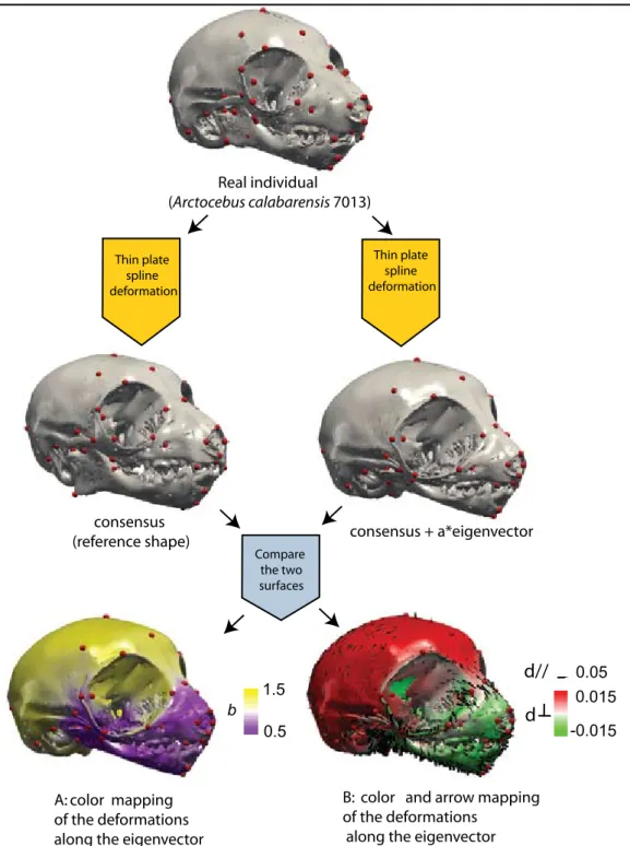
Real individual (Arctocebus calabarensis 7013) consensus + a*eigenvector Compare the two surfaces consensus (reference shape)

B: color and arrow mapping of the deformations

along the eigenvector

Thin plate spline deformation Thin plate spline deformation 0.05 -0.015 0.015 d// d 0.5 1.5 b A: color mapping of the deformations along the eigenvector

Figure 1.5: Patterns of cranio-mandibular shape transformation along an eigenvector. A: colors indicate the relative amount of change in local area that was necessary to attain that shape, with the reference being in that specific example the consensus shape, e.g., the mean shape of a given sample (yellow and violet code for an increase and decrease in surface area, respectively, and white indicates isometry. Scale unit: local area/ same local area of the reference shape). B: colors and arrows indicate the magnitude and direction of the shape change, with the reference shape being the consensus (d//: shape change parallel to the surface. d┴: shape change perpendicular to the surface. Red and green indicate outward and inward directions, respec-tively. Scales are in units of centroid size).

3D surfaces (such as virtual reconstructions extracted from CT images).

In all GM analyses presented in this manuscript, changes in shape that occur along vectors of special interest (PCA eigenvectors, CVA canonical vectors or regression vectors) were quan-tified and mapped onto a given surface using color scales and arrows. In practice, a shape of reference and a shape of interest are needed in order to allow for shape comparison (see Figure 1.5). In all the analyses presented in this thesis, the consensus configuration (e.g., the mean shape of a given sample) was chosen as the reference. In practice, a given individual of the sample is chosen as a template. The corresponding surface is deformed twice using a thin plate spline (TPS) function (Bookstein, 1991) into both the consensus configuration and the configu-ration of interest (e.g., the corresponding configuconfigu-ration of landmarks along an eigenvector). The different landmark configurations constitute the nodes of the TPS function. Two different ways to quantify differences in shape are used in this manuscript. The first quantifies the relative dif-ference in local surface area (Figure 1.5-A) and is adequate to describe patterns of shape change during ontogeny (see Chapter 5). The other quantifies directional shape change (Figure 1.5-B): shape change parallel to the surface is represented by arrows, and shape change perpendicular to the surface is represented by a color scale.

MorphoTools: a geometric morphometric application framework 3.

Typically, a morphometric study aims to measure patterns of morphological variability and test how morphological variability correlates with extrinsic and intrinsic variables. There can be two different kinds of variables: categorical (e.g., a group to which an individual belongs) and continuous (scalars).

The complexity of morphometric analyses increases with the complexity of the sample. What is referred to here under the term “sample complexity” is not sample size but sample structure; when multiple variables are defined, assessing the influence of each individual vari-able and possible combinations of these varivari-ables on morphology is a time-consuming process. Furthermore, the results of the whole analysis also depend on the measurement protocol. It is thus mandatory to test whether the results are robust, i.e., to assess if and how modifications of the measurement protocol influence the results. Another source of potential bias in an analysis is the inclusion of “outliers” (e.g., specimens that deviate considerably from the sample mean). Ordination methods, such as PCA, tend to yield axes that discriminate atypical specimens be-cause they often account for a large part of the total sample variance. Therefore, it is also im-portant to assess how the inclusion of outlier specimens affects the results.

These tests cannot be performed interactively with standard GM software packages. For instance, if one wants to add/remove one specimen or add/remove a landmark, all subsequent steps and associated software manipulations must be redone.

issues (Specht, 2007; Specht et al., 2007; Swiss NFS projects N° 205321-102024/1 and 205320-109303/1). MorphoTools facilitates the interactive analysis and visualization of geo-metric morphogeo-metrics datasets. Here, I give a brief overview of the basic architecture of Mor-phoTools and report on those parts that were implemented within the framework of this thesis.

General architecture of MorphoTools. 3.1

The Visualization Toolkit 3.1.1

The Visualization Toolkit (VTK) (Schroeder et al., 2006) is used at the core of the Mor-phoTools. VTK is an extensive open source collection of visualization and data processing algorithms, each of which is represented in the form of a processing object. A processing object requires an input and returns a specific output (processing objects are also referred to under the term “filter”). Processing objects can be connected to one another to build data processing and visualization pipelines. Using pipelines is advantageous for two reasons:

- First, any modification of the input and/or object-specific parameters related to one of the processing objects will have an impact on the objects that depend upon its output, i.e., along the

entire pipeline; typically, an “update” procedure is used to account for this change. Step by step calls to “update” procedures will propagate throughout all objects of the pipeline. An example is given in Figure 1.6: the inclusion of an additional specimen in the sample is immediately taken into account and the whole analysis is recomputed, permitting immediate identification of the influence exerted by that specific individual on the results.

- The other major benefit of processing pipelines lies in the evolvability of the application;

Modification of the input : inclusion of a new specimen

GLS filter PCA filter

Update Update

XY Plot filter

Schematic VTK pipeline

GLS filter PCA filter XY Plot filter

P C 2: 1 5. 7% PC1: 28.09% P C 2: 1 4. 9% PC1: 30.2% Figure 1.6: Connecting objects into a pipeline. This figure illustrates the fact that the modification of the input of one processing object (or filter) leads to an update of all subsequent pipeline filters. In this specific example, one specimen is included in the sample. The immediate consequence is that all the GM analysis steps are recomputed.

processing objects whose input and output are of the same data type are interchangeable. For in-stance, in Figure 1.7, a processing object that computes a Principal Component Analysis (PCA) can be easily replaced with a processing object that calculates a Canonical Variate Analysis (CVA). All other objects in the pipeline remain unchanged and can be reused as often as needed. The interchangeability of processing objects is important for the evolvability of the whole ap-plication: the process of implementing new functionalities is facilitated.

Interface hierarchy 3.1.2

MorphoTools is mainly written in Java. Java was chosen because it is convenient to design complex user interfaces. As Java is relatively slow for computational purposes, the most cpu-intensive steps are delegated to the VTK classes, which are written in C++. Additional VTK processing objects are created in order to extend the possibilities offered by VTK.

The sample scheme 3.2

Groups and attributes 3.2.1

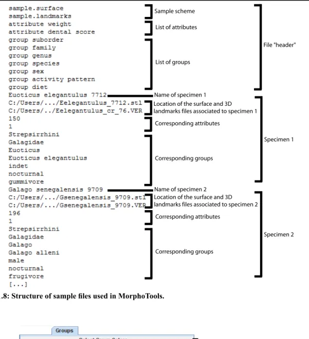
The information related to each specimen (e.g., age, sex, weight, diet, landmark data…) is specified in a sample file. The format of this file is specific to MorphoTools; an example is presented in Figure 1.8. The sample file begins with a list of attributes (continuous variables) and groups (categorical variables). This is followed by a list of specimens and their specific groups/attributes. Once groups are defined in the sample file, they cannot be modified in the application. Such groups are referred to as “static groups”. Static groups can be directly used in the analyses, but a buffering system is designed to allow for the creation of dynamic groups

PCA and CVA filters share the same data types for the input and the output

GLS filter CVA filter XY Plot filter

Schematic VTK pipeline

GLS filter PCA filter XY Plot filter

PC2: 15.7%

PC1: 28.09%

CV2

CV1

Figure 1.7: Interchangeability of processing objects in a pipeline. Processing objects that share the same data types for the input and output are interchangeable. Here, a Principal Component Analysis (PCA) fil-ter is exchanged with a canonical variate analysis (CVA) Filfil-ter. The other elements of the pipeline remain unchanged.

The first group that is selected controls the colors

The second group that is selected controls the symbols

The colors and symbols associated to a class can be changed manually

This control determines the attribute that will be used in analyses involving regression of shape against scalars

Figure 1.9: Interface dedicated to the definition of the dynamic group and attribute selection. Sample scheme

List of attributes

List of groups

File "header"

Location of the surface and 3D landmarks files associated to specimen 1

Corresponding attributes Corresponding groups Name of specimen 1 Specimen 1 Name of specimen 2 Specimen 2 Location of the surface and 3D

landmarks files associated to specimen 2 Corresponding attributes

Corresponding groups

in order to allow more flexibility. The principle of this buffering system is explained with an example (Figure 1.9). First, two groups must be selected. In the example shown in Figure 1.9, the two selected groups are “diet” and “activity pattern”. Each class of the first group is as-sociated with one color (e.g., all the nocturnal specimens are drawn in black), and the classes of the second group are associated with symbols (e.g., all the insectivores are represented by squares). The association of a color and a symbol defines one dynamic group in the application: groups defined using this association are ultimately used in the analyses requiring group defini-tions. In the stated example, all nocturnal insectivores will form a group that is represented by black squares. Furthermore, groups can be merged: it is possible to manually change the color or the symbols associated with one class. For instance, it would also be possible to associate the folivore specimens to the color black. In this case, all nocturnal insectivores and nocturnal folivores would be represented by black squares and would form a group (see again Figure 1.9). The names of the individuals also form a static group. Thus, they can be used to define any pos-sible dynamic group, provided that the names defined in the sample file are unique identifiers of the specimens. In the group scheme, there is a close connection between colors, symbols and groups. Dynamic groups form part of the input of all the analysis processing objects that require the definition of groups (e.g., the CVA filter and the filters involving resampling statistics).

Attributes must be chosen from a list (see Figure 1.9). The selected attributes are used in all analyses involving regression of shape against scalars.

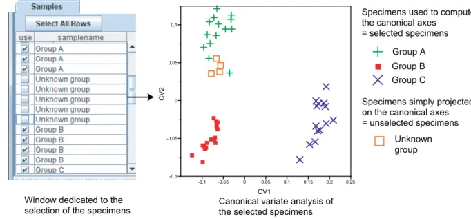
-0,1 -0,05 0 0,05 0,1 C V 2 -0,1 -0,05 0 0,05 0,1 0,15 0,2 0,25 CV1 Group A Group B Group C Unknown group

Specimens used to compute the canonical axes

= selected specimens

Specimens simply projected on the canonical axes = unselected specimens

Window dedicated to the

selection of the specimens Canonical variate analysis of the selected specimens

Figure 1.10: Sample structure used in MorphoTools. Selected specimens form the input of the canonical variate analysis, whereas unselected specimens are simply projected on the resulting canonical axes. Their projecting scores on the axes will serve to classify them in either group A, B or C. In this example, the speci-mens belonging to the “unknown” group are close in shape to the specispeci-mens belonging to group A.

Sample structure 3.2.2

In MorphoTools, each sample is divided into three sub-samples: the selected specimens, the unselected specimens and the mean group specimens.

The first sub-sample contains individuals that were selected from the specimen list. They will be used in all analyses (for instance, they can be used to compute the axes of a PCA). This sub-sample is used most of the time.

The second sub-sample contains all specimens that were not selected from the sample list. As stated above, it might be interesting to discard some specimens because they may distort the results of an analysis. However, it may still be interesting to assess where they would be positioned within the scatter data of a given sample. In MorphoTools, non-selected specimens do not play an active part in an analysis: for instance, they are not used during the computation of the axes of a PCA. The important point is that, optionally, they can be projected a posteriori on these axes. This option is used in association with classification procedures, which assess the morphological affinities that a specimen of special interest (e.g., a fossil) shares with an a priori sample of specimens. The entire procedure works as follows: individuals for which a classification is well-established are first selected as the input of a CVA. The specimens for which the morphological affinities have to be established remain unselected, are projected on the canonical axes (see Figure 1.10) and are classified a posteriori according to their CVA scores

Two groups control the creation of mean group specimens

List of the resulting mean group specimens

Specific controls allow for the manual modification of color and symbols associated to one mean group specimen

Figure 1.11: Interface dedicated to the creation of the mean group sample. First, two groups are selected in the combo-boxes. The different classes associated with each group are combined to define the mean group specimens. In this example, for instance, one of the mean individuals will be the mean of all insectivore lorisids.