Uniqueness of limit cycles for a class of planar vector fields

RESEARCH OUTPUTS / RÉSULTATS DE RECHERCHE

Author(s) - Auteur(s) :

Publication date - Date de publication :

Permanent link - Permalien :

Rights / License - Licence de droit d’auteur :

Bibliothèque Universitaire Moretus Plantin

Institutional Repository - Research Portal

Dépôt Institutionnel - Portail de la Recherche

researchportal.unamur.be

University of Namur

Uniqueness of limit cycles for a class of planar vector fields

Carletti, Timoteo

Published in:

Qualitative Theory of Dynamical Systems

Publication date:

2005

Document Version

Early version, also known as pre-print

Link to publication

Citation for pulished version (HARVARD):

Carletti, T 2005, 'Uniqueness of limit cycles for a class of planar vector fields', Qualitative Theory of Dynamical

Systems, vol. 6, no. 1, pp. 31-43.

General rights

Copyright and moral rights for the publications made accessible in the public portal are retained by the authors and/or other copyright owners and it is a condition of accessing publications that users recognise and abide by the legal requirements associated with these rights. • Users may download and print one copy of any publication from the public portal for the purpose of private study or research. • You may not further distribute the material or use it for any profit-making activity or commercial gain

• You may freely distribute the URL identifying the publication in the public portal ?

Take down policy

If you believe that this document breaches copyright please contact us providing details, and we will remove access to the work immediately and investigate your claim.

Uniqueness of limit cycles for a class of planar vector fields.

Timoteo Carletti

Scuola Normale Superiore, piazza dei Cavalieri 7, 56126 Pisa, Italy

E-mail: t.carletti@sns.it

We give sufficient conditions to ensure uniqueness of limit cycles for a class of planar vector fields. We also exhibit a class of examples with exactly one limit cycle.

Key Words: planar vector fields, uniqueness of limit cycles, Li´enard–like systems

1. INTRODUCTION

In this paper we consider the problem of determine the number of limit cycles, i.e. isolated closed trajectories, for planar vector fields. This is a classical problem, included as part of the XVI Hilbert’s problem. The literature is huge and still growing, for a review see [3] and the more re-cent [6, 5].

An important subproblem is to study systems with a unique limit cycle, in fact in this case the dynamics of the cycle can “dominate” the global dynamics of the whole system. Let us consider planar vector fields of the form:

˙x = β(x) [φ(y) − F (x, y)] , ˙y = −α(y)g(x) , (1) under the regularity assumptions (to ensure the existence and uniqueness of the Cauchy initial problem) for which there exists: −∞ ≤ a < 0 < b ≤ +∞, such that:

A1) β ∈ Lip (a, b) and α ∈ Lip (R);

A2) φ ∈ Lip (R), g ∈ Lip (a, b) and F ∈ C1_{((a, b) × R).}

Without loss of generality we can assume α and β to be positive in their respective domains of definition, in fact the existence of x0such that

β(x0) = 0 (or y0s.t. α(y0) = 0), gives rise to invariant lines, which cannot

intersect a limit cycle. Hence we can reparametrize time, by dividing the vector field by: α(y)β(x). The transformed system is:

˙x = ˜φ(y) − ˜F (x, y), ˙y = −˜g(x) , (2) where ˜φ(y) = φ(y)/α(y), ˜F (x, y) = F (x, y)/α(y) and ˜g(x) = g(x)/β(x). In

the following we will drop out the ˜–mark and consider the general system of previous type.

These systems can be though as “non–Hamiltonian perturbations” of Hamiltonian ones, with Hamilton function: H(x, y) = Φ(y) + G(x), where Φ(y) =R₀yφ(s) ds and G(x) =R₀xg(s) ds, being F (x, y) the “perturbation”.

One can also consider (2) as “generalized” Li´enard equations: ¨

x + f (x) ˙x + g(x) = 0 ,

which in the Li´enard plane can be rewritten as:

˙x = y − F (x), ˙y = −g(x) , (3) where F0_{(x) = f (x), hence our systems generalize (3) by allowing a}

depen-dence of F also on y.

Let λ > 0 and let us consider the energy level Hλ= {(x, y) ∈ R2: Φ(y)+

G(x) = λ}, the knowledge of the flow through Hλ can give informations

about the existence of limit cycles. Because

< ∇Hλ, X(x, y) > ¯ ¯ ¯ Hλ = −F (x, y)g(x) ,

where X(x, y) = (φ(y) − F (x, y), −g(x)), no limit cycles can be completely contained in a region where gF doesn’t change sign. We will see in a while that the set of zeros of F will play a fundamental role in our construction. For Li´enard systems the set of zeros of F is given by vertical lines x = xk

s.t. F (xk) = 0. In a recent paper [2] authors, using ideas taken from

Li´enard systems [1], proved a uniqueness result for systems (2) assuming that F (x, y) vanishes only at three vertical lines x = x− < 0, x = 0 and

x = x+> 0. We generalize this condition by assuming that zeros of F (x, y)

lie on (quite) general curves. More precisely let us assume: B0) F (0, y) = 0 for all real y;

and moreover there exist C1_{functions ψ}

j : R → R, j ∈ {1, 2}, such that1: 1_{We remark that our main result still holds, even if one assume there exist α}

j< 0 < βj, j ∈ {1, 2}, and the functions ψj to be defined in [αj, βj] and verify hypotheses B)

B1) y 7→ ψ1(y), is positive for all y ∈ R, yψ01(y) < 0 for all y 6= 0,

ψ1(0) < b;

B2) y 7→ ψ2(y), is negative for all y ∈ R, yψ02(y) > 0 for all y 6= 0,

ψ2(0) > a;

B3) for all y ∈ R, j ∈ {1, 2}, we have:

F (ψj(y), y) ≡ 0 ,

these curves will be called “non–trivial zeros” of F (x, y) (in opposition with the trivial zeros given by x = 0).

Let us divide the strip (a, b) × R into four distinct domains:

• D> 1 := {(x, y) ∈ (a, b) × R : x > ψ1(y)}; • D< 1 := {(x, y) ∈ (a, b) × R : 0 < x < ψ1(y)}; • D> 2 := {(x, y) ∈ (a, b) × R : ψ2(y) < x < 0}; • D< 2 := {(x, y) ∈ (a, b) × R : x < ψ2(y)}.

The following assumptions generalize “standard sign ones”: C1) yφ(y) > 0 for all y 6= 0 and xg(x) > 0 for all x ∈ (a, b) \ {0}; C2) g(x)F (x, y) < 0 for all (x, y) ∈ D<

1 ∪ D>2.

We remark that hypothesis C2) can be weakened into: C2’) g(x)F (x, y) ≤ 0 for all (x, y) ∈ D<

1 ∪ D>2 except at some (x0, y0)

where strictly inequality holds.

With these hypotheses we ensure that (0, 0) is the only singular point in the strip (a, b) × R of system (2). We are now able to state our main result Theorem 1. Let us consider system (2) and let us assume Hypothe-ses A), B) and C) to hold. Then there is at most one limit cycle which intersects both curves x = ψ1(y) and x = ψ2(y) contained in (a, b) × R,

provided:

D1) the function y 7→ F (x, y)/φ(y) is strictly increasing for (x, y) ∈ D< 1

and y 6= 0;

D2) the function y 7→ F (x, y)/φ(y) is strictly decreasing for (x, y) ∈ D> 2

and y 6= 0;

E) the function x 7→ F (x, y) is positive in D>1, negative in D2< and

increasing in D> 1 ∪ D<2;

F) let Aj(y) = [φ(y)∂xF (x, y) − g(x)∂yF (x, y)]

¯ ¯ ¯ x=ψj(y) , then Aj(y) y > 0 for y 6= 0, j ∈ {1, 2}.

G) there exists a function ζ : [ψ2(0), ψ1(0)] → R such that

φ(ζ(x)) − F (x, ζ(x)) = 0 .

Hypotheses D) and E) naturally generalize hypotheses used in the Li´enard case [1] or in the more general situation studied in [2]. Also hypothesis F) is very natural: each closed trajectory intersects the non–trivial zeros of

F (x, y) at most once in any quadrant. We remark that this condition is

trivially verified if the functions ψjare indentically constant, namely in the

case considered in [2].

The proof of Theorem 1 will be given in the next section. In the last section (§ 3) we will provide a family of systems with exactly one limit cycle. This family is a “natural generalization”of the classical cubic Van der Pol case, thus our result can be considered as a natural extension of this classical existence and uniqueness result.

Acknowledgment I would like to thank the anonymous referee for some

useful remarks allowing me to improve a first version of this paper. 2. PROOF OF THEOREM 1

The aim of this section is to prove our main result Theorem 1. The proof is based on the following remark,

Remark 2. Along any closed curve γ : [0, T ] → (a, b) × R one has:

Z T 0 d dtH ¯ ¯ ¯ flow◦ γ(s) ds = H ◦ γ(T ) − H ◦ γ(0) = 0 ,

moreover if γ is an integral curve of system (2) we can evaluate the inte-grand function to obtain:

Iγ :=

Z T 0

g(xγ(s))F (xγ(s), yγ(s)) ds = 0 , (4)

where γ(s) = (xγ(s), yγ(s)).

The uniqueness result will be proved by showing that the existence of two limit cycles, γ1 contained 2 in γ2, both intersecting x = ψ1(y) and

x = ψ2(y), will imply: Iγ1 < Iγ2, which contradicts (4).

From now on we will assume the existence of two limit cycles, γ1

con-tained in γ2, which intersect both non–trivial zeros of F .

2_{By this we mean γ}

Let us now consider the set of zeros of the equation: φ(y) − F (x, y) = 0 inside D<

1 ∪ D>2. By hypothesis G) this is the graph of some function

x 7→ ζ(x), moreover this function vanishes for x ∈ {ψ2(0), 0, ψ1(0)}, it is

positive for x ∈ (ψ2(0), 0) and negative for x ∈ (0, ψ1(0)).

The sign properties of ζ can be proved as follows. Let ψ2(0) < x < 0,

then by C2) 0 < F (x, ζ(x)) = φ(ζ(x)), using now C1) we conclude that

ζ(x) > 0. The case 0 < x < ψ1(0) can be handle similarly and we omit.

By continuity we get the result about the zeros of ζ(x).

Hypothesis F) guarantees that a closed trajectory can intersect the non– trivial zeros of F (x, y) only once in each quadrant, in fact Aj(y) gives a

measure of the angle between the vector field and the normal to F0 =

{(x, y) : x = ψ1(y)} ∪ {(x, y) : x = ψ2(y)} at (ψj(y), y):

< ∇F0, X(x, y) > ¯ ¯ ¯ F0 = [φ(y)∂xF (x, y) − g(x)∂yF (x, y)] ¯ ¯ ¯ F0 = Aj(y) j ∈ {1, 2} .

For instance, because the angle between the vector field and {(x, y) : x =

ψ1(y)}∩{y > 0} is in absolute value smaller than π/2, a trajectory starting

at (0, ¯y), for some ¯y > 0, which will intersect {(x, y) : x = ψ1(y)}∩{y > 0},

could not meet anew {(x, y) : x = ψ1(y)} ∩ {y > 0}.

From hypotheses D) and the sign of F on D>

2 ∪ D1<, it follows easily

that for all (x, y) ∈ D>

2 ∪ D<1 one has: (y − ζ(x)) (φ(y) − F (x, y)) > 0.

Hence a cycle intersects (D>2 ∪ D1<) ∩ {y > 0} in a region where φ(y) −

F (x, y) > 0, whereas the intersection with (D>2 ∪ D<1) ∩ {y < 0} holds

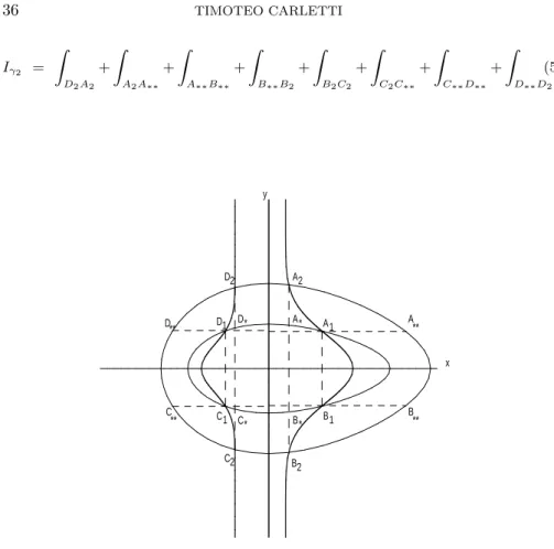
where φ(y) − F (x, y) < 0. This remark allows us to divide the path of integration needed to evaluate Iγj, j ∈ {1, 2}, in two parts: an “horizontal”

one where ˙x > 0 and a “vertical” one, where ˙x vanishes, to be more clear look at Figure 1 where DiAi and BiCi are horizontal arcs, whereas CiDi

and AiBi are vertical ones.

Let us define (see Figure 1), for j ∈ {1, 2}, Aj (respectively Bj) the

intersection point of γj with x = ψ1(y) for y > 0 (respectively y < 0),

and Cj (respectively Dj) the intersection point of γj with x = ψ2(y) for

y < 0 (respectively y > 0). Let also introduce, A∗ being the intersection

point of γ1 and the line x = xA2 contained in the first quadrant, and A∗∗

being the intersection point of γ2 and the line y = yA1 contained in the

first quadrant. Similarly we introduce points: B∗, B∗∗, C∗, C∗∗ and D∗,

D∗∗ (see Figure 1).

According to this subdivision of the arcs of limit cycles, we evaluate Iγj

as follows: Iγ1 = Z D∗A∗ + Z A∗A1 + Z A1B1 + Z B1B∗ + Z B∗C∗ + Z C∗C1 + Z C1D1 + Z D1D∗ ,

Iγ2 = Z D2A2 + Z A2A∗∗ + Z A∗∗B∗∗ + Z B∗∗B2 + Z B2C2 + Z C2C∗∗ + Z C∗∗D∗∗ + Z D∗∗D2 . (5) x y A2 A1 A* A ** B2 B1 B* B** D2 D1 D* D_** C2 C1 C_* C **

FIG. 1. The non–trivial zeros of F (thick), the limit cycles γ1and γ2(thin)

inter-secting both non–trivial zeros of F and their subdivision into arcs.

Let now show that Iγ1 < Iγ2, which prove the contradiction and conclude

the proof.

2.1. Integration along “horizontal arcs”.

Because along horizontal arcs we have ˙x 6= 0, we can change integration variable from t to x, hence for example:

Z DjAj g(x)F (x, y) dt = Z _x Aj x_Dj g(x)F (x, yj(x)) φ(yj(x)) − F (x, yj(x)) dx ,

where yj(x), j ∈ {1, 2}, is the parametrization of γj as graph over x for

Because y2(x) > y1(x) for all x ∈ (xD∗, xA∗), using hypotheses D) and

the sign assumptions C) we get:

g(x)F (x, y1(x)) φ(y1(x)) − F (x, y1(x)) < g(x)F (x, y2(x)) φ(y2(x)) − F (x, y2(x)), hence: Z _x A1 x_D1 g(x)F (x, y1(x)) φ(y1(x)) − F (x, y1(x))dx < Z _xD∗ x_D1 g(x)F (x, y1(x)) φ(y1(x)) − F (x, y1(x))dx+ + Z x_A1 xA∗ g(x)F (x, y1(x)) φ(y1(x)) − F (x, y1(x)) dx + Z x_A2 x_D2 g(x)F (x, y2(x)) φ(y2(x)) − F (x, y2(x)) dx ≤ Z x_A2 x_D2 g(x)F (x, y2(x)) φ(y2(x)) − F (x, y2(x))dx , (6) the last step follows because the integrand function is negative by hy-pothesis C2) and from the previous discussion on the sign of φ(y)−F (x, y).

In a very similar way we can prove that: Z x_C1 x_B1 g(x)F (x, y1(x)) φ(y1(x)) − F (x, y1(x)) dx < Z x_C2 x_B2 g(x)F (x, y2(x)) φ(y2(x)) − F (x, y2(x)) dx . (7)

2.2. Integration along “vertical arcs”.

Along vertical arcs ˙y never vanishes, hence we can perform the integra-tion with respect to the y variable and getting for example:

Z AjBj g(x)F (x, y) dt = Z y_Aj y_Bj F (xj(y), y) dy ,

where xj(y), j ∈ {1, 2}, is the parametrization of γj as graph over y for

y ∈ (yBj, yAj).

Because x2(y) > x1(y) for all y ∈ (yA∗∗, yB∗∗), from hypothesis E) and

the definition of A∗∗ and B∗∗, we get:

Z _y A1 y_B1 F (x1(y), y) dy < Z _yA∗∗ yB∗∗ F (x2(y), y) dy .

Again from the sign assumption on F in D>

1, we get: Z y_A2 yA∗∗ F (x2(y), y) dy > 0 and Z yB∗∗ y_B2 F (x2(y), y) dy > 0 ,

hence we obtain: Z _y A1 y_B1 F (x1(y), y) dy < Z _y A2 y_B2 F (x2(y), y) dy . (8)

Analogously we can prove that: Z _y D1 y_C1 F (x1(y), y) dy < Z _y D2 y_C2 F (x2(y), y) dy . (9)

2.3. Conclusion of the proof.

We are now able to complete our proof. In fact from (6) and (7) of § 2.1, from (8) and (9) of § 2.2 and the subdivision (4) we get:

Iγ1 < Iγ2,

which contradicts (4), and so the Theorem is proved.

3. A SYSTEM WITH EXACTLY ONE LIMIT CYCLE In this last part we present a class of examples exhibiting exactly one limit cycle, which turn out to be a natural generalization, in the case where

F depends on both x and y, of the classical cubic Van der Pol case.

Let us assume that F has the following “special form”:

F (x, y) = x [x − ψ1(y)] [x − ψ2(y)] , (10)

where (ψj)j=1,2 verify hypotheses B). We observe that for this particular

dependence of F on x and y, hypothesis F) is equivalent to the following one:

F’) the function y 7→ Φ(y) + G(ψj(y)) is strictly increasing for positive

y and strictly decreasing for negative ones, j ∈ {1, 2}.

In fact we have:

A1(y) = ψ1(y) [ψ1(y) − ψ2(y)] [φ(y) + g(ψ1(y))ψ01(y)]

= ψ1(y) [ψ1(y) − ψ2(y)]_dyd [Φ(y) + G(ψ1(y))] ,

and the claim follows from the sign properties of ψj and the definitions of

Φ and G. Similarly for A2.

In the rest of the section we will consider the following concrete example given by: φ(y) = y , g(x) = x , ψ1(y) = c1e−d1y 2 + e1and ψ2(y) = −c2e−d2y 2 − e2, (11)

with cj, dj, and ej positive real numbers such that:

(1) c1+ e1= c2+ e2= r,

(2) c1≥ c2 and d1≥ d2,

(3) c1d1max{r, r2} < 1/2.

The remaining part of the section will be devoted to prove the exis-tence of exactly one limit cycle. The proof will be achieved by showing that all, eventually, limit cycles must intersect both non–trivial zeros of F , then proving the existence of at least a limit cycle, we will conclude using Theorem 1.

We left to the reader the easy check that with the above hypotheses, system (11) with F given by (10) satisfies all hypotheses of Theorem 1.

We claim that the vector field is transversal (pointing outward) to the circle Cρ = {(x, y) ∈ R2 : x2+ y2 = ρ2}, with ρ ≤ r = c1+ e1; thus it

can be used as inner boundary of a Poincar´e–Bendixson domain. More-over this circle passes through the points (ψ1(0), 0), (ψ2(0), 0), because

r = ψ1(0) = − ψ2(0), and it lies inside the domain D2>∪ D1< (just

check the curvature of the circle and of the non–trivial zeros of F at these common points, by using (2) and (3)). Hence all orbits, and thus also all eventually limit cycles, must intersect both non–trivial zeros of F .

To conclude it will be enough to prove the existence of at least a limit cycle. To do this we will construct the outer boundary of a Poincar´e– Bendixson domain by using phase–plane comparison techniques. The proof will be divided into three parts, each one considering the regions of phase– plane where pieces of orbits lie.

3.1. Comparing flows for positive x

Let φ0(x) = F (x, 0) = x(x2− r2) and let us compare the flow of the

vector field X, given in coordinates by:

˙x = y − x [x − ψ1(y)] [x − ψ2(y)] , ˙y = −x , (12)

where (ψj(y))j=1,2 are given by (11), with the (Li´enard) vector field X0:

˙x = y − φ0(x), ˙y = −x . (13)

The latter system has [4] one and only one attracting limit cycle, Γ0, (which

intersect both zeros of φ0(x) = 0, i.e. x = ±r). Let γ0(t) be a trajectory of

this vector field lying outside Γ0 (i.e. contained in the unbounded domain

whose boundary is Γ0), passing by the points A = (r0, yA), yA > 0, and

A0= (r0, yA0), yA0< 0, where r

0 _{= r+², for some fixed ² > 0 (see Figure 2).}

Let yA+ yA0= ∆, because the cycle is attracting we have ∆ > 0, a simple

To compare the slopes of the vector fields (12) and (13) we need to estimate F (x, y) − φ0(x) for x > 0; this will be done in the following lemma

Lemma 3. Let F (x, y) = x [x − ψ1(y)] [x − ψ2(y)], where (ψ(y))j=1,2are

given by (11), and let φ0(x) = x(x − ψ1(0))(x − ψ2(0)). Assume moreover

hypotheses (1), (2) and (3) to hold, then:

F (x, y) − φ0(x) > 0 , (14)

for all x > 0 and y ∈ R.

Proof. A direct computation gives:

F (x, y) − φ0(x) = −x2[ψ1(y) + ψ2(y)] + x

£

ψ1(y)ψ2(y) + r2

¤

. (15)

Using the form of (ψj(y))j=1,2 given by (11), the last term in the right

hand side can be rewritten as:

ψ1(y)ψ2(y) + r2 = c1c2 ³ 1 − e−(d1+d2)y2 ´ + c1e2 ³ 1 − e−d1y2 ´ +e1c2 ³ 1 − e−d2y2 ´ ,

thus by the sign assumptions on (cj)j=1,2, (dj)j=1,2 and (ej)j=1,2, we

conclude that this term is always non–negative and zero only for y = 0. Recalling that c1+ e1 = c2+ e2, the remaining term in (15) can be

rewritten as: ψ1(y) + ψ2(y) = −c1 ³ 1 − e−d1y2 ´ + c2 ³ 1 − e−d2y2 ´ ≤ (c1− c2) ³ e−d2y2_{− 1} ´ ≤ 0 ,

where the inequality follows by hypothesis (2). We hence conclude that:

F (x, y) − φ0(x) = −x2[ψ1(y) + ψ2(y)] + x

£

ψ1(y)ψ2(y) + r2

¤

> 0 ,

for all positive x and all y 6= 0

The slope of the vector field (12) is dy dx ¯ ¯ ¯ X = −x

y−F (x,y), whereas the one

for (13) is dy_dx ¯ ¯ ¯ X0 = _y−φ−x

0(x), thus the previous lemma ensures that for x > 0

one has: dy dx ¯ ¯ ¯ X< dy dx ¯ ¯ ¯ X0 , (16)

D₀ 0 A Γ₀ γ 0(t) γ(t) x y A C D B −r r’ A’

FIG. 2. Construction of the outer boundary of a Poincar´e–Bendixson domain. We show the attracting limit cycle of X0, Γ0, and part of one of its orbits from A to A0,

γ0(t) (dotted curves). The dashed curve from C to D0, is a piece of the circle Cr. Solid

curves AB, BC, CD and DA0_{are trajectories of X, γ(t). Arrows denote the vector field} X across the orbit AA0and CD0. BC and DA0are the so–called “horizontal arcs”.

3.2. Comparing flows for negative x

Orbits lying in x < 0 are controled with the following remark. F (x, y) is negative for x < −r and all y ∈ R, thus comparing the flow of X through circles Cρ= {(x, y) ∈ R2: x2+ y2= ρ2}, with ρ > r, we get:

d

dtCρ= −xF (x, y) < 0 x < 0, y ∈ R ,

hence the orbit passing through C = (−r, yC), yC < 0, will reach again

the vertical line x = −r at some D = (−r, yD), yD > 0, and moreover

yD< |yC|.

3.3. Comparing flows for “horizontal arcs”

The following lemma allows us to control “horizontal arcs”of trajectories (see Figure 2):

Lemma 4. The orbit starting at D = (−r, yD), yD > 0, will reach the

y–axis and then the point A0 _{= (r}0_{, y}

A0), y_A0 > 0. Moreover |y_D− y_A0| can

be made as small as we want taking sufficiently large yD.

We observe that a similar result holds for orbits lying in y < 0 connecting

B to C.

3.4. Conclusion of the proof

We are now able to conclude our proof by constructing the outern bound-ary of a Poincar´e–Bendixson domain. Let δ be a positive number such that

δ < ∆/2, where ∆ has been introduced is § 3.1. Assume moreover, see

Lemma 4, that |yD− yA0| < δ and |y_B− y_C| < δ, then we can prove that

orbits of X will approach the origin when winding around it:

yA− yA0 = y_A− y_D+ (y_D− y_A0) > y_A+ y_C− δ

where we used the closeness of yD and yA0 and the relation −y_D > y_C,

moreover

yA+ yC− δ = yA+ yB+ (yC− yB) − δ > ∆ − 2δ > 0 ,

where again we used the closeness of yCand yB. Thus yA−yA0 > 0 and the

construction of an outern Poincar´e–Bendixson boundary is achieved. This allows us to prove the existence of at least one limit cycle, which intersect both curves x = ψj(y), j = 1, 2, hence by Theorem 1 we conclude that this

limit cycle is indeed unique.

In Figure 3 we present a numerical example, to show an application of Theorem 1. y 1 0,5 0 -0,5 -1 x 1 0,5 0 -0,5 -1

FIG. 3. An example with c1 = 0.4, e1 = 0.25, d1 = 0.95, c2 = 0.25, e2 = 0.4,

d2 = 0.75. We numerically compute the attracting unique limit cycle (thick) of X, the

REFERENCES

1. T. Carletti and G. Villari: A note on existence and uniqueness of limit cycles

for Li´enard systems, J. Math. Anal. Appl. 307 (2005), pp. 763–773.

2. M. Sabatini and G. Villari, About limit cycle’s uniqueness for a class of

general-ized Li´enard systems, preprint number 672, Univ. Trento (2004).

3. R. Conti and G. Sansone, Non–linear differential equations, Pergamon Press, (1964).

4. G. Sansone, Sopra l’equazione di Li´enard delle oscillazioni di rilassamento, Ann. Mat. Pura Appl. (4) 28 (1949), pp. 153–181.

5. Ye Yanquia et al., Theory of limit cycles, Trans. Math. Monog., Vol. 66, Americ. Math. Soc., Providence, Rhode Island, (1986).

6. Zhang Zhi-fen et al., Qualitative Theory of differential equations, Trans. Math. Monog., Vol. 101, Americ. Math. Soc., Providence, Rhode Island, (1992).