HAL Id: inserm-00139088
https://www.hal.inserm.fr/inserm-00139088
Submitted on 29 Mar 2007HAL is a multi-disciplinary open access archive for the deposit and dissemination of sci-entific research documents, whether they are pub-lished or not. The documents may come from teaching and research institutions in France or abroad, or from public or private research centers.
L’archive ouverte pluridisciplinaire HAL, est destinée au dépôt et à la diffusion de documents scientifiques de niveau recherche, publiés ou non, émanant des établissements d’enseignement et de recherche français ou étrangers, des laboratoires publics ou privés.
Image analysis by discrete orthogonal Racah moments
Hongqing Zhu Zhu, Huazhong Shu, Jun Liang, Limin Luo, Jean-Louis
Coatrieux
To cite this version:
Hongqing Zhu Zhu, Huazhong Shu, Jun Liang, Limin Luo, Jean-Louis Coatrieux. Image analy-sis by discrete orthogonal Racah moments. Signal Processing, Elsevier, 2007, 87 (4), pp.687-708. �10.1016/j.sigpro.2006.07.007�. �inserm-00139088�
Image Analysis by Discrete Orthogonal Racah Moments
Hongqing Zhu
a, Huazhong Shu
a,c, Jun Liang
a, Limin Luo
a,c, Jean-Louis Coatrieux
b,ca
Laboratory of Image Science and Technology, Department of Computer Science and Engineering,
Southeast University, 210096 Nanjing, People’s Republic of China
b
Laboratoire Traitement du Signal et de l’Image, Université de Rennes I – INSERM U642, 35042
Rennes, France
c
Centre de Recherche en Information Biomédicale Sino-français (CRIBs)
Information about the corresponding author:
Huazhong Shu, Ph. D
Lab. of Image Science and Technology,
Department of Computer Science and Engineering,
Southeast University
People’s Republic of China
Tel: 00-86-25-83794249
Fax: 00-86-25-83794298
Email:
shu.list@seu.edu.cn
HAL author manuscript inserm-00139088, version 1
HAL author manuscript
Abstract
Discrete orthogonal moments are powerful tools for characterizing image shape features for applications in pattern recognition and image analysis. In this paper, a new set of discrete orthogonal moments is proposed, based on the discrete Racah polynomials. In order to ensure numerical stability, the Racah polynomials are normalized, thus creating a set of weighted orthonormal Racah polynomials, to define the so-called Racah moments. This new type of discrete orthogonal moments eliminates the need for numerical approximations. The paper also discusses the properties of Racah polynomials such as recurrence relations and permutability property that can be used to reduce the computational complexity in the calculation of Racah polynomials. Finally, we demonstrate Racah moments’ feature representation capability by means of image reconstruction and compression. Comparison with other discrete orthogonal transforms is performed, and the results show that the Racah moments are potentially useful in the field of image analysis.
Keywords: Discrete orthogonal moments; Racah polynomials; image reconstruction; image compression
1. Introduction
Moments and functions of moments of image intensity values have been widely used in image processing and analysis such as invariant pattern recognition [1], image reconstruction [2], robust line fitting [3], edge detection [4], and image recognition [5]. Among the different types of moments, the Cartesian geometric moments are most widely used due essentially to their simplicity and their explicit geometric meaning. However, the geometric moments are not orthogonal, thus it is difficult to reconstruct the image from them. Teague [6] introduced the Legendre and Zernike moments using the corresponding orthogonal functions as kernels. It was proven that the orthogonal moments possess better image feature representation and are more robust to image noise compared to geometric moments [7]. Since both Legendre and Zernike moments are defined as continuous integrals over a domain of normalized coordinates, the computation of these continuous moments requires a suitable transformation of the image coordinate space and an appropriate approximation of the integrals [8, 9], thus increasing the computational complexity and leading to discretization error. The discrete orthogonal polynomials have been recently introduced in the field of image analysis [10, 11]. Mukundan et al. proposed a set of discrete orthogonal moment functions based on the discrete Tchebichef polynomials for image analysis tasks [10]. More recently, another new set of discrete orthogonal moment functions based on the discrete Krawtchouk polynomials was introduced in [11]. The use of discrete orthogonal polynomials as basis functions for image moments eliminates the need for numerical approximation, and satisfies exactly the orthogonality property in the discrete domain of image coordinate space. This property makes discrete moments superior to the conventional continuous orthogonal moments in terms of image representation capability.
As it is well known, the classical orthogonal polynomials of one discrete variable satisfy a difference equation of hypergeometric type. The discrete orthogonal polynomials can be classified into two categories [12]. The first one is the set of polynomials that are orthogonal on uniform lattice {x = 0, 1, 2,…}. These orthogonal polynomials are solutions of the following difference equation [13]
0
)
(
)
(
)
(
)
(
)
(
x
Δ
∇
p
nx
+
τ
x
Δ
p
nx
+
λ
np
nx
=
σ
(1) whereΔ
p
n(
x
)
=
p
n(
x
+
1
)
−
p
n(
x
)
,∇
p
n(
x
)
=
p
n(
x
)
−
p
n(
x
−
1
)
denote the forward and backward finite difference quotients, respectively.σ
(x
)
andτ
(x
)
are functions of second and first degree respectively,λ
n is an appropriate constant. The discrete Meixner, Krawtchouk, Charlier, Tchebichef, and Hahn polynomials belong to this category. The second one consists of the polynomials being orthogonal on non-uniform lattice {x
=
x
(s
)
, s = 0, 1,2,…}, which satisfy the following difference equation [13, 14]
0
)
(
]
)
(
)
(
)
(
)
(
[
2
)]
(
[
~
]
)
(
)
(
[
)
2
1
(
)]
(
[
~
+
=
∇
∇
+
Δ
Δ
+
∇
∇
−
Δ
Δ
s
y
s
x
s
y
s
x
s
y
s
x
s
x
s
y
s
x
s
x
n n n n nτ
λ
σ
(2)Here
σ
~ x
(
)
andτ
~ x
(
)
are polynomials in x(s) of degree at most two and one, respectively, andλ
n is an appropriate constant. According to different non-uniform lattice functions, we may have different polynomials. For example, for non-uniform latticex
(
s
)
= s
s
(
+
1
)
, we obtain the Racah or dual Hahn polynomials. Forx
(
s
)
=
q
sor
(
q
s−
q
−s)
/
2
, we have the q-Krawtchouk, or q-Meixner, or q-Charlier, or q-Hahn polynomials. For2
/
)
(
)
(
s
q
sq
sx
=
+
− or(
q
is+
q
−is)
/
2
, we have the q-Racah or q-dual Hahn polynomials [12, 13].In recent years, special attention has been paid to the study of the discrete orthogonal polynomials on non-uniform lattice [15-19]. Lattice field theories have become a powerful tool to avoid infinities in perturbative methods, and to obtain exact solutions of the field equations [20, 21]. However, to the best of our knowledge, until now, no discrete orthogonal polynomial defined on non-uniform lattice has been used in the field of image analysis. In this paper, we address this problem by introducing a new set of discrete orthogonal polynomials, namely Racah polynomials, which are orthogonal on non-uniform lattice
x
(
s
)
= s
s
(
+
1
)
. The Racah polynomials introduced by Askey and Wilson contain as limiting cases the classical polynomials of Jacobi, Laguerre and Hermite and their discrete analogues which go under the names of Hahn, Meixner, Krawtchouk and Charlier polynomials [22, 23]. In physics, the Racah coefficients usually arise in atomic and nuclear shell model calculations. In modern mathematics, the Racah polynomials play a leading role in the theory of orthogonal polynomials of discrete variables and of finite difference equations [22].The objective of this paper is to introduce the Racah polynomials into the field of image analysis and attempts to demonstrate their potential usefulness in this field. To achieve this, the Racah polynomials are first scaled to be within the range of [–1, 1], so that the numerical stability of the polynomials can be assumed. The scaled Racah polynomials are then used as basis functions to define a new type of discrete orthogonal moments known as Racah moments. Similar to other discrete orthogonal moments, the error in the computed Racah moments due to discretization does not exist. Image can thus be exactly reconstructed from the complete set of discrete moments.
Although the Racah polynomials are orthogonal on non-uniform lattice, the discrete Racah moments defined
in this paper apply to uniform pixel grid image. The difference between the Racah moments and the discrete moments based on the polynomials that are orthogonal on uniform lattice (e.g., discrete Tchebichef moments and Krawtchouk moments) is that the latter is directly defined on the image grid but, for the former, we should introduce an intermediate, non-uniform lattice,
x
(
s
)
= s
s
(
+
1
)
.The paper is organized as follows: in section 2, we present the Racah polynomials of a discrete variable on non-uniform lattice. This section also provides the definition of weighted Racah polynomials and the Racah moments. Section 3 discusses the recurrence relations and permutability property of Racah polynomials, which can be effectively used in Racah polynomial computation. The comparative study of the proposed approach with some other discrete orthogonal transforms in terms of the image reconstruction and compression capability is performed in Section 4 and concluding remarks are reported in Section 5.
2. Racah moments
2.1. Discrete orthogonal polynomials on non-uniform lattice
Let us first review some general properties of orthogonal polynomials of a discrete variable on non-uniform lattice [13, 24]. As previously indicated, the discrete orthogonal polynomials on non-uniform lattice are solutions of Eq. (2). It is convenient to rewrite Eq. (2) in the following equivalent form.
0
)
(
)
(
)
(
)
(
]
)
(
)
(
[
)
2
1
(
)
(
+
=
Δ
Δ
+
∇
∇
−
Δ
Δ
s
y
s
x
s
y
s
s
x
s
y
s
x
s
n n n nτ
λ
σ
(3) where)
2
1
(
)]
(
[
~
2
1
)]
(
[
~
)
(
s
=
σ
x
s
−
τ
x
s
Δ
x
s
−
σ
(4))]
(
[
~
)
(
s
τ
x
s
τ
=
(5) It is known that for some special kind of lattices, solutions of Eq. (3) are orthogonal polynomials of a discrete variable, i.e., they satisfy the following orthogonality property2 1
)]
2
1
(
)[
(
)
(
)
(
m nm n b a s ns
P
s
s
x
s
d
P
ρ
Δ
−
=
δ
∑
− = (6)where
d
n2 denotes the square of the norm of the corresponding orthogonal polynomials, and ρ(s) is a non-negative function (weighting function), i.e.,
)]
0
2
1
(
)[
(
s
Δ s
x
−
>
ρ
, a ≤ s ≤ b – 1 (7) supported in a countable set of the real line (a, b), and ρ(s) is the solution of the following Pearson-type difference equation [18])
(
)
(
)]
(
)
(
[
)
2
1
(
x
x
x
x
s
x
ρ
τ
ρ
σ
=
−
Δ
Δ
(8)The polynomial solutions of Eq. (3), denoted by
y
n[
x
(
s
)]
≡
P
n(
s
)
, are uniquely determined, up to a normalizing factor Bn, by the difference analogue of the Rodrigues formula [13, 16, 25].)]
(
[
)
(
)
(
( )s
s
B
s
P
n n n n n=
ρ
∇
ρ
,[
(
)]
)
(
)
(
)
(
)]
(
[
1 1 ) (s
s
x
s
x
s
x
s
n n n n n nρ
ρ
∇
∇
∇
∇
⋅⋅
⋅
∇
∇
=
∇
− (9) where)
2
(
)
(
s
x
s
n
x
n=
+
,∏
=+
+
=
n k ns
n
s
s
k
1)
(
)
(
)
(
ρ
σ
ρ
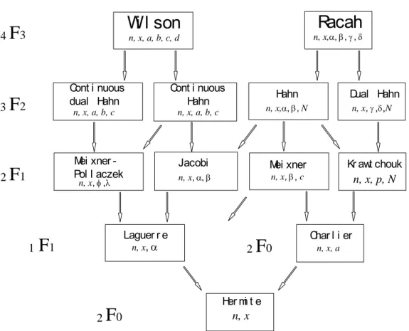
(10) In this paper, we select Racah polynomials as basis functions to define the new moments because all other polynomial families in Askey scheme (e.g., Krawtchouk, Meixner, Laguerre, Charlier, and Hermite polynomials) can be derived from the Racah polynomials by taking suitable limits [23]. Fig. 1 shows examples for which limit relations between neighboring polynomials are available, many other limit relations about the hypergeometric orthogonal polynomials and their q-analogues can be found in [22].2.2. Racah polynomials
The classical Racah polynomials
u
n( , )(
s
,
a
,
b
)
β α
, n = 0, 1, …, L–1, defined on non-uniform lattice x(s) = s(s+1), are solutions of Eq. (3) corresponding to [13]:
)
1
(
)
(
)
2
(
)
1
)(
1
(
)
(
)
1
(
)
(
)
1
(
)
(
)
)(
)(
)(
(
)
(
+
+
+
=
+
+
−
+
+
−
+
+
+
−
+
=
−
+
−
+
+
−
=
n
n
s
x
b
b
a
a
s
s
b
a
s
b
s
a
s
s
nα
β
λ
β
α
β
α
α
β
β
α
τ
α
β
σ
(11)and the weighting function ρ(s) is given by
)
1
(
)
(
)
1
(
)
1
(
)
1
(
)
(
)
1
(
)
1
(
)
(
+
+
Γ
−
Γ
+
−
Γ
+
+
−
Γ
+
+
+
Γ
−
+
Γ
+
+
−
Γ
+
+
Γ
=
s
b
s
b
a
s
s
a
s
b
s
b
a
s
s
a
s
β
α
α
β
ρ
(12)where the parameters a, b, α and β are restricted to
b
a
<
<
− 2
1
/
,α
>
−
1
,−
1
<
β
<
2
a
+
1
,b
=
a
+
N
(13) Here N × N is the size of the image.
The n-th order Racah polynomial
u
n( , )(
s
,
a
,
b
)
β α
is defined explicitly as generalized hypergeometric sums [26]:
⎟⎟
⎠
⎞
⎜⎜
⎝
⎛
+
+
+
−
+
+
+
+
−
+
+
+
−
×
+
+
+
+
+
−
=
;
1
1
,
1
,
1
1
,
,
1
,
)
1
(
)
1
(
)
1
(
!
1
)
,
,
(
4 3 ) , (α
β
β
α
α
β
β αb
a
b
a
s
a
s
a
n
n
F
b
a
b
a
n
b
a
s
u
n n n n , n = 0, 1, …, L – 1, s = a, a + 1, …, b – 1, (14) where (u)k is the Pochhammer symbol defined as
)
(
)
(
)
1
(
)
1
(
)
(
u
k
u
k
u
u
u
u
kΓ
+
Γ
=
−
+
+
=
"
(15) and 4F
3(
⋅
)
is the generalized hypergeometric function given by
!
)
(
)
(
)
(
)
(
)
(
)
(
)
(
)
;
,
,
;
,
,
,
(
0 1 2 3 4 3 2 1 3 2 1 4 3 2 1 3 4k
z
b
b
b
a
a
a
a
z
b
b
b
a
a
a
a
F
k k k k k k k k k∑
∞ ==
(16) The Racah polynomials Rn(x(x + γ + δ + 1); α, β, γ, δ) defined in [22] can be obtained by identifying the parameterα, β, x, γ and δ with our β, α, s – a, a + b + α, a – b – α, respectively, and multiplying
u
n(α,β)(
s
,
a
,
b
)
byn n n
a
b
b
a
n
!
(
1
)
(
1
)
(
1
)
1
−
+
β
+
+
+
α
+
.Note that if we take γ + 1 = –N and let
δ
→
∞
in Rn(x(x + γ + δ + 1); α, β, γ, δ), we obtain the Hahnpolynomials Qn(x; α, β, N). If we take α = pt and β = (1–p)t in the Hahn polynomials and let t → ∞, we obtain the
Krawtchouk polynomials Kn(x; p, N) [22]. Setting α = 0 and β = 0, the Hahn polynomials reduce to the Tchebichef
polynomials [13].
The Racah polynomials satisfy the following orthogonality property
2 1 ) , ( ) , (
)]
2
1
(
)[
(
)
,
,
(
)
,
,
(
nm n b a s m ns
a
b
u
s
a
b
s
x
s
d
u
αβ αβρ
Δ
−
=
δ
∑
− = , n, m = 0, 1,…, L – 1 (17) with)
(
)
1
(
)!
1
(
!
)
1
2
(
)
1
(
)
1
(
)
1
(
)
1
(
2n
b
a
n
n
a
b
n
n
n
b
a
n
a
b
n
n
d
n−
−
+
Γ
+
+
+
Γ
−
−
−
+
+
+
+
+
+
+
Γ
+
+
+
+
−
Γ
+
+
Γ
+
+
Γ
=
β
β
α
β
α
α
β
α
β
α
, n = 0, 1, …, L – 1 (18)The set of Racah polynomials is not suitable for defining moments because the range of values of the polynomials expands rapidly with the increase of the order. A usual method to avoid numerical fluctuations for moment
computations is by means of normalization. We define the weighted Racah polynomials in the following subsection.
2.3. Weighted Racah polynomials
To avoid numerical instability in polynomial computation, the Racah polynomials are normalized by utilizing the square norm and the weighting function. The set of weighted Racah polynomials is defined as
)]
2
1
(
[
)
(
)
,
,
(
)
,
,
(
ˆ
2 ) , ( ) , (=
Δ
−
s
x
d
s
b
a
s
u
b
a
s
u
n n nρ
β α β α n = 0, 1, …, L – 1 (19)In this case, the orthogonality condition given by Eq. (17) becomes
nm b a s m n
s
a
b
u
s
a
b
u
αβ αβ=
δ
∑
− = 1 ) , ( ) , ()
,
,
(
ˆ
)
,
,
(
ˆ
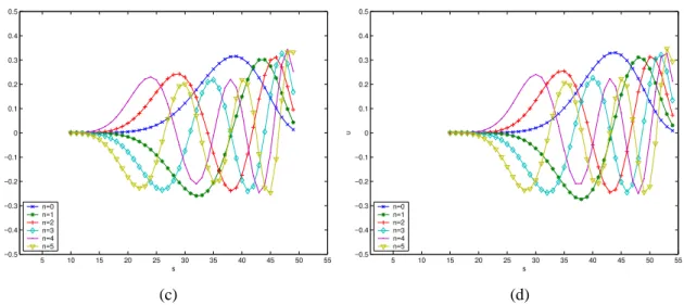
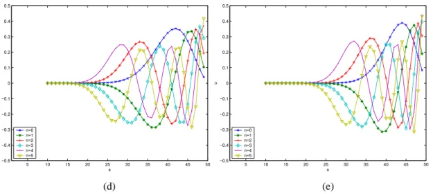
n, m = 0, 1, …, L – 1 (20)where variable s has a uniform step s = a, a+1, … , b–1. The values of the weighted Racah polynomials are thus confined within the range of [–1, 1]. Figs. 2 and 3 show the plots for the first few orders of the weighted Racah polynomials with different choices of parameter values.
2.4. Racah moments
Racah moments are a set of moments formed by using the weighted Racah polynomials. The one-dimensional (1-D) Racah moments is defined as
∑
− ==
1 ( , ))
(
)
,
,
(
ˆ
b a s n nu
s
a
b
f
s
v
αβ n = 0, 1, …, L – 1 (21)where f(s) is 1-D signal with length N. If a set of Racah moments
v
n up to order M is given, the Racah moment-based signal reconstruction is as follows:∑
=≈
M n n nu
s
a
b
v
s
f
0 ) , ()
,
,
(
ˆ
)
(
αβ , s = a, a + 1, …, b – 1 (22) Similar to 1-D signal reconstruction, given an image f(s, t) with size N × N, the (n + m)-th order Racah moment is defined as)
,
(
)
,
,
(
ˆ
)
,
,
(
ˆ
1 1 ) , ( ) , (t
s
f
b
a
t
u
b
a
s
u
U
b a s b a t m n nm∑∑
− = − ==
αβ α β n, m = 0, 1, …, L – 1 (23)The orthogonality property of Racah polynomials helps in expressing the image intensity function f (s, t) in terms of
its Racah moments. Reconstructed image can be obtained by using the following inverse Racah moment transform:
∑∑
− = − ==
1 0 1 0 ) , ( ) , ()
,
,
(
ˆ
)
,
,
(
ˆ
)
,
(
L n L m m n nmu
s
a
b
u
t
a
b
U
t
s
f
αβ αβ , s, t = a, a + 1, …, b – 1 (24) where (s, t) represents the uniform pixel grid of image.When only moments of order up to M are used, the image intensity function f (s, t) is approximated by
∑∑
= ==
M n M m m n nmu
s
a
b
u
t
a
b
U
t
s
f
0 0 ) , ( ) , ()
,
,
(
ˆ
)
,
,
(
ˆ
)
,
(
~
αβ αβ , s, t = a, a + 1, …, b – 1 (25)3. Computational aspects of Racah moments
In this section, we discuss the computational aspects of Racah moments. We present some properties of Racah polynomials including the recurrence relations with respect to n and s. The Wigner 6j symbols are used to obtain the permutability property about n + a and s. These properties can be effectively used to compute the polynomial values.
3.1. Recurrence relation with respect to n
The computation of Racah polynomials based on hypergeometric and gamma functions is very expensive. To remedy this problem, the following recurrence relation of the weighted Racah polynomials is used.
)
,
,
(
ˆ
)
,
,
(
ˆ
)
,
,
(
ˆ
( , ) 2 2 ) , ( 1 1 ) , (b
a
s
u
d
d
C
b
a
s
u
d
d
B
b
a
s
u
A
n n n n n n n n n n β α β α β α − − − −+
=
(26) where)
2
)(
1
2
(
)
(
n
n
n
n
A
n+
+
−
+
+
+
+
=
β
α
β
α
β
α
(27)
)
2
)(
2
2
(
2
]
)
2
/
(
)
2
/
)[(
(
8
)
2
)(
2
2
(
4
2
)
(
)
(
2 2 2 2 2 2 2 2n
n
a
b
n
n
b
a
b
a
x
B
n+
+
−
+
+
−
−
+
−
−
+
+
−
+
+
+
−
+
+
−
+
+
−
=
β
α
β
α
β
α
α
β
β
α
β
α
α
β
(28)⎥
⎥
⎦
⎤
⎢
⎢
⎣
⎡
⎟
⎠
⎞
⎜
⎝
⎛
−
+
+
−
⎟
⎠
⎞
⎜
⎝
⎛
−
+
+
×
⎥
⎥
⎦
⎤
⎢
⎢
⎣
⎡
⎟
⎠
⎞
⎜
⎝
⎛
−
+
+
−
⎟
⎠
⎞
⎜
⎝
⎛
+
+
−
−
+
+
−
+
+
−
+
−
+
−
=
2 2 2 22
1
2
2
1
2
)
1
2
)(
2
2
(
)
1
)(
1
(
β
α
β
α
β
α
β
α
β
α
β
α
β
α
n
a
b
n
b
a
n
n
n
n
C
n(29) with
)]
2
1
(
[
)
(
)
,
,
(
ˆ
2 0 ) , ( 0=
Δ
x
s
−
d
s
b
a
s
u
αβρ
(30))]
2
1
(
[
)
(
)
2
/
1
(
)
2
/
1
(
)
1
(
)
(
)
(
1
)
,
,
(
ˆ
2 1 1 1 ) , ( 1+
−
−
Δ
−
−
−
−
=
x
s
d
s
s
x
s
x
s
s
s
b
a
s
u
ρ
ρ
ρ
ρ
β α (31)3.2. Recurrence relation with respect to s
The recurrence relation of discrete Racah polynomials with respect to s can be derived from Eq. (3) as follows:
)
,
,
2
(
)]
1
(
)
1
2
(
)
1
(
)[
1
(
)
1
(
)
,
,
1
(
)]
1
(
)
1
2
(
)
1
(
)[
1
(
)]
1
(
2
)
1
(
)
1
(
)
1
(
)[
1
2
(
)
,
,
(
) , ( ) , ( ) , (b
a
s
u
s
s
s
s
s
s
b
a
s
u
s
s
s
s
s
s
s
s
s
s
b
a
s
u
n n n−
−
−
+
−
−
−
⋅
−
−
−
−
+
−
−
−
⋅
−
−
−
+
−
−
=
β α β α β ατ
σ
σ
τ
σ
λ
τ
σ
(32)To obtain the starting values, we rewrite ( )
[
n(
s
)]
n n
ρ
∇
defined by Eq. (9) for Racah polynomials as [18])
(
)
2
/
)
1
(
(
)
2
/
1
(
)!
(
!
!
)
1
(
)]
(
[
0 0 ) (l
s
l
m
s
x
l
s
x
l
n
l
n
s
n n m n n n l l n n n−
−
+
−
∇
+
−
∇
×
−
−
=
∇
∏
∑
= =ρ
ρ
(33)Using Eq. (33), we have
!
)
0
(
)
0
(
) (n
n n n nρ
ρ
=
∇
(34))
0
(
)!
2
(
)
1
(
)
1
(
)!
2
(
2
)
1
(
) ( n n n n nn
n
n
n
ρ
ρ
ρ
+
+
−
+
=
∇
(35) thus n n n n n na
a
b
b
n
n
b
a
u
(
1
)
(
1
)
(
1
)
(
)
)
!
(
)
1
(
)
,
,
0
(
2 ) , (αβ=
−
+
β
−
+
+
α
+
−
(36))
,
,
0
(
]
2
)
1
(
)
0
(
)
1
(
[
)
1
(
)
0
(
)
1
)(
2
(
2
)
,
,
1
(
( , ) ) , (b
a
u
n
n
n
n
b
a
u
n n n n β α β αρ
ρ
ρ
ρ
−
+
+
+
=
(37)We obtain the recurrence relation for the weighted Racah polynomials with respect to s
)
,
,
2
(
ˆ
)
3
2
)(
2
(
)]
2
1
(
)[
(
)]
1
(
)
1
2
(
)
1
(
)[
1
(
)
1
(
)
,
,
1
(
ˆ
)
1
2
)(
1
(
)]
2
1
(
)[
(
)]
1
(
)
1
2
(
)
1
(
)[
1
(
)]
1
(
2
)
1
(
)
1
(
)
1
(
)[
1
2
(
)
,
,
(
ˆ
) , ( ) , ( ) , (b
a
s
u
s
s
s
x
s
s
s
s
s
s
s
b
a
s
u
s
s
s
x
s
s
s
s
s
s
s
s
s
s
s
b
a
s
u
n n n−
−
−
−
−
−
+
−
−
−
⋅
−
−
−
−
−
−
−
+
−
−
−
⋅
−
−
−
+
−
−
=
β α β α β αρ
ρ
τ
σ
σ
ρ
ρ
τ
σ
λ
τ
σ
Δ
Δ
n = 0, 1, …, L – 1, s = 2, 3, …, b – 1 (38) where 2 2 ) , ((
0
)
)
(
)
1
(
)
1
(
)
1
(
)
!
(
)
1
(
)
,
,
0
(
ˆ
n n n n n n nd
n
b
b
a
a
n
b
a
u
αβ=
−
+
β
−
+
+
α
+
−
ρ
(39))
,
,
0
(
ˆ
)
0
(
)
1
(
3
2
)
1
(
)
0
(
)
1
(
)
1
(
)
0
(
)
1
)(
2
(
2
)
,
,
1
(
ˆ
( , ) ( , )b
a
u
n
n
n
n
b
a
u
n n n n β α β αρ
ρ
ρ
ρ
ρ
ρ
⎥
⎦
⎤
⎢
⎣
⎡
−
+
+
+
=
(40) with)
1
(
)
(
)
1
(
)
1
(
)
1
(
)
(
)
1
(
)
1
(
)
(
+
+
Γ
−
−
Γ
+
−
Γ
+
+
−
Γ
+
+
+
+
Γ
−
+
Γ
+
+
+
−
Γ
+
+
+
Γ
=
s
b
n
s
b
a
s
s
a
n
s
b
s
b
n
a
s
n
s
a
s
nβ
α
α
β
ρ
(41)Using Eq. (39), we obtain
)
,
,
0
(
ˆ
)
)(
)(
)(
(
1
)
,
,
0
(
ˆ
( , ) 1 1 2 ) , (b
a
u
d
d
n
b
n
b
n
a
n
a
n
b
a
u
n n n n β α β αβ
α
− −−
+
+
+
−
+
−
=
(42)The above equations can be used to effectively compute the weighted Racah polynomial values.
3.3. Permutability property about n+a and s
The permutability property can be used to reduce the time required for computing the Racah polynomials. In this subsection, we discuss the permutability property of weighted Racah polynomials for some special cases of parameters a, α and β. To demonstrate the permutability property, we need to utilize the concept of Wigner 6j symbols introduced by Wilson and Askey [27, 28]. The Wigner 6j symbols are related to the coefficients of transformations between different coupling schemes of three angular momenta j1, j2, j3, and they are defined in terms of the
hypergeometric function as [28]
( )
⎟⎟
⎠
⎞
⎜⎜
⎝
⎛
+
+
+
−
−
+
−
+
−
+
+
−
−
−
+
+
−
−
−
×
−
+
−
+
+
+
−
×
⎥
⎦
⎤
⎢
⎣
⎡
−
+
+
−
+
+
+
−
+
+
+
+
+
−
+
−
+
−
×
⎥
⎦
⎤
⎢
⎣
⎡
−
+
+
−
+
+
+
−
+
+
+
+
+
−
+
−
+
−
−
=
⎭
⎬
⎫
⎩
⎨
⎧
+ + +1
;
2
2
,
1
1
,
,
1
,
)!
)(
1
(
)!
2
(
)!
(
)!
(
)!
1
(
)!
(
)!
1
(
)!
(
)!
(
)!
(
)!
(
)!
(
)!
1
(
)!
(
)!
1
(
)!
(
)!
(
)!
(
1
3 2 1 2 3 2 1 23 2 3 23 2 3 12 2 1 12 2 1 3 4 3 2 1 3 2 1 2 2 / 1 23 2 3 2 3 23 23 2 3 1 23 23 1 23 1 23 1 23 2 3 2 / 1 12 2 1 2 12 12 2 1 3 12 12 3 12 3 3 12 12 2 23 3 12 2 1 1 12 23j
j
j
j
j
j
j
j
j
j
j
j
j
j
j
j
j
j
j
j
j
F
j
j
j
j
j
j
j
j
j
j
j
j
j
j
j
j
j
j
j
j
j
j
j
j
j
j
j
j
j
j
j
j
j
j
j
j
j
j
j
j
j
j
j
j
j
j
j
j
j
j
j
j
j
j
j
j
j
j
j
j
j
j
j
j j j j (43)The Wigner 6j symbols are associated to the weighted Racah polynomials through the following relation [12, 26]
⎭
⎬
⎫
⎩
⎨
⎧
+
+
−
=
+ + 23 3 12 2 1 2 1 23 12 ) ( ) , ()]
1
2
)(
1
2
[(
)
1
(
)
,
,
(
ˆ
1 23j
j
j
j
j
j
j
j
b
a
s
u
nαβ j j j (44) where2
1
,
2
1
,
2
1
2
1
,
,
2
3 2 1 23 12−
+
=
−
−
=
−
−
+
+
=
−
−
+
+
=
=
+
+
=
b
a
j
a
b
j
a
b
j
b
a
j
s
j
n
j
β
α
β
α
β
α
(45)Eq. (44) can be rewritten as
) ( 23 3 12 2 1 2 1 23 12 ) 4 ( ) ( 23 3 12 2 1 2 1 23 12 ) ( ) ( ) , ( 23 12 1 23 12 23 12 1 23 12 1 23 1
)
1
/(
)]
1
2
)(
1
2
[(
)
1
(
)
1
(
)
1
/(
)]
1
2
)(
1
2
[(
)
1
(
)
,
,
(
ˆ
j j j j s j j j j j j j j j j j j j j nj
j
j
j
j
j
j
j
j
j
j
j
j
j
j
j
b
a
s
u
+ + + + + + + + + + + + + +−
⎭
⎬
⎫
⎩
⎨
⎧
+
+
−
−
=
−
⎭
⎬
⎫
⎩
⎨
⎧
+
+
−
=
β α (46)Let a = α = β in Eq. (45), we have
s
j
a
n
j
a
j
j
j
j
j
=
1=
3,
2=
−
,
12=
+
,
23=
, (47)It can be derived from Eqs. (46) and (47) that
⎪⎩
⎪
⎨
⎧
+
+
−
=
− −even
is
if
),
,
,
(
ˆ
odd
is
if
),
,
,
(
ˆ
)
,
,
(
ˆ
) , ( ) , ( ) , (s
b
a
a
n
u
s
b
a
a
n
u
b
a
s
u
a s a s n αβ β α β α , n = 0, 1, …, L – 1, s = a, …, b – 1 (48)Note that the above relation is only valid for the special case where a = α = β. This property can be used to reduce the number of arithmetic operations in the computation of Racah polynomial values by half.
4. Experimental results and discussions
This section presents a set of test images to validate the effectiveness of the proposed method. A comparative
study of the Racah moments in terms of the image reconstruction and compression capability with Legendre, Tchebichef and Krawtchouk moments and the discrete cosine transform (DCT) is performed.
4.1. Image reconstruction
We first illustrate the influence of the parameters a, b, α and β on image reconstruction when using the Racah moments. According to the constraints imposed on these parameters given by Eq. (13), we have systematically chosen the parameters as a = α and b = a + N in all the experiments where N × N is the image size. In the first example, we consider the case where a = α = β. In this case, for a given value of N, only the parameter a is adjustable. Fig. 2 shows the plots of the first few orders of Racah polynomials for N = 40 with different values of a. From this figure, we can observe that the Racah polynomials contract and move from left to right as a increases. We use a binary Chinese character whose size is 40 × 40 pixels as original image to test the influence of the parameter a on the reconstruction results. Four cases have been tested: (a) a = α = β = 0, and b = 40; (b) a = α = β = 5, and b = 45; (c) a = α = β = 10, and b = 50; (d) a = α = β = 15, and b = 55. Fig. 4 shows the original image and the reconstructed results under different choices of parameter a with moment order up to 2, 10, 20, and 35, respectively. The following mean square error ε is used to measure the accuracy of the reconstructed images.
∑∑
− = − =−
=
1 1 2 2(
,
)]
~
)
,
(
[
1
b a s b a tt
s
f
t
s
f
N
ε
(49) where f (s, t) and ~f (s,t)denote the original image and the reconstructed image, respectively.The plot of corresponding reconstruction errors is depicted in Fig. 5. From Figs. 4 and 5, it can be seen that the difference between the reconstructed images is relatively important when only the moments of lower order are used. Conversely, when the maximum order of moments is high (M ≥ 25), the reconstruction errors with different values of parameter a are almost the same.
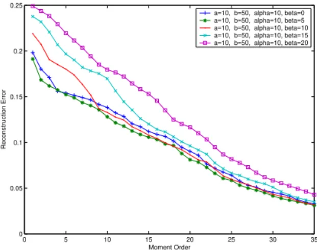
In the second example, we consider the case where α ≠ β. We discuss the influence of parameter β on the reconstructed results. A constant value is assigned to the parameter a, we set a = α = 10 for this example. Five cases have been tested according to constraints given by Eq. (13): (a) β = 0; (b) β = 5; (c) β = 10; (d) β = 15; (e) β = 20. Fig. 3 depicts the plots of Racah polynomials with different values of β with N = 40. We can observe from Fig. 3, similarly to Fig 2, the contraction and shift of Racah polynomials as β increases.
As for the previous example, we present the reconstructed results and corresponding errors in Figs. 6 and 7,
respectively. It can be seen that the second choice, i.e., a = α = 10, b = 50 and β = 5, gives the best reconstructed results among all the test cases. The results obtained with third set (a = α = 10, b = 50 and β = 10) is comparable to those obtained with the second test case. We think this is because the weighted Racah polynomials, with these two choices of parameters, are approximately situated at the middle of the region of definition (see Figs. 3(b) and (c)), so that the emphasis of the moments will be at the center of the image. It can also be seen for the last test case, that the reconstruction begins from bottom right corner. Note that the other choices (β = 4 and β = 6) have also been tested for this example, but the reconstruction results are very similar to those with β = 5.
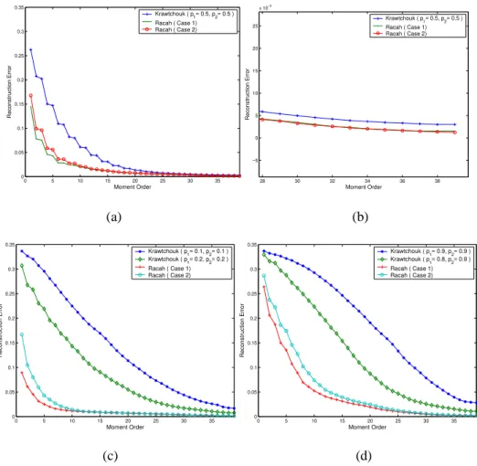
As indicated by Yap et al. [11], the Krawtchouk moments can be used to extract the feature of an image by adjusting the parameter p. The Racah moments share a similar characteristic exemplified hereafter. We apply both Krawtchouk and Racah moments to reconstruct a gray-level image whose size is 40×40. Fig. 8 shows the results of image reconstruction by using different values of p1 and p2 for Krawtchouk moments, and different values of a, b, α
and β for Racah moments. It can be visually seen from this figure that for Krawtchouk moments, the parameter p1 can
be used to shift the region-of-interest (ROI) horizontally: if p1 < 0.5, the shifting of the ROI is to the left, while p1 >
0.5, it shifts the ROI to the right. The parameter p2 shifts the ROI vertically: if p2 < 0.5, the ROI is shifted to the top,
while p2 > 0.5, the ROI is shifted to the bottom. This is consistent with the results obtained by Yap [11]. For Racah
moments, for a fixed value of a, the parameter β controls the shifting of the ROI: the smaller the value of β, the emphasis of the ROI on the top left corner will be. Conversely, the ROI of the image shifts to the bottom right corner when β takes greater value. Fig. 9 depicts the reconstruction errors for both methods. It can be observed that the choice of the parameter β corresponding to the case where the emphasis of the moments is at the center of the image gives the best reconstruction result. Based on the above test results, we found that when the wave crest of zero order curves of Racah polynomials is close to the middle value of interval [a, b], we could obtain the best reconstructed image. This is the reason why we use such a choice of parameters a, b, α and β in the following examples.
In the fourth example, we compare the performance of the proposed Racah moments (RM) with Legendre moments (LM), Tchebichef moments (TM) and Krawtchouk moments (KM) and the well-known discrete cosine transform (DCT). The 2D discrete DCT transform of a N×N image is defined by [29]
∑∑
− = − = + + = 1 0 1 0 2 ) 1 2 ( cos 2 ) 1 2 ( cos ) , ( ) ( ) ( ) , ( N s N t N m t N n s t s f m c n c m n F π π , n, m = 0, 1,…, N – 1 (50) with⎪⎩
⎪
⎨
⎧
=
=
otherwise
,
2/
0
if
,
/
1
)
(
N
n
N
n
c
,⎪⎩
⎪
⎨
⎧
=
=
otherwise
,
2/
0
if
,
/
1
)
(
N
m
N
m
c
(51)The original image f (s, t) can be reconstructed by the following inverse DCT transform:
∑∑
− = − = + + = 1 0 1 0 2 ) 1 2 ( cos 2 ) 1 2 ( cos ) , ( ) ( ) ( ) , ( N n N m N m t N n s m n F m c n c t s f π π , s, t = 0, 1,…, N – 1 (52)In practice, only the first (M + 1) × (M + 1) coefficients, i.e., the lower frequency coefficients, are taken into account in Eq. (52). This is equivalent to setting c(n) = 0 for n > M and c(m) = 0 for m > M in Eq. (52). In this case, Eq. (52) becomes
∑∑
= =+
+
=
M n M mN
m
t
N
n
s
m
n
F
m
c
n
c
t
s
f
0 02
)
1
2
(
cos
2
)
1
2
(
cos
)
,
(
)
(
)
(
)
,
(
~
π
π
(53)Note that, for comparison purpose, we use the same number of moment coefficients in Eq. (25) as that of DCT coefficients in Eq. (53) in the reconstruction process.
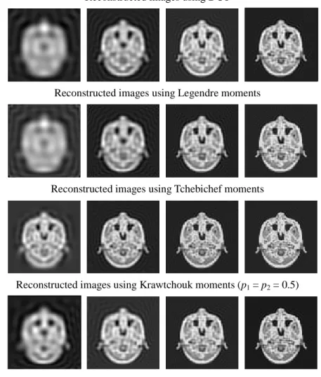
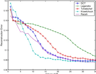
In this example, a magnetic resonance image of size 96 × 96 pixels is used. Fig. 10 shows the reconstruction results for different values of M. Here the parameters are set to a = α = 10, b = 106 and β = 5 for RM and p1 = p2 = 0.5 for
KM. Fig. 11 shows the plot of the mean square errors using different approaches with maximum value of M = 95. The results demonstrate the superiority of Racah moments over the DCT, LM, TM and KM in terms of feature representation capability.
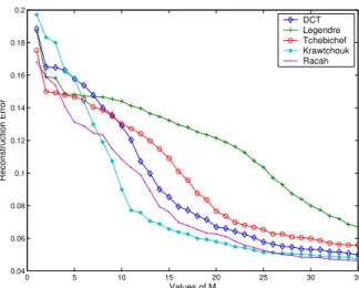
It is well known that the noise may severely affect the image reconstruction quality. To test the robustness of Racah moments with regard to different kind of noises, we apply the proposed moments to some noisy images. We first add the zero mean Gaussian noise with variance 0.2 to a Chinese character of size 40 × 40. Fig. 12 shows the reconstructions using the DCT, LM, TM, KM (p1 = p2 = 0.5), and RM (a = α = 10, b = 50 and β = 5), and the
corresponding error comparison is shown in Fig 13. Note that the reconstruction error is computed with Eq. (49) in which the reconstructed image ~f(s,t) is defined by Eq. (25) for the Racah moments, and by Eq. (53) for the DCT. Fig. 13 indicates that the Krawtchouk moments have the best performance in terms of the noise robustness, and the proposed Racah moments perform better than the DCT and other orthogonal moments.
This analysis is repeated by adding the salt-and-pepper noise (5%) to the same test image. The corresponding results with M = 35 are shown in Figs. 14 and 15. It can be observed from these figures that the proposed method is more robust to noise than the DCT and Legendre and Tchebichef moments. But the Krawtchouk moments (p1 = p2 =
0.5) have the best performance.
As mentioned in Sec. 3.3, when the parameters are set with a = α = β, the permutability property of Racah polynomials about n + a and s can be used to reduce the number of computations of the Racah polynomials by half. Table 1 lists the CPU time of calculating the Racah polynomials for different size images. The computer used in this experiment is a Pentium IV, 2.4GHz, Memory: 1GB.
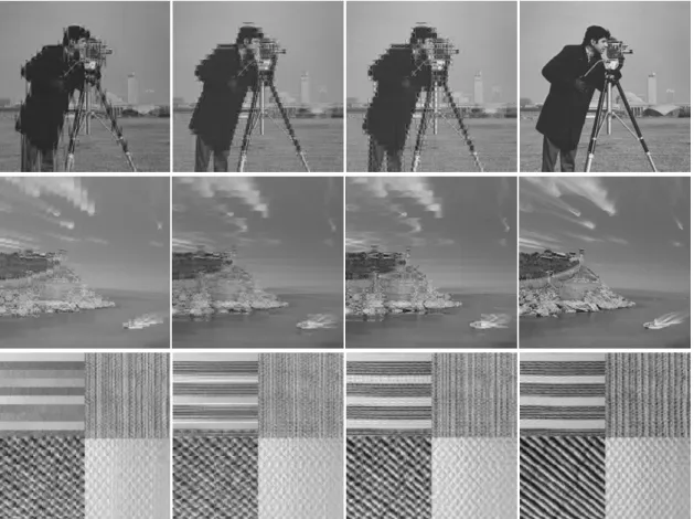
4.2. Image compression
In this subsection, we test the compression capability of the proposed approach, and compare it with other well known transforms. Four test images including “Lena”, “Cameraman”, “Texture” and “Boat” are used in our experiment. Each image is first divided into the sub-blocks whose size is W×W, each block is then transformed by using the DCT, TM, KM, and RM. Fig. 16 shows the basis functions of these four transforms for a block of size 8×8. Since the variance represents the energy or information content of the corresponding transform coefficient, and the transform coefficients with large variances are candidates containing significant features in a pattern-recognition application [29], all the coefficients are rearranged in downward order, and part of them (according to the compression ratio) are chosen to reconstruct the original image. Fig. 17 shows the decoded results of the four test images. In this experiment, the compression ratio is set to 2:1, and the block size is set to 8×8 for “Lena”, “Cameraman”, and “Texture”, and 16×16 for “Boat”. The parameters concerned in KM and RM are chosen as: p1 = p2 = 0.5 for KM and a
= α = 5, β = 0, and b = size of block + a for RM. In order to evaluate the performance of different methods, we use the MSE defined by (49) and the peak signal to noise ratio (PSNR) to quantitatively measure the fidelity of the decoded image. The PSNR of a gray-level image is defined as
10
log
(
255
)
2 10
MSE
PSNR
=
(54) where 255 is the peak image amplitude, and the MSE is defined by (49).Fig. 18 shows the MSE of different methods for the four test images with compression ratio 2:1 and 4:1, respectively. Table 2 lists the corresponding PSNR values. The results indicate that the Racah moments have a better compression capability compared with other transforms.
5. Conclusion
In this paper, we have introduced the Racah polynomials to define a new type of discrete orthogonal moments
known as Racah moments. The Racah polynomials belong to a class of discrete polynomials that are orthogonal on non-uniform lattice. Appropriate scale factors have been used in the moment functions, so that the computed moments are not subject to numerical instability. The properties of the weighted Racah polynomials such as recurrence relations and permutability have been discussed. We have compared the Racah moments with other orthogonal transforms including the DCT, Legendre moments, discrete Tchebichef moments and discrete Krawtchouk moments in terms of the reconstruction capability for images with and without noise. The reconstruction results and detailed error analysis show that the Racah moments perform better than the DCT and Legendre, Tchebichef, and Krawtchouk moments for free-noise images. Conversely, the Krawtchouk moments are more robust to noise. We have also investigated the compression aspect of the proposed Racah moments and compared it with the DCT and other discrete orthogonal moments. The experimental results show a better behavior of the Racah moments in terms of compression capability over the other transforms. The studies show that the proposed moments are potentially useful as feature descriptors for image analysis.
Acknowledgement: This work was supported by National Basic Research Program of China under grant
No.2003CB716102, the National Natural Science Foundation of China under grant No. 60272045, and Program for New Century Excellent Talents in University under grant No. NCET-04-0477. It has been carried out in the frame of the CRIBs, a joint international laboratory associating Southeast University, the University of Rennes 1 and INSERM, with a grant provided by the French Consulate in Shanghai. We thank the anonymous referees for their helpful comments and suggestions.
References
[1] C. W. Chong, P. Raveandran, R. Mukundan, Translation and scale invariants of Legendre moments, Pattern Recognition, 37 (2004) 119-129.
[2] J. H. Yin, A. R. D. Pierro, M. Wei, Analysis for the reconstruction of a noisy signal based on orthogonal moments, Appl. Math. Computat., 132 (2002) 249-263.
[3] N. Kiryati, A. M. Bruckstein, H. Mizrahi, Comments on: Robust line fitting in a noisy image by the method of moments, IEEE Trans. Pattern Anal. Machine Intell., 12 (2000) 1340-1341.
[4]L. M. Luo, X. H. Xie, X. D. Bao, A modified moment-based edge operator for rectangular pixel image, IEEE Trans. Circuits Systems Video Technol., 4 (1994) 552-554.
[5] C. Qing, P. Emil, Y. Xiaoli, A comparative study of Fourier descriptors and Hu's seven moment invariants for image recognition, Canadian Conference on Electrical and Computer Engineering, 1 (2004) 103-106.
[6] M. R. Teague, Image analysis via the general theory of moments, J. Opt. Soc. Amer., 70 (1980) 920-930.
[7] R. Mukundan, S. H. Ong, P. A. Lee, Discrete vs. continuous orthogonal moments for image analysis, International. Conf. on Imaging Science, Systems and Technology-CISST’01 (2001) 23-29.
[8] C. W. Chong, P. Raveendran, R. Mukundan, A comparative analysis of algorithms for fast computation of Zernike moments, Pattern Recognit., 36 (2003) 1765-1773.
[9] H. Z. Shu, L. M. Luo, X. D. Bao, W. X. Yu, An efficient method for computation of Legendre moments, Graphical Models, 63 (2000) 237-262.
[10] R. Mukundan, S. H. Ong, P. A. Lee, Image analysis by Tchebichef moments, IEEE Trans. Image Processing, 10 (2001) 1357-1364.
[11] P. T. Yap, R. Paramesran, S. H. Ong, Image Analysis by Krawtchouk Moments, IEEE Trans Image Processing, 12 (2003) 1367-1377.
[12] M. Lorente, Orthogonal polynomials of several discrete variables and the 3nj-Wigner symbols: applications to spin networks, Math-ph/0402007, (2004) 1- 4.
[13] A. V. Nikiforov, S. K. Suslov, V. B. Uvarov, Classical orthogonal polynomials of a discrete variable. New York: Springer-Verlag, 1991.
[14] R. Alvarez-Nodarse, J. S. Dehesa, Distributions of zeros of discrete and continuous polynomials from their recurrence, Applied Mathematics and Computation, 128 (2002) 167-190.
[15]M. Lorente, Raising and lowening operators factorization and difference operators of hypergeometric type, J.