Final state machine representation of corticogenesis

HAL Id: hal-00553442

https://hal.archives-ouvertes.fr/hal-00553442

HAL is a multi-disciplinary open access archive for the deposit and dissemination of sci-entific research documents, whether they are pub-lished or not. The documents may come from teaching and research institutions in France or abroad, or from public or private research centers.

L’archive ouverte pluridisciplinaire HAL, est destinée au dépôt et à la diffusion de documents scientifiques de niveau recherche, publiés ou non, émanant des établissements d’enseignement et de recherche français ou étrangers, des laboratoires publics ou privés.

Final state machine representation of corticogenesis

Sabina Pfister, Colette Dehay, Henry Kennedy, Rodney Douglas

To cite this version:

Sabina Pfister, Colette Dehay, Henry Kennedy, Rodney Douglas. Final state machine representa-tion of corticogenesis. Cinquième conférence plénière française de Neurosciences Computarepresenta-tionnelles, ”Neurocomp’10”, Aug 2010, Lyon, France. �hal-00553442�

CELL LINEAGE PROJECTIONS IN LOW DIMENSIONAL SPACES

Sabina Pfister*, Colette Dehay**, Henry Kennedy**, Rodney Douglas*

*Institute of Neuroinformatics, UNI/ETH, Zürich, Switzerland **Stem-cell and Brain Research Institute, INSERM, Lyon, France

Corresponding Author: Sabina Pfister, sabina@ini.phys.ethz.ch

ABSTRACT

Cortical neurogenesis is a complex process during which dividing cells have the ability to acquire specific fates and eventually differentiate toward a terminal cell type. The adoption of a cell phenotype is the result of intrinsic programs, which regulate cell behaviour and cell-cell interations. Insight into the mechanisms underlying corticogenesis is provided by the genealogical history of every precursor (cell lineage). We present a method to identify recurrent developmental patterns in lineage trees, where the leaves of the tree are labeled according to the terminal cell fates. We exploit the information contained in the underlying graph structure to classify the progenitors into different subpopulations by means of spectral clustering. We test the method on artifically generated lineage datasets and show that the result constitutes a compact probabilistic state machine description of the developmental process. This approach will enables us to estimate cell states sequences and a developmental distance between the precursors in reconstructed cortical lineages.

KEY WORDS

Cell lineages, spectral clustering, final state machine, cortical development, neurogenesis, genetic networks.

1. Introduction

The mammalian neocortex is an exquisitely organized six-layered structure containing different neuronal cell types and a diverse range of glia cells [1]. During corticogenesis two germinal compartments lining the lateral ventricle, the ventricular zone (VZ) and the subventricular zone (SVZ), generate pyramidal neurons as well as a fraction of the inhibitory neurons.

In the rodent a heterogenous population of precursor cells have been identified. The first progenitor type are neuroepithelial cells (NECs), which produce preplate neurons and after the onset of neurogenesis give raise to radial glial cells (RGPs) [2]. RGPs divide at the apical surface and can differentiate into neurons as well as into intermediate neuronal progenitors (INPs), also known as basal progenitors [3,4,5,6]. RGPs are mainly responsible

for the amplification of the pool of precursors by symmetric cell division as well as generating directly infragranular layers (VI,V) by asymmetric neurogenic divisions. INPs are classified in two distinct classes: INPs in the VZ have short radial morphology and contribute to all cortical layers, whereas IPNs in the SVZ are multipolar and are though to be largely responsible for the generation of granular and supragranular layers (IV, III-II) [7].

During cortical development dividing cells undergo sequential fate restriction, that is a restriction in the types of differrentiated cells produced. The ordered sequence of cell divisions that leads to defined terminal cell fates is controlled by transcriptional networks, epigenetic regulation and cell-cell interactions. Although we may conceivably consider each cell and every cell division as unique, it is reasonable to assume that transitions between similar cell states are the consequence of a common molecular mechanism. Under this assumption stable profiles of gene expression represents defined attractors and can be interpreted as distinct cell fates [8,9].

Despite the numerous studies on cellular processes regulating corticogenesis, there is still poor under-standing of how molecular mechanisms that control cell fate specification are linked to the final cortical cytoarchitecture. What is the logic behind the generation of different neuronal subtypes? And can we describe it in the form of a compact set of rules, a list of state transitions and actions that each cell can undertake locally?

In order to address these questions, we have chosen to investigate the detailed sequence of cell fate specifications, which is provided by the genealogical history of individual precursors. The cell lineage describes the developmental trajectory in the form of a binary tree: the root is the initial precursor cell; the terminal nodes are cells that have reached a terminal phenotype; and the tree topology represents the relationship between all cells that existed at given time point during development. By analyzing the structure of lineage trees, and especially recurring patterns of cell division and differentiation, we wish to identify the major differentiation pathways that lead to different types of pyramidal neurons.

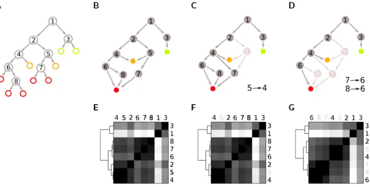
Figure 1. Example of cell division pattern analysis on a small sublineage. We illustrate the cell division pattern analysis

on a small sublineage by showing the state transition diagrams (top row), and the corresponding distance matrices (bottom row). The state transition diagram shows how the cell states are connected to each other, whereas the distance matrix encodes the computed similarity between every cell state pair (black represents complete similarity and white complete dissimilarity). The dendrogram on the left of the matrix indicates the binary linkage between state pairs. (A) Example of an artificially created sublineage starting from a single progenitor #1. Progenitors (gray circles) give rise to 9 terminally differentiated cells (cell type I, light green circles; cell type II, orange circles, cell type III, red circles). Arrows indicate cell division. (B, E) 8-dimensional state transition diagram, which completely describes the sublineage. Arrows indicate the transition probability from one state to the other at cell division. (C, F) 7-dimensional state transition diagram: progenitors #4 and #5 give rise to similar daughter cells and represent a single division mechanism (rule). Redundant part of the lineage are removed from the diagram (light gray circles). (D, G) 5-dimensional state transition diagram: similar division patterns at #7 and #8 can be further reduced to a single rule.

An algorithm that analyzes patterns has been already proposed in the past as an approach to quantify the complexity of metazoan lineages [10]. Inspired by the simple idea that lineages can be expressed as a sequence of division rules, we define a distance measure between cell states in the Euclidean space such that cells with similar progeny are very close to each other. Given experimentally reconstructed genealogical trees in which only terminal cells are labeled according to their phenotype, we can classify the progenitors into different subpopulations.

In the present work we (1) describe the modeling formalism that we use to describe developmental sequences; (2) introduce a method based on spectral clustering theory to perform classification on lineage trees, and (3) validate the method on artificially generated lineage datasets, for which the underlying generative model is known. We propose that developmental programs can be represented with probabilistic finite state machines, a model that describes the rules regulating local cell behavior. We will use the proposed method to analyze reconstructed cell lineages from different areas of the cerebral cortex in the mouse.

2. Results

2.1 State machine description of cell lineages

The generation of different cell subpopulations during cortical development is the result of concurring complex processes, wich involves a variaty of different possible cell states and transitions between those states. As long as we don't have any information about the relationships between differen cell states, any prediction about the generative process would not be better than random guessing. As soon as we can establish relationships between states, we can use this information to estimate their degree of similarity.

This information is provided by the lineage trees arising from every precursor. The lineage contains a wealth of information about the correlation between different cells, their function and anatomical position. The lineage description defines the reachable states (cell types) in which a cell can be found in, and the possibility of transition between states. It can be seen as a series of unique rules, each corresponding to a cell division:

which means: "cell X divides into cells Y and Z with probability P". X is an undifferentiated cell, and Y and Z may be undifferentiated and/or terminal cells of a particular terminal fate. The list of rules provides a complete description of the cell division patters and cell fate specification of the lineage.

We describe progenitor cell behaviour in a compact fashion using probabilistic finite state machines, a model composed of a finite set of states and transition probabilities between those states. Stable or metastable profiles of gene expression are defined as states, and state transitions occurs at the moment of cell division, when a cell has a defined probability to either divide symmetrically or asymmetrically into two daugther cells. To each state transition we associate one or multiple actions. For instance the transition toward a differentiated cell type may induce the activation of the cell migration machinery. The list of state transition and actions constitutes a set of local rules contained in each cell, like an abstract genetic code. For instance, the sublineage in Figure 1A can be completly described by the state diagram in Figure 1B. Nodes of the graph represent all possible cell states and edges represent the transition probabilities at cell division.

2.2 Dimensionalty reduction of state machine models

If we assume every cell and every cell division as unique, we would require a genetic or environmental specification for every single cells produced. This is unlikely given the cost that a huge genome would impose. Indeed it is common to find division rules that are repetitively used in different part of the lineage. Given a graph composed of a set of labeled (terminal differantiated cells) and unlabeled data (progenitor cells), we want to cluster the remaining unlabeled vertices by exploting the global structure of the graph.

In the absence of labeled instances, the problem reduces to spectral clustering on graphs. Spectral graph theory is used to characterize the structural properties of undirected graphs using information conveyed by the eigenvalues and eigenvectors of the Laplacian pseudoinverse [11,12]. The model exploits the graph connectivity to compute a euclidean dissimilarity measure called average commute time N. The average commute time is a measure of the connectivity strength between node pairs and has the interesting property of decreasing when the number of paths connecting two nodes increases and when the length of any path decreases.

Conventional spectral clustering does not take into account the presence of labeled nodes in the graph. In order to incorporate information from the labeled instances, we exclusively consider distances from unlabeled nodes r to labeled nodes s and recompute the distance matrix on this values only. Every progenitor cell is thus defined by the distances to all the terminal cell fates that it can generate, and we call this measure developmental distance:

VG is the volume of the graph and xi is the coordinate

vector of the embedding of node i into the Euclidean space. xi are exactly separated by the average commute

time distance to labeled nodes.

The developmental distance is a measure of the similarity between cell states based on shared progeny and ancestors. It captures both genetic and spatial closeness in the lineage. Precursors that generate similar distribution of cells are very closed from each other (genetic closeness), but precursor that share common ancestors are also likely to be closed to each other (spatial closeness). These nice property is a direct consequence of the fact that we use the average commute time rather than the hitting time to compute similarities. Cell states are clustered based on the developmental distance by means of hierarchical clustering with the single linkage algorthim. An example of spectral embedding of a small sublineage in different dimensions is provided in Figure 1. State diagrams (top row) and dissimilarity matrix (bottom row) for the 8, 7 and 5 dimensional models are illustrated. The dissimilarity matrix encodes the degree of similarity between precursors in term of the terminal cell fates of their progeny. When the distance between two states is close to zero or less than a certain treshold, they can be merged into a single state (or division rule).

The model dimension can be choosen by setting the number of different clusters or directly by selecting a particular treshold. The correct parameter is obtained by maximising the dimensionality reduction while preserving the original distribution of terminal cells. This is due to the balance between information compression and information loss. By successively combining nodes we obtain a set of reduced rules encoding a unique description of a lineage set in the form of a probabilistic final state machine. The reduced rules represent core sublineages that can be organized into developmental modules.

2.3 Model recovery in artificial lineage datasets

Can we use the spectral clustering method to discover hidden generative models in lineage datasets? To answer this question we test the alghoritm on artificially generated lineage trees. We select random probabilistic finite state machines models and generates up to 30 lineages for model. The task is to recover the original model from the information provided by the generated lineages.

Despite the presence of noise in the cell division patterns, the clustering algorithm correctly classifies in average between 80-90% of the precursor cells. Depending on the noise levels or the model complexity, the spectral clustering performs slightly differently.

From the classification we can compute the transition probabilities between states and thus generate a final state machine representation of developmental programs.

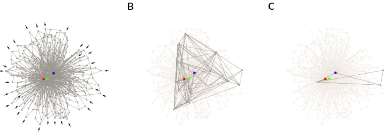
Figure 2. Recovering of hidden state machine model from an artificially generated lineage dataset. Recurring pattern

of cell division and differentiation in artificial lineage datasets are identified by means of spectral clustering analysis. As an example we show a pool of 30 lineages generated with a probabilistic generative model selected at random. We illustrate the data by showing the state transition diagram with (A) 501, (B) 18 and (C) 3 dimensions, when most of the nodes have been merged and discarded from the state diagram (light gray circles). The state transition diagram shows how the cell states are connected to each other, as described in Figure 1 for a simpler example. The original generative model has been correcctly extrapolated and corresponds to case C. The color code of terminally differentiated cell types is: progenitor, dark gray; cell type I, blue circle; cell type II, green circle, cell type III, red circle. Black arrows indicates the position of all the 30 initial progenitors.

3. Discussion

The key to understand the complexity of mature cerebral cortex architecture, both in mouse and in the primate, resides in the developmental process. The patterns of intra- and interareal connectivity are a direct consequence of the number, specificity, timing and position of the neurons generated and the connectivity itself is used to shape the functional structure of the cortex [13]. An interesting question is how the regulatory system, a network composed of more than thousand of genes, determins cell fate diversity and leads to a defined cytoarchitecture.

One way to adress this question would be a systematic analysis of in vivo gene expression profiles of dividing cells during the whole corticogenesis, which is notably difficult to obtain were a huge number of cells is involved, such as in the mouse and monkey cerebral cortex. We propose a strategy to infer this kind of information from a reduced dataset, which would be more easy retrieved experimentally. The proposed method has the advantage that requires only semi-labeled data (cell lineage in which only the terminal cell fates are labeled) and could be applied to any recorded database of cell division patterns. Obviously the quality of the classification strongly depends on the labels of the differentiated cells. A more precise distinction between terminal fates means a finer classification. The model can be refined as more different terminal fates are discovered. We have analyzed artificially generated datasets of cell lineages (for which the generative model is known) and

showed that the underlying model can be sucessfully recovered using spectral clustering. The alghoritm selects a list of states and state transitions that can be recursively used to specify the sequences of developmental events. A similiar approach used to quantify lineage complexity as already been proposed [10]. In contrast to previous work, we don't restrict ourselfs to a deterministic model, but rather use probabilistic final state machines to describe developmentl programs. The advantage is the ability to recover recurring motives even in the presence of noise or stochastic processes since we cluster cell states based on a similarity measure and not on exact matches of graph connectivities. Moreover the developmental distance takes into account spatial distance (cells that are born in spatial proximity are assumed to share the same environment and thus are more likely to have the same behaviour). Although not implemented yet into the model, finite state machines are also able to read input from the environment and be influenced accordingly.

It should be noted that in our approach the model is not a set of differential equations that can be numerically solved, but rather a computational model, a state machine relating different cellular configurations to each other. Computational models have the advantage of being qualitative and thus particularly useful to test hypothesis without the need of huge parametric searches, as is the case of conventional genetically inspired algorithms. We will apply the described reconstruction of finite state machine diagram to cortical lineages from different cortical areas and from different experimental conditions.

4. Methods

4.1 Spectral clustering

We use a spectral clustering method [11,12] to efficiently identify recurring motives in the lineage tree. Spectral graph theory is used to characterize the structural properties of undirected graphs using information conveyed by the eigenvalues and eigenvectors of the Laplacian pseudoinverse. The method exploits the graph structure to compute a dissimilarity measure between nodes of the graph.

Briefly, we consider a weighted undirected graph G with symmetric weights wij and n nodes. The elements aij of

the adjacency matrix A are defined as aij = wij if node i is

connected to node j and 0 otherwise. The Laplacian matrix L of the graph is defined by L = D−A, where D is the degree matrix and VG is the volume of the graph.

The average commute time N is defined as the average number of steps a random walker, starting from node i will take before entering node j for the first time, and go back to i. This distance measure has the interesting property of decreasing when the number of paths connecting the two nodes increases and when the length of any path decreases.

We compute the commute time from the Moore-Penrose pseudoinverse of the Laplacian matrix L+ _{as following:}

where each node i is represented by a unit vector ei in the

Euclidean space Rn _{since L}+ _{is positive semidefinite.}

The spectral decomposition of L+ _{is defined as L}+_=UΛUT_,

where Λ is the diagonal matrix with the ordered eigenvalues as elements, and U is the ordered orthonormal matrix with eigenvectors of L+ _{as columns.}

Based on the eigenvector decomposition of L+_{, the nodes}

vectors ei can be mapped into a new Euclidean space that

preserves the commute time distance. Furthermore the spectral decomposition projects the node vectors on the principal components so that L+ can be approximated by considering only the m < (n− 1) first eigenvectors.

with:

Since the projection in x preserves the commute time, the Euclidean distance between the nodes can be interpreted as a similarity measure. In order to analyze information from the labeled instances, we exclusively consider distances from unlabeled nodes r to labeled nodes s and recompute the distance matrix on this values only. The new distance measure is defined by:

Binary clustering on the new distance measure is computed by the single linkage algorithm.

Data analysis and data visualization were performed using Matlab and the statistical open source software R.

References

[1] Molyneaux, B. J., Arlotta, P., Menezes, J. R. L., and Macklis, J. D., Nat Rev Neuro 8(6), 2007, 427–437. [2] Götz, M. & Huttner, W., Nat Rev Mol Cell Biol 6(10), 2005, 777–788.

[3] Haubensak, W., Attardo, A., Denk, W. & Huttner, W. B., PNAS 101, 2004, 3196-3201.

[4] Miyata, T. et al., Development 131(13), 2004, 3133-3145.

[5] Noctor, S. C., Martnez-Cerde~no, V., Ivic, L. & Kriegstein, A. R., Nature neuroscience 7(2), 2004, 136-144.

[6] Attardo, A., Calegari, F., Haubensak, W., Wilsch-Bräuninger, M. & Huttner, W. B., PLoS ONE 3(6), 2008, e2388.

[8] Kauman, S., The origins of order: self-organization

and selection in evolution (Oxford University Press,

1993).

[9] Huang, S., Eichler, G., Bar-Yam, Y. & Ingber, D.,

Physical review letters 94(12), 2005, 128701.

[10] Azevedo, R. et al., Nature 433(7022), 2005, 152156. [11] Qiu, H. & Hancock, E., IEEE Transactions on

Pattern Analysis and Machine Intelligence 29(11), 2007,

1873.

[12] Fouss, F., Pirotte, A., Renders, J.-M. & Saerens, M.,

IEEE Transactions on Knowledge and Data Engineering 19(3), 2007, 355-369.

[13] Dehay, C. & Kennedy, H., Nature Reviews