HAL Id: hal-02126848
https://hal.archives-ouvertes.fr/hal-02126848
Submitted on 15 May 2019
HAL is a multi-disciplinary open access
archive for the deposit and dissemination of
sci-entific research documents, whether they are
pub-lished or not. The documents may come from
teaching and research institutions in France or
abroad, or from public or private research centers.
L’archive ouverte pluridisciplinaire HAL, est
destinée au dépôt et à la diffusion de documents
scientifiques de niveau recherche, publiés ou non,
émanant des établissements d’enseignement et de
recherche français ou étrangers, des laboratoires
publics ou privés.
Comparing systems: max-case refinement orders and
application to differential privacy
Konstantinos Chatzikokolakis, Natasha Fernandes, Catuscia Palamidessi
To cite this version:
Konstantinos Chatzikokolakis, Natasha Fernandes, Catuscia Palamidessi.
Comparing systems:
max-case refinement orders and application to differential privacy.
CSF 2019 - 32nd IEEE
Computer Security Foundations Symposium, Jun 2019, Hoboken, United States.
pp.442–457,
Comparing systems: max-case refinement orders
and application to differential privacy
Konstantinos Chatzikokolakis
University of Athens [email protected]
Natasha Fernandes
INRIA and Ecole Polytechnique [email protected]
Catuscia Palamidessi
INRIA and Ecole Polytechnique [email protected]
Abstract—Quantitative Information Flow (QIF) and Differ-ential Privacy (DP) are both concerned with the protection of sensitive information, but they are rather different approaches. In particular, QIF considers the expected probability of a successful attack, while DP (in both its standard and local versions) is a max-case measure, in the sense that it is compromised by the existence of a possible attack, regardless of its probability. Comparing systems is a fundamental task in these areas: one wishes to guarantee that replacing a system A by a system B is a safe operation, that is the privacy of B is no-worse than that of A. In QIF, a refinement order provides strong such guarantees, while in DP mechanisms are typically compared (wrt privacy) based on the ε privacy parameter that they provide.
In this paper we explore a variety of refinement orders, inspired by the one of QIF, providing precise guarantees for max-case leakage. We study simple structural ways of characterising them, the relation between them, efficient methods for verifying them and their lattice properties. Moreover, we apply these orders in the task of comparing DP mechanisms, raising the question of whether the order based on ε provides strong privacy guarantees. We show that, while it is often the case for mechanisms of the same “family” (geometric, randomised response, etc.), it rarely holds across different families.
I. INTRODUCTION
The enormous growth in the use of internet-connected de-vices and the big-data revolution have created serious privacy concerns, and motivated an intensive area of research aimed at devising methods to protect users’ sensitive information. During the last decade, two main frameworks have emerged in this area: Differential Privacy (DP) and Quantitative Infor-mation Flow (QIF).
Differential privacy (DP) [1] was originally developed in the area of statistical databases, and it aims at protecting the individuals’ data while allowing the release of aggregate infor-mation via a query. This is obtained by obfuscating the query outcome via the addition of controlled noise. More recently, also some distributed variants of DP have been proposed: Local differential privacy (LDP) [2] and d-privacy [3]. They are distributed in the sense that in these models the personal data are obfuscated at the users’ end before they are collected. In this way, there is no need to ensure that the entity collecting and storing the data is honest and capable of protecting the data from security breaches.
This work has been partially supported by the project ANR-16-CE25-0011 REPAS and by the Equipe Associ´ee LOGIS
The definition of d-privacy assumes an underlying metric structure on the data domain X , and, from a mathematical point of view, it can be viewed as an extension of both DP and LDP. To illustrate this point we need to describe the property that expresses d-privacy. An obfuscation mechanism K for X is a probabilistic mapping from X to some output domain Y, namely a function from X to probabilistic distributions over Y. We will use the notation Kx,y to represent the probability
that K on input x gives output y. The mechanism K is ε·d-private, where ε is a parameter representing the privacy level, if
Kx1,y≤ e
ε d(x1,x2)K
x2,y for allx1, x2∈ X , y ∈ Y. (1)
Standard DP is obtained from this definition by assuming X to be a set of all datasets and d the Hamming distance (i.e., the number of records in which two datasets differ)1. LDP is
obtained by considering a trivial metric (distance 0 between identical elements, and 1 otherwise). In this paper we will use d-privacy as a unifying framework.
Research on quantitative information flow (QIF) focuses on the potentialities and the goals of the attacker and it has developed rigorous foundations based on information theory [4], [5]. The idea is that a system processing some sensitive data from a random variable X and releasing some observable data as a random variable Y can be modelled as an information-theoretic channel with input X and output Y . The leakage is then measured in terms of correlation between X and Y . There are, however, many different ways to define such correlation, depending on the notion of adversary. In order to provide a unifying approach, [6] has proposed the theory of g-leakage, in which an adversary is characterized by a functional parameter g representing its gain for each possible outcomes of the attack.
Providing a rigorous way to compare mechanisms from the point of view of their privacy guarantees is a fundamental issue in the design and the implementation of mechanisms for information protection. In this respect, the QIF approach has lead to an elegant theory of refinement (pre)order2 vavgG , which provides strong guarantees: A vavgG B means that B
1The more common definition of differential privacy assumes that x1, x2 are adjacent, i.e. their Hamming distance is 1, and requires Kx1,y ≤
eεKx
2,y. It is easy to prove that the two definitions are equivalent.
2In this paper we call vavg
G and the other refinement relations “orders”, although, strictly speaking they are preorders.
is safer than A in all circumstances, in the sense that the expected gainof an attack on B is less than on A, for whatever kind of gain the attacker may be seeking. This means that we can always substitute the component A by B without compromising the security of the system. An appealing aspect of this particular refinement order is that it is characterized by a precise structural relation between the stochastic channels associated to A and B [6], [7], which makes it easy to reason about, and relatively efficient to verify. It is important to remark that this order is based on an average notion of adversarial gain (vulnerability), defined by mediating over all possible observations and their probabilities. We call this perspective average-case.
At the other end of the spectrum, DP, LDP and d-privacy are max-case measures. In fact, by applying the Bayes theorem to (1) we obtain: p(x1| y) p(x2| y) ≤ eε d(x1,x2)π(x1) π(x2) for allx1, x2∈ X , y ∈ Y. (2) where π(xi) is the prior probability of xi and p(xi| y) is the
posteriorprobability of xigiven y. We can interpretπ(x1)/π(x2)
andp(x1|y)/p(x2|y)as knowledge about X : they represent how
much more likely x1 is with respect to x2, before (prior) and
after (posterior) observing y, respectively. Thus the property expresses a bound on how much the adversary can learn from each individual outcome of the mechanism3.
In the literature of DP, LDP and d-privacy, mechanisms are usually compared on the basis of their ε-value4, which controls a bound on the log-likelihood ratio of an observation y given two “secrets” x1 and x2: smaller ε means more privacy. In
DP and LDP the bound is ε itself, while in d-privacy it is ε × d(s1, s2) We remark that the relation induced by ε in
d-privacy is fragile, in the sense that the definition of d-d-privacy assumes an underlying metric structure d on the data, and whether a mechanism B is “better” than A depends in general on the metric considered.
Average-case and max-case are different principles, suitable for different scenarios: the former represent the point of view of an organization, for instance an insurance company providing coverage for risks related to credit cards, which for the cost-benefit analysis is interested in reasoning in terms of expectation (expected cost of an attack). The max-case represents the point of view of an individual, who is interested in limiting the cost of any attack. As such, the max-case seems particularly suitable for the domain of privacy.
In this paper, we combine the max-case perspective with the robustness of the QIF approach, and we introduce two refinement orders:
• vmax
Q , based on the max-case leakage introduced in [9].
This order takes into account all possible privacy breaches
3The property (2) is also the semantic interpretation of the guarantees of the Pufferfish framework (cfr. [8], Section 3.1). The ratio p(x1|y)p(x2|y)/π(x1)
π(x2) is
known as odds ratio.
4In DP and LDP ε is a parameter that usually appears explicitly in the definition of the mechanism. In d-privacy it is an implicit scaling factor.
caused by any observable (like in the DP world), but it quantifies over all possible quasi-convex vulnerability functions (in the style of the QIF world).
• vprv
M , based on d-privacy (like in the DP world), but
quantified over all metrics d.
To underline the importance of a robust order, let us consider the case of the oblivious mechanisms for differential privacy: These mechanisms are of the form K = H ◦ f , where f : X → Y is a query, namely a function from datasets in X to some answer domain Y, and H is a probabilistic mechanism implementing the noise. The idea is that the system first computes the result y ∈ Y of the query (true answer), and then it applies H to y to obtain a reported answer z. In general, if we want K to be ε-DP, we need to tune the mechanism H so to take into account the sensitivity of f , which is the maximum distance between the results of f on two adjacent databases, and as such it depends on the metric on Y. However, if we know that K = H ◦ f is ε-DP, and that H vprv
M H
0 for some other mechanism H0, then we can
safely substitute H by H0 as it is, because one of our results (cfr. Theorem 6 at Page 7) guarantees that K0 = H0 ◦ f is also ε-DP. In other words, H vprvM H0 implies that we can substitute H by H0 in an oblivious mechanism for whatever query f and whatever metric on Y, without the need to know the sensitivity of f and without the need to do any tuning of H0 . Thanks to Theorem3(Page6) and Theorem5 (Page7),
we know that this is the case also for vavgG and vmaxQ . As an example, consider datasets x ∈ X of records containing the age of people, expressed as natural numbers from 0 to 100, and assume that each dataset in X contains at least 100 records. Consider two queries, f (x) and g(x), which give the rounded average age and the minimum age of the people in x, respectively. Finally, consider the truncated geometric mechanism T Gε (cfr. Definition 10, Page 9), and the randomized response mechanism Rε (cfr. Definition 13, Page 10). It is easy to see that K1 = T Gε◦ f is ε-DP, and
it is possible to prove that T Gε vprv M R
ε (cfr. Theorem 16,
Page 16). We can then conclude that K2 = Rε◦ f is ε-DP
as well, and that in general it is safe to replace T Gε by Rε
for whatever query. On the other hand, Rε 6vprv M T G
ε, so
we cannot expect that it is safe to replace Rεby T Gεin any
context. In fact, K3= Rε◦ g is ε-DP, but K4= T Gε◦ g is not
ε-DP, despite the fact that both mechanisms are constructed using the same privacy parameter ε. Hence we can conclude that a refinement relation based only on the comparison of the ε parameters would not be robust, at least not for a direct replacement in an arbitrary context. Note that K4is 100 ×
ε-DP. In order to make it ε-DP we should divide the parameter ε by the sensitivity of g (with respect to the ordinary distance on natural numbers), which is 100, i.e. use T Gε/100. For Rε
this is not necessary because it is defined using the discrete metric on {0, . . . , 100}, and the sensitivity of g with respect to this metric is 1.
The robust orders allow us to take into account different kinds of adversaries. Consider for instance the following three LDP mechanisms, represented by their stochastic matrices
(where each element is the conditional probability of the outcome of the mechanism, given the secret value). The secrets are three possible economic situations of an individual, p, a and r, standing for poor, average and rich, respectively. The observable outcomes are r and n, standing for rich and not rich. A n r p 3/4 1/4 a 1/2 1/2 r 1/4 3/4 B n r p 2/3 1/3 a 2/3 1/3 r 1/3 2/3 C n r p 2/3 1/3 a 1/2 1/2 r 1/3 2/3
Let us assume that the prior distribution π on the secrets is uniform. We note that A is (log 3)-LDP while B is (log 2)-LDP. Hence, if we only look at the value of ε, we would think that B is better than A from the privacy point of view. However, there are attackers that gain more from B than from A (which means that, with respect to those attackers, the privacy of B is worse). For instance, this is the case when the attacker is only interested in discovering whether the person is rich or not. In fact, if we consider a gain 1 when the attacker guesses the right class (r versus (either p or a)) and 0 otherwise, we have that the highest possible gain in A is (3/4) π(p) + (1/2) π(a) = 5/12, while in B is
(2/3) π(p) + (2/3) π(a) =4/9, which is higher than 5/12. This
is consistent with our orders: it is possible to show that none of the three orders hold between A and B, and that therefore we should not expect B to be better (for privacy) than A with respect to all possible adversaries.
On the other hand, the mechanism C is also (log 2)-LDP, and in this case we have that the relation A vmax
Q C holds,
implying that we can safely replace A by C. We can also prove that the reverse does not hold, which means that C is strictly better than A.
A fundamental issue is how to prove that these robust orders hold: Since vmaxQ and vprvM involve universal quantifications, it is important to devise finitary methods to verify them. To this purpose, we will study their characterizations as structural relations between stochastic matrices (representing the mechanisms to be compared), along the lines of what was done for vavgG .
We will also study the relation between the three orders (the two above and vavg
G ), and their algebraic properties.
Finally, we will analyze various mechanisms for DP, LDP, and d-privacy to see in which cases the order induced by ε is consistent with the three orders above.
A. Contribution
The main contributions of this paper are the following:
• We introduce two refinement orders for the max case, vmax
Q and v
prv
M , that are robust with respect to a large
class of adversaries.
• We give structural characterizations of both vmaxQ and vprvM in terms of relations on the stochastic matrices of the mechanisms under comparison. These relations help the intuition and open the way to verification.
• We study efficient methods to verify the structural
rela-tions above. Furthermore, these methods are such that, when the verification fails, they produce counterexam-ples. In this way it is possible to pin down what is the problem and try to correct it.
• We show that vavg ⊂ vmax ⊂ vprv.
• We apply the three orders (vavgG , vmaxQ , and vprvM ) to the comparison of some well-known families of d-private mechanisms: geometric, exponential and randomised re-sponse. We show that, in general, A vavgG B (and thus all the refinement orders between A and B) holds within the same family whenever the ε of B is smaller than that of A.
• We show that if A and B are mechanisms from different
families, then, even if the ε of B is smaller than that of A, the relations A vavgG B and A vmax
Q B do not hold,
and in most cases A vprv
M B does not hold either. We
conclude that a comparison based only on the value of the ε’s is not robust across different families, at least not for the purposes illustrated above.
• We study lattice-properties of these orders. In contrast to vavgG , which was shown to not be a lattice, we prove that suprema and infima exist for vmaxQ and vprvM , and that therefore these orders form lattices.
B. Related work
We are not aware of many studies on refinement relations for QIF. Yasuoka and Terauchi [10] and Malacaria [11] have explored strong orders on deterministic mechanisms, focusing on the fact that such mechanisms induce partitions on the space of secrets. They showed that the orders produced by min-entropy leakage [5] and Shannon leakage [12], [13] are the same and, moreover, they coincide with the partition refinement order in the Lattice of Information [14]. This order was extended to the probabilistic case in [6], resulting in the relation vavg mentioned in Section II. The same
paper [6] proposed the theory of g-leakage and introduced the corresponding order vavg
G . Furthermore, [6] proved that
vavg⊆ vavg
G and conjectured that also the reverse should hold.
This conjecture was then proved valid in [7]. The max-case leakage, on which the relation vmax
Q is based, was introduced
in [9], but vmaxQ and its properties were not investigated. Finally, vprv is a novel notion introduced in this paper.
In the field of differential privacy, on the other hand, there have been various works aimed at trying understand the operational meaning of the privacy parameter ε and at providing guidelines for the choice of its values. We mention for example [15] and [16], which consider the value of ε from an economical point of view, in terms of cost. We are not aware, however, of studies aimed at establishing orders between the level of privacy of different mechanisms, except the one based on the comparison of the ε’s.
The relation between QIF and DP, LDP, and d-privacy is based on the so-called semantic interpretation of the privacy notions, that regards these properties as expressing a bounds on the increase of knowledge (from prior to posterior) due
to the answer reported by the mechanism. For d-privacy the semantic interpretation is expressed by (2). To the best of our knowledge, this interpretation was first pointed out (for the location privacy instance) in [17]. The seminal paper on d-privacy, [3], also proposed a semantic interpretation, with a rather different flavor, although formally equivalent. As for DP, as explained in the introduction, (2) instantiated to databases and Hamming distance corresponds to the odds ratio on which is based the semantics interpretation provided in [8]. Before that, another version of semantic interpretation was presented in [1] and proved equivalent to a form of DP called ε-indistinguishability. Essentially, in this version an adversary that queries the database, and knows all the database except one record, cannot infer too much about this record from the answer to the query reported by the mechanism. Later on, an analogous version of semantic interpretation was reformulated in [18] and proved equivalent to DP. A different interpretation of DP, called semantic privacy, was proposed by [19]. This interpretation is based on a comparison between two posteriors (rather between the posterior and the prior), and the authors show that, within certain limits, it is equivalent to DP. C. Plan of the paper
In the next three sections, II, III and IV, we define the order refinements vavg
G , v max
Q and v
prv
M respectively, and we
study their properties. In SectionV-Awe investigate methods to verify them. In SectionVIwe consider various mechanisms for DP and its variants, and we investigate the relation between the parameter ε and the orders introduced in this paper. In Section VII we show that vmaxQ and vprvM form a lattice. Finally, Section VIIIconcludes.
II. AVERAGE-CASE REFINEMENT
A. Vulnerability, channels and leakage
Quantitative Information Flow studies the problem of quan-tifying the information leakage of a system (eg. a program, or an anonymity protocol). A common model in this area is to consider that the user has a secret x from a finite set of possible secrets X , about which the adversary has some probabilistic knowledge π: DX (DX denoting the set of probability distributions over X ). A function V : DX → R≥0
is then employed to measure the vulnerability of our system: V (π) quantifies the adversary’s success in achieving some desired goal, when his knowledge about the secret is π.
Various such functions can be defined (eg. employing well-known notions of entropy), but it quickly becomes apparent that no single vulnerability function is meaningful for all systems. The family of g-vulnerabilities [6] tries to address this issue by parametrizing V in an operational scenario: first, the adversary is assumed to possess a set of actions W; second, a gain function g(w, x) models the adversary’s gain when choosing action w and the real secret is x. g-vulnerability can be then defined as the expected gain of an optimal guess: Vg(π) = maxw: WPx: Xπxg(w, x). Different adversaries can
be modelled by proper choices of W and g. We denote by GX the set of all gain functions.
Defn Vulnerabilities SectionII-A V [π, C] := P
yayV (δy) SectionIII Vmax[π, C] := maxyV (δy)
Definition8 Vd(π) := inf{ε ≥ 0 | ∀x, x0∈ X , πx≤ eε·d(x,x0)π x0}
Defn Leakage Measures
Definition4 Privd(C) := inf{ε ≥ 0 | C satisfies ε · d-privacy} Equation (4) L+,maxd (π, C) := Vmax
d [π, C] − Vd(π) Equation (5) ML+,maxd (C) := maxπL+,maxd (π, C)
Defn Refinement Orders
SectionII-B A vavgB iff AR = B for some channel R Definition2 A vmaxB iff R ˜A = ˜B for some channel R Definition7 A vprvB iff B satisfies dA-privacy
Defn Leakage Orders SectionII-B A vavg
G B iff ∀g: GX , ∀π: DX , Vg[π, A] ≥ Vg[π, B] Definition1 A vmax Q B iff ∀V : QX , ∀π: DX , V max[π, A] ≥ Vmax[π, B] Definition6 A vprv M B iff ∀d ∈ MX , A v prv d B Definition5 A vprvd B iff Privd(A) ≥ Privd(B)
TABLE I
DEFINITIONS AND SYMBOLS USED IN THIS PAPER.
A system is then modelled as a channel: a probabilistic mapping from the (finite) set of secrets X to a finite set of observations Y, described by a stochastic matrix C, where Cx,y is the probability that secret x produces the observation
y. When the adversary observes y, he can transform his initial knowledge π into a posterior knowledge δy
: DX . Since each observation y is produced with some probability ay, it is
sometimes conceptually useful to consider that the result of running a channelC, on the initial knowledge π, is a “hyper” distribution [π, C]: a probability distribution on posteriors δy, each having probability ay.
It is then natural to define the (average-case) posterior vulnerability of the system by applying V to each posterior δy, then averaging by its probability a
y of being produced:
V [π, C] := P
yayV (δy) .
When defining vulnerability in this way, it can be shown [9] that V has to be convex on π, otherwise fundamental properties (such as the data processing inequality) are violated. Any continuous and convex function V can be written as Vg for a
properly chosen g, so when studying average-case leakage we can safely restrict to using g-vulnerability.
Leakagecan be finally defined by comparing the prior and posterior vulnerabilities, eg. as L+g(π, C) = Vg[π, C]−Vg(π).5
5Comparing vulnerabilities “multiplicatively” is also possible, but is or-thogonal to the goals of this paper.
B. Refinement
A fundamental question arises in the study of leakage: can we guarantee that a system B is no less safe than a system A? Having a family of vulnerability functions, we can naturally define a strong order vavgG on channels by explicitly requiring that B leaks6 no more than A, for all priors π and all gain
functions g: GX :7
A vavg
G B iff Vg[π, A] ≥ Vg[π, B]
for all g: GX , π: DX . Although vavg
G is intuitive and provides clear leakage
guar-antees, the explicit quantification over vulnerability functions makes it hard to reason about and verify. Thankfully, this order can be characterized in a “structural” way, that is as a direct property of the channel matrix. We first define the refinement order vavg on channels by requiring that B can be obtained by post-processing A by some other channel R, that is:
A vavgB iff AR = B for some channel R . A fundamental result [6], [7] states that vavg and vavg
G
coincide.
We read A vavg B as “A is refined by B”, or “B is as safe as A”. When A vavg B holds we have a strong privacy guarantee: we can safely replace A by B without decreasing the privacy of the system, independently from the adversary’s goals and his knowledge. But refinement can be also useful in case A 6vavg B; namely, we can conclude that there must exist some adversary, modelled by a gain function g, and some initial knowledge π, such that the adversary actually prefers to interact with A rather than interacting with B.8Moreover, we
can actually construct such a “counter-example” gain function; this is discussed in §V.
III. MAX-CASE REFINEMENT
Although vavg, vavgG provide a strong and precise way of comparing systems, one could argue that average-case vulnerability might underestimate the threat of a system. More precisely, imagine that there is a certain observation y such that the corresponding posterior δy is highly vulnerable (eg. the adversary can completely infer the real secret), but y happens with very small probability ay. In this case the
average-case posterior vulnerability V [π, C] can be relatively small, although V (δy) is large for that particular y.
If such a scenario is considered problematic, we can natu-rally quantify leakage using a max-case9 variant of posterior
vulnerability, where all observations are treated equally regard-less of their probability of being produced:
Vmax[π, C] := max
yV (δy) .
6Note that comparing the leakage of A, B is equivalent to comparing their posterior vulnerability, so we choose the latter for simplicity.
7
Note also that quantifying over g: GX is equivalent to quantifying over all continuous and convex vulnerabilities.
8Whether this adversary is of practical interest or not is a different issue, but we know that there exists one.
9Also called “worse”-case in some contexts, although the latter is more ambiguous, “worse” can refer to a variety of factors.
Under this definition, it can be shown [9] that V has to be quasi-convex on π (instead of convex), in order to satisfy fundamental properties (such as the data processing inequal-ity). Hence, in the max-case, we no longer restrict to g-vulnerabilities (which are always convex), but we can use any vulnerability V : QX , where QX denotes the set of all continuous quasi-convex functions DX → R≥0.
Inspired by vavgG , we can now define a corresponding max-case leakage order.
Definition 1. The max-case leakage order is defined as A vmaxQ B iff Vmax[π, A] ≥ Vmax[π, B]
for allV : QX , π: DX . Similarly to its average-case variant, vmax
Q provides clear
privacy guarantees by explicitly requiring that B leaks no more than A for all adversaries (modelled as a vulnerability V ). But this explicit quantification make the order hard to reason about and verify. We would thus like to characterize vmaxQ by a refinement order that depends only on the structure of the two channels.
Given a channel C from X to Y, we denote by ˜C the channel obtained by normalizing10 C’s columns and then transposing: ˜ Cy,x := Cx,y P xCx,y .
Note that the row y of ˜C can be seen as the posterior distribution δy obtained by C under the uniform prior. Note
also that ˜C is non-negative and its rows sum up to 1, so it is a valid channel from Y to X . The average-case refinement order required that B can be obtained by post-processing A. We define the max-case refinement order by requiring that ˜B can be obtained by pre-processing ˜A.
Definition 2. The max-case refinement order is defined as A vmaxB iff R ˜A = ˜B for some channel R.
Our goal now is to show that vmaxQ and vmaxare different characterizations of the same order. To do so, we start by giv-ing a “semantic” characterization of vmax, that is, expressing it, not in terms of the channel matrices A and B, but in terms of the posterior distributions that they produce. Thinking of [π, C] as a (“hyper”) distribution on the posteriors produced by π and C, its support supp [π, C] is the set of all posteriors produced with non-zero probability. We also denote by ch S the convex hull of S.
Theorem 1. Let π: DX . If A vmax B then the posteriors of B (under π) are convex-combinations of those of A, that is
supp [π, B] ⊆ ch supp [π, A] . (3) Moreover, if (3) holds and π is full support then A vmaxB.
Note that if (3) holds for any full-support prior, then it must hold for all priors.
We are now ready to give the main result of this section.
Theorem 2. The orders vmax and vmax
Q coincide.
Similarly to the average case, A vmaxB gives us a strong leakage guarantee: can safely replace A by B, knowing that for any adversary, the max-case leakage of B can be no-larger than that of A. Moreover, in case A 6vmaxB, we can always
find an adversary, modelled by a vulnerability function V , who prefers (wrt the max-case) interacting with A that with B. Such a function is discussed in §V.
Finally, we resolve the question of how vmaxand vavgare
related.
Theorem 3. vavg is strictly stronger thanvmax.
This result might appear counter-intuitive at first; one might expect A vmax B to imply A vavg B. To understand why it does not, note that the former only requires that, for each output yB of B, there exists some output of yA that is at
least as vulnerable, regardless of how likely yA and yB are to
happen (this is max-case, after all). Consider, for instance, the following example: A y1 y2 y3 y4 x1 3/4 0 1/4 0 x2 3/4 1/4 0 0 x3 0 1/4 1/4 1/2 B y1 y2 y3 x1 1/2 0 1/2 x2 1/2 1/2 0 x3 0 1/2 1/2 .
Under the uniform prior, the y1, y2, y3 posteriors for both
channels are the same, namely (1/2,1/2, 0), (0,1/2,1/2) and
(1/2, 0,1/2) respectively. So the knowledge that can be obtained
by each output of B can be also obtained by some output of A (albeit with a different probability). Hence, from Thm.1we get that A vmax B. However, we can check (see §V-A) that B cannot be obtained by post-processing A, that is A 6vavgB.
The other direction might also appear tricky: if B leaks no more than A in the average-case, it must also leak no more than B in the max-case. The quantification over all gain functions in the average-case is powerful enough to “detect” differences in max-case leakage. The above result also means that vavg could be useful even if we are interested in the max-case, since it gives us vmax for free.
IV. PRIVACY-BASED REFINEMENT
So far we have compared systems based on their (average-case or max-(average-case) leakage. In this section we turn our attention to the model of differential privacy, and discuss new ways of ordering mechanisms based on that model.
A. Differential privacy and d-privacy
Differential privacy relies on the observation that some pairs of secrets need to be indistinguishable from the point of view of the adversary in order to provide some meaningful notion of privacy; for instance, databases differing in a single individual should not be distinguishable, otherwise the privacy of that individual is violated. At the same, other pairs of secrets can be allowed to be distinguishable in order to provide some utility; for instance, distinguishing databases differing in many
individuals allows us to answer a statistical query about those individuals.
This idea can be formalized by a distinguishability metric11
d. Intuitively, d(x, x0) models how distinguishable we allow these secrets to be. A value 0 means that we require x and x0 to be completely indistinguishable to the adversary, while +∞ means that she can distinguish them completely.
In this context, a mechanism is simply a channel (the two terms will be used interchangeably), mapping secrets X to some observations Y. Denote by MX the set of all metrics on X . Given d ∈ MX , we define d-privacy as follows.
Definition 3. A channel C satisfies d-privacy iff Cx,y ≤ ed(x,x
0)
Cx0,y for all x, x0∈ X , y ∈ Y .
Intuitively, this definition requires that the closer x and x0 are (as measured by d), the more similar (probabilistically) the output of the mechanism on these secrets should be.
Remark 1. Note that the definition of d-privacy given in (1) is slightly different from the above one, because of the presence of ε in the exponent. Indeed, it is common to scale d by a privacy parameter ε ≥ 0, in which case d can be thought of as the “kind” andε as the “amount” of privacy. In other words, the structure determined by d on the data specifies how we want to distinguish each pair of data, andε specifies (uniformly) the degree of the distinction. Note thatε·d is itself a metric, so the two definitions are equivalent.
Using a generic metric d in this definition allows us to express different scenarios, depending on the domain X on which the mechanism is applied and the choice of d. For instance, in the standard model of differential privacy, the mechanism is applied to a database x (i.e. X is the set of all databases), and produces some observation y (eg. a number). The Hamming metric dH – defined as the number
of individuals in which x and x0 differ – captures standard differential privacy.
Oblivious mechanisms: In the case of an oblivious mech-anism, a query f : X → Y is first applied to database x, and a noise mechanism H from Y to Z is applied to y = f (x), producing an observation z. In this case, it is useful to study the privacy of H wrt some metric dY on Y. Then, to reason
about the dX-privacy of the whole mechanism H ◦ f , we can
first compute the sensitivity of f wrt dX, dY:
∆fd
X,dY = maxx,x0
dY(f (x), f (x0))
dX(x, x0)
, then apply the following lemma:
If H satisfies dY-privacy,
then H ◦ f satisfies ∆fd
X,dY· dX-privacy .
For instance, the geometric mechanism Gε satisfies ε · dE
-privacy (where dEdenotes the Euclidean metric), hence it can
11To be precise, an extended pseudo metric, that is one in which distinct secrets can have distance 0, and distance +∞ is allowed.
be applied to any numeric query f : the resulting mechanism Gε◦ f satisfies ∆f
dH,dE· ε-differential privacy.
12
Applying noise to the data of a single individual: There are also scenarios in which a mechanism C is applied directly to the data of a single individual (that is X is the set of possible values). For instance, in the local model of differential privacy [2], the value of each individual is obfuscated before sending them to an untrusted curator. In this case, C should satisfy dD-privacy, where dDis the discrete metric, since any change
in the individual’s value should have negligible effects. Moreover, in the context of location-based services, a user might want to obfuscate his location before sending it to the service provider. In this context, it is natural to require that locations that are geographically close are indistinguishable, while far away ones are allowed to be distinguished (in order to provide the service). In other words, we wish to provide dE-privacy, for the Euclidean metric on R2, called
geo-indistinguishability in [17].
B. Comparing mechanisms by their “smallestε” (for fixed d) Scaling d by a privacy parameter ε allows us to turn d-privacy (for some fixed d) into a quantitative “leakage” measure, by associating each channel to the smallest ε by which we can scale d without violating privacy.
Definition 4. The privacy-based leakage (wrt d) of a channel C is defined as
Privd(C) := inf{ε ≥ 0 | C satisfies ε · d-privacy} .
Note that Privd(C) = +∞ iff there is no such ε; also
Privd(C) ≤ 1 iff C satisfies d-privacy.
It is then natural to compare two mechanisms A and B based on their “smallest ε”.
Definition 5. Define A vprvd B iff Privd(A) ≥ Privd(B).
For instance, A vprvd
H B means that B satisfies standard
differential privacy for ε at least as small as the one of A. C. Privacy-based leakage and refinement orders
When discussing the average- and max-case leakage orders vavgG , vmaxQ , we obtained strong leakage guarantees by quan-tifying over all vulnerability functions. It is thus natural to investigate a similar quantification in the context of d-privacy. Namely, we define a stronger privacy-based “leakage” order, by comparing mechanisms not on a single metric d, but on all metrics simultaneously.
Definition 6. The privacy-based leakage order is defined as A vprv
M B iff A v prv
d B for all d ∈ MX .
Similarly to the other leakage orders, the drawback of vprvM is that it quantifies over an uncountable family of metrics. As a consequence, our first goal is to characterize it as a properly of the channel matrix alone, which would make it much easier to reason about or verify.
12The sensitivity wrt the Hamming and Euclidean metrics reduces to ∆fd
H,dE= maxx∼x0|f (x) − f (x
0)| where x ∼ x0denotes dH(x, x0) = 1.
To do so, we start by recalling an alternative way of thinking about d-privacy. Consider the multiplicative total variation distance between probability distributions µ, µ0 ∈ DY, defined as: tv⊗(µ, µ0) := max y: Y| ln µy µ0 y | .
If we think of C as a function X → DY (mapping ev-ery x to the distribution Cx,−), C satisfies d-privacy iff
tv⊗(Cx,−, Cx0,−) ≤ d(x, x0), in other words iff C is
non-expansive (1-Lipschitz) wrt tv⊗, d.
Then, we introduce the concept of the distinguishability metricdC∈ MX induced by the channel C, defined as
dC(x, x0) := tv⊗(Cx,−, Cx0,−) .
Intuitively, dC(x, x0) expresses exactly how much the channel
distinguishes (wrt tv⊗) the secrets x, x0. It is easy to see that
dC is the smallest metric for which C is private; in other
words, for any d:
C satisfies d-privacy iff d ≥ dC .
We can now give a refinement order on mechanisms, by comparing their corresponding induced metrics.
Definition 7. The privacy-based refinement order is defined as A vprv B iff d
A ≥ dB, or equivalently iff B satisfies
dA-privacy.
This achieves our goal of goal of characterizing vprvM . Proposition 4. The orders vprv
M and v
prvcoincide.
We now turn our attention to the question of how these orders relate to each other.
Theorem 5. vmax is strictly stronger than vprv, which is
strictly stronger than vprvd .
The fact that vmax is stronger than vprv is due to the fact than Privd can be seen as a max-case information leakage,
for a properly constructed vulnerability function Vd. This is
discussed in detail in §IV-D. This implication means that vavg , vmax can be useful even if we “only” care about d-privacy.
For the “strictly” part, we can simply consider a 2 × 2 channel A, and a channel B constructed by swapping the rows of A. It is immediate that A vprv B vprvA, however
the posteriors of the two channels are not necessarily convex combinations of each other.
The relationship between all our orders is summarized in TableII.
Application to oblivious mechanisms: We conclude the dis-cussion on privacy-based refinement by showing the usefulness of our strong vprvorder in the case of oblivious mechanisms.
Theorem 6. Let f : X → Y be any query and A, B be two mechanisms onY. If A vprvB then A ◦ f vprvB ◦ f .
This means that, replacing A by B is the context of an oblivious mechanism is always safe, regardless of the query (and its sensitivity) and regardless of the metric by which the privacy of the composed mechanism is evaluated.
Leakage orders Refinement orders vavg G ⇔ v avg ⇓ ⇓ vmax Q ⇔ v max ⇓ ⇓ vprv M ⇔ v prv ⇐ ⇒ vprvd TABLE II
COMPARISON OF LEAKAGE AND REFINEMENT ORDERS. ALL IMPLICATIONS ARE STRICT.
Assume, for instance, that we care about standard differ-ential privacy, and we have properly constructed A such that A ◦ f satisfies ε-differential privacy for some ε. If we know that A vprvB (several such cases are discussed in §VI) we
can replace A by B without even knowing what f does. The mechanism B ◦ f is guaranteed to also satisfy ε-differential privacy.
Note also that the above theorem fails for the weaker order vprvd . Establishing A vprvd
Y B for some metric dY: MY gives
no guarantees that A ◦ f vprvdX B ◦ f for some other metric of interest dX: MX . It is possible that replacing A by B in that
case is not safe (one would need to re-examine the behavior of B, and possibly reconfigure it to the sensitivity of f ). D. Privacy as max-case capacity
One way to check whether vmax is stronger than vprv is to examine whether d-privacy can be expressed as a (max-case) information leakage. We start this by defining a suitable vulnerability function:
Definition 8. The d-vulnerability function Vd is defined as
Vd(π) := inf{ε ≥ 0 | ∀x, x0∈ X , πx≤ eε·d(x,x
0)
πx0} .
Note the difference between Vd(π) (a vulnerability function
on distributions) and Privd(C) (a “leakage” measure on
channels).
A fundamental notion in QIF is that of capacity : the maximization of leakage over all priors. In turns out that for Vd, the capacity-realizing prior is the uniform one. In the
following, L+,maxd denotes the additive max-case d leakage, namely:
L+,maxd (π, C) = Vdmax[π, C] − Vd(π). (4)
and ML+,maxd denotes the additive max-case d-capacity, namely:
ML+,maxd (C) = max
π L +,max
d (π, C). (5)
Theorem 7. ML+,maxd is always achieved on a uniform prior πu. Namely max π L +,max d (π, C) = L +,max d (π u, C) = Vmax d [π u, C] .
This finally brings us to our goal of expressing Privd
in terms of information leakage (for a proper vulnerability function).
Theorem 8. [DP as max-case capacity] C satisfies ε · d-privacy iffML+,maxd (C) ≤ ε. In other words: ML+,maxd (C) = Privd(C).
V. VERIFYING THE REFINEMENT ORDERS
We now turn our attention to the problem of checking whether the various orders hold, given two explicit represen-tationsof channels A and B (in terms of their matrices). We show that, for all orders, this question can be answered in time polynomial in the size of the matrices. Moreover, when one of the order fails, we discuss how to obtain a counter-example (eg. a gain function g or a vulnerability function V ), demonstrating this fact. All the methods discussed in the section have been implemented in a publicly available library, and have been used in the experimental results of §VI. A. Average-case refinement
Verifying A vavg B can be done in polynomial time (in
the size of A, B) by solving the system of equations AR = B, with variables R, under the linear constraints that R is a channel matrix (non-negative and rows sum up to 1). However, if the system has no solution (i.e. A 6vavgB), this method does not provide us with a counter-example gain function g.
We now show that there is an alternative efficient method: define C↑ = {CR | R is a channel}, the set of all channels obtainable by post-processing C. The idea is to compute the projection of B on A↑. Clearly, the projection is B itself iff A vavg B; otherwise, the projection can be directly used to
construct a counter-example g.
Theorem 9. Let B∗ be the projection ofB on A↑. 1) If B = B∗ thenA vavgB.
2) Otherwise, let G = B−B∗. The gain functiong(w, x) = Gx,w provides a counter-example toA vavgB, that is
Vg(πu, A) < Vg(πu, B), for uniform πu.
Since kx − yk2
2= xTx − 2xTy + yTy, the projection of y to
a convex set can be written as minxxTx − 2xTy for Ax ≤ b.
This is a quadratic program with Q being the identity matrix, which is positive definite, hence it can be solved in polynomial time.
Note that the proof that vavgG is stronger than vavg (the “coriaceous” theorem of [7]) uses the hyperplane-separation theorem to show the existence of a counter example g in case A 6vavgB. The above technique essentially computes such a
separating hyperplane. B. Max-case refinement
Similarly to vavg, we can verify A vmaxB directly using its definition, by solving the system R ˜A = ˜B under the constraint that R is a channel.
In contrast to vavg, when A 6vmaxB, the proof of Thm. 2
directly gives us a counter-example: V (σ) := min
σ0: Skσ − σ
0k 2 .
where S = ch supp [π, A] and π is any full-support prior. For this vulnerability function it holds that Vmax(π, A) <
Vmax(π, B).
C. Privacy-based refinement
The vprv order can be verified directly from its definition,
by checking that dA ≥ dB. This can be done in time
O(|X |2|Y|), by computing tv⊗(Cx,−, Cx0,−) for each pair of
secrets. If A 6vprv B, then d = dB provides an immediate
counter-example metric, since B satisfies dB-privacy, but A
does not.
VI. APPLICATION:COMPARINGDPMECHANISMS
In differential privacy it is common to compare the privacy guarantees provided by different mechanisms by ‘comparing the epsilons’. But it is interesting to ask to what extent ε-equivalent mechanisms are comparable wrt the other leakage measures defined here. Or we might want to know whether reducing ε in a mechanism also corresponds to a refinement of it. This could be useful if, for example, it is important to understand the privacy properties of a mechanism with respect to any max-case leakage measure, and not just the DP measure given by ε.
Since the ε-based order given by vprvd is (strictly) the weakest of the orders considered here, it cannot be the case that we always get a refinement (wrt other orders). But it may be true that for particular families of mechanisms some (or all) of the refinement orders hold.
We investigate 3 families of mechanisms commonly used in DP or LDP: geometric, exponential and randomized response mechanisms.
A. Preliminaries
We define each family of mechanisms in terms of their channel construction. We assume that mechanisms operate on a set of inputs (denoted by X ) and produce a set of outputs (denoted Y). In this sense our mechanisms can be seen as oblivious (as in standard DP) or as LDP mechanisms. (We use the term ‘mechanism’ in either sense). We denote by Mε a mechanism parametrized by ε, where ε is defined to be the same as Privd(M ). 13 In order to compare mechanisms, we
restrict our input and output domains of interest to (possibly infinite) sequences of non-negative integers. 14 (We assume X , Y are finite unless specified.) Also, as we are operating in the framework of d-privacy, it is necessary to provide an appropriate metric defined over X ; here it makes sense to use the Euclidean distance metric dE.
13We note that the exponential mechanism under-reports its ε, thus for the purposes of comparison we make sure that we use the best possible ε for each mechanism.
14Our results hold for sequences of quantized integers q[0..] but we use integer sequences to simplify presentation.
Definition 9. A geometric mechanism is a channel (X , Z, Gε),
parametrized byε ≥ 0 constructed as follows: Gεx,y = (1 − α) · α
dE(x,y)
1 + α for allx ∈ X , y ∈ Z
where α = e−ε and dE(x, y) = kx − yk. Such a mechanism
satisfies ε · dE-privacy.
In practice, the truncated geometric mechanism is preferred to the infinite geometric. We define the truncated geometric mechanism as follows.
Definition 10. A truncated geometric mechanism is a channel (X , Y, T Gε), parametrized by ε ≥ 0 with X ⊆ Y constructed
as follows:
T Gεx,y= (1 − α) · α
dE(x,y)
1 + α for all y 6= min Y, max Y T Gεx,y= α
dE(x,y)
1 + α for y = min Y, max Y
where α = e−ε and dE(x, y) = kx − yk. Such a mechanism
satisfies ε · dE-privacy.
It is also possible to define the ‘over-truncated’ geometric mechanism whose input space is not entirely included in the output space.
Definition 11. An over-truncated geometric mechanism is a channel (X , Y, OT Gε), parametrized by ε ≥ 0 with X 6⊆ Y
constructed as follows:
1) Start with the truncated geometric mechanism (X , X ∪ Y, T Gε).
2) Sum up the columns at each end until the output domain is reached.
Such a mechanism satisfies ε · dE-privacy.
For example, the set of inputs to an over-truncated geometric mechanism could be integers in the range [0 . . . 100] but the output space may have a range of [0 . . . 50] or perhaps [−50 . . . 50]. In either of these cases, the mechanism has to ‘over-truncate’ the inputs to accommodate the output space.
We remark that we do not consider the over-truncated mech-anism a particularly useful mechmech-anism in practice. However, we provide results on this mechanism for completeness since its construction is possible, if unusual.
Definition 12. An exponential mechanism is a channel (X , Y, Eα), parametrized by ε ≥ 0 constructed as follows:
Ex,yα = λx· e−
ε
2dE(x,y) for all x ∈ X , y ∈ Y
where λx are normalizing constants ensuring PyE α x,y = 1.
Such a mechanism satisfiesα·dE-privacy whereα ≥ ε2 (which
can be calculated exactly from the channel construction).15
15Note that the construction presented here uses the Euclidean distance metric since we only consider integer domains. The general construction of the exponential mechanism uses an arbitrary metric.
The exponential mechanism was designed for arbitrary domains, thus its parameter ε does not correspond to the true (best-case) ε-DP guarantee that it provides. We will denote by Eεthe exponential mechanism with ‘true’ privacy parameter ε rather than the reported one, as our intention is to capture the privacy guarantee provided by the channel in order to make reasonable comparisons.
Definition 13. A randomized response mechanism is a channel (X , Y, Rε), parametrized by ε ≥ 0 constructed as follows:
Rx,yε = e
ε(1−dD(x,y))
eε+ n for all x, y ∈ Y
Rx,yε = 1
n + 1 for allx 6∈ Y
where n = kYk − 1 and dD is the discrete metric (that is,
dD(x, x) = 0 and dD(x, y) = 1 for x ∈ Y, x 6= y). Such a
mechanism satisfiesε · dD-privacy.
We note that the randomized response mechanism also satisfies ε · dE-privacy.
Intuitively, the randomized response mechanism returns the true answer with high probability and all other responses with equal probability. In the case where the input x lies outside Y (that is, in ‘over-truncated’ mechanisms), all of the outputs (corresponding to the outlying inputs) have equal probability. The following are examples of each of the mechanisms described above, represented as channel matrices. The geomet-ric and randomized response mechanisms are parametrized by ε = log(2) while the exponential mechanism uses ε = log(4).
T G x1 x2 x3 x1 2/3 1/6 1/6 x2 1/3 1/3 1/3 x3 1/6 1/6 2/3 OT G x1 x2 x1 2/3 1/3 x2 1/3 2/3 x3 1/6 5/6 E x1 x2 x3 x1 4/7 2/7 1/7 x2 1/4 1/2 1/4 x3 1/7 2/7 4/7 R x1 x2 x3 x1 1/2 1/4 1/4 x2 1/4 1/2 1/4 x3 1/4 1/4 1/2
Note that the exponential mechanism here actually satisfies log(16
7) · dE-privacy even though it is specified by ε = log(4).
We now have 3 families of mechanisms which we can characterize by channels, and which satisfy ε · dE-privacy.
For the remainder of this section we will refer only to the ε parameter and take dE as given, as we wish to understand
the effect of changing ε (for a fixed metric) on the various leakage measures.
B. Refinement order within families of mechanisms
We first ask which refinement orders hold within a family of mechanisms. That is, when does reducing ε for a particular mechanism produce a refinement? Since we have the conve-nient order vavg ⊂ vmax ⊂ vprvit is useful to first check if
vavg holds as we get the other refinements ‘for free’.
For the (infinite) geometric mechanism we have the follow-ing result.
Theorem 10. Let Gε, Gε0 be geometric mechanisms. Then
Gε vavg Gε0 iff ε ≥ ε0. That is decreasing ε produces a
refinement of the mechanism.
This means that reducing ε in an infinite geometric mecha-nism is safe against any adversary that can be modelled using, for example, max-case or average-case vulnerabilities.
For the truncated geometric mechanism we get the same result.
Theorem 11. Let T Gε, T Gε0 be truncated geometric mecha-nisms. ThenT GεvavgT Gε0 iffε ≥ ε0. That is, decreasing ε
produces a refinement of the mechanism.
However, the over-truncated geometric mechanism does not behave so well.
Theorem 12. Let OT Gε, OT Gε0be over-truncated geometric
mechanisms. Then OT Gε 6vavg OT Gε0 for anyε 6= ε0. That
is, decreasingε does not produce a refinement. Proof. Consider the following counter-example:
Aε x 1 x2 x1 4/5 1/5 x2 1/5 4/5 x3 1/20 19/20 Bε0 x1 x2 x1 2/3 1/3 x2 1/3 2/3 x3 1/6 5/6
Channels Aε and Bε0 are over-truncated geometric mech-anisms parametrized by ε = 2 log 2, ε0 = log 2 respectively. We expect Bε0 to be safer than Aε, that is, VG[πu, Bε
0
] < VG[πu, Aε]. However, under the uniform prior πu, the gain
function G w1 w2 x1 1/5 0 x2 0 1 x3 4/5 0 yields VG[πu, Aε] = 0.33 and VG[πu, Bε 0 ] = 0.36, thus Bε0 leaks more than Aε for this adversary. (In fact, for this gain function we have VG[πu, Aε] = VG(πu) and so the adversary
learns nothing from observing the output of Aε).
Intuitively, this theorem means that we can always find some (average-case) adversary who prefers the over-truncated geometric mechanism with the smaller ε.
We remark that the gain function we found can be easily calculated by treating the columns of channel A as vectors, and finding a vector orthogonal to both of these. This follows from the results in SectionV-A. Since the columns of A cannot span the space R3 it is always possible to find such a vector,
and when this vector is not orthogonal to the ‘column space’ of B it can be used to construct a gain function preferring B to A.
Even though the vavg refinement does not hold, we can
check whether the other refinements are satisfied.
Theorem 13. Let OT Gε be an over-truncated geometric
mechanism. Then reducing ε does not produce a vmax
This means that although a smaller ε does not provide safety against all max-case adversaries, it does produce a safer mechanism wrt d-privacy for any choice of metric we like.
Intuitively, the vprvorder relates mechanisms based on how
they distinguish inputs. Specifically, if A vprvB then for any
pair of inputs x, x0, the corresponding output distributions are ‘further apart’ in channel A than in channel B, and thus the inputs are more distinguishable using channel A. When vprv
fails to hold, it means that there are some inputs in A which are more distinguishable than in B, and vice versa. This means an adversary who is interested in distinguishing some particular pair of inputs would prefer one mechanism to the other.
We now consider the exponential mechanism. In this case we do not have a theoretical result, but experimentally it appears that the exponential mechanism respects refinement, so we present the following conjecture.
Conjecture 14. Let Eε be an exponential mechanism. Then
decreasingε in E produces a refinement. That is, EεvavgEε0
iff ε ≥ ε0.
Finally we consider the randomized response mechanism. Theorem 15. Let Rε be a randomized response mechanism. Then decreasing ε in R produces a refinement. That is, RεvavgRε0 iff ε ≥ ε0.
So, in general, the usual DP families of mechanisms are ‘well-behaved’ wrt all of the refinement orders. This means that it is safe (wrt any adversary we model here) to replace a mechanism from a particular family with another mechanism from the same family with a lower ε.
C. Refinement order between families of mechanisms Now we explore whether it is possible to compare mecha-nisms from different families. We first ask, can we compare mechanisms which have the same ε? We assume that the input and output domains are the same, and the intention is to decide whether to replace one mechanism with another.
Theorem 16. Let R be a randomized response mechanism, E an exponential mechanism and TG a truncated geometric mechanism. ThenT GεvprvRεand T GεvprvEε. However
vprv does not hold betweenEεand Rε.
Proof. We present a counter-example to show Eε 6vprv Rε
and Rε 6vprv Eε. The remainder of the proof is in the
appendix.
Consider the following channels:
A x1 x2 x3 x4 x1 8/15 4/15 2/15 1/15 x2 2/9 4/9 2/9 1/9 x3 1/9 2/9 4/9 2/9 x4 1/15 2/15 4/15 8/15 B x1 x2 x3 x4 x1 4/9 5/27 5/27 5/27 x2 5/27 4/9 5/27 5/27 x3 5/27 5/27 4/9 5/27 x4 5/27 5/27 5/27 4/9
Refinements between families for same ε TG 6vavgR TG 6vmaxR TG vprv R R 6vavgTG R 6vmaxTG R 6vprv TG TG 6vavg E TG 6vmaxE TG vprvE E 6vavg TG E 6vmax TG E 6vprvTG R 6vavg E R 6vmaxE R 6vprvE E 6vavg R E 6vmax R E 6vprvR TABLE III
COMPARING DIFFERENT FAMILIES OF MECHANISMS WITH RESPECT TO DIFFERENT REFINEMENTS UNDER THE SAMEε. T G, RANDEARE (TRUNCATED)GEOMETRIC,RANDOMIZED RESPONSE AND EXPONENTIAL MECHANISMS RESPECTIVELY,WITH THE SAME INPUT AND OUTPUT SETS.
Channel A represents an exponential mechanism and channel B a randomized response mechanism. Both have (true) ε of log(12/5). 16 However dA(x1, x3) > dB(x1, x3) and
dA(x2, x3) < dB(x2, x3). Thus A does not satisfy dB
-privacy, nor does B satisfy dA-privacy.
Intuitively, the randomized response mechanism maintains the same (ε) distinguishability level between inputs, whereas the exponential mechanism causes some inputs to be less distinguishable than others. This means that, for the same (true) ε, an adversary who is interested in certain inputs could learn more from the randomized response than the exponential. In the above counter-example, points x2, x3in the exponential
mechanism of channel A are less distinguishable than the corresponding points in the randomized response mechanism B.
As an example, let’s say the mechanisms are to be used in geo-location privacy and the inputs represent adjacent locations (such as addresses along a street). Then an adversary (your boss) may be interested in how far you are from work, and therefore wants to be able to distinguish between points distant from x1 (your office) and points within the vicinity
of your office, without requiring your precise location. Your boss chooses channel A as the most informative. However, another adversary (your suspicious partner) is more concerned about where exactly you are, and is particularly interested in distinguishing between your expected position (x2, the
boulangerie) versus your suspected position (x3, the brothel).
Your partner chooses channel B as the most informative. Regarding the other refinements, we find (experimentally) that none of them hold (in general) between families of mechanisms.17 We present these results in Table III.
We next check what happens when we compare mechanisms with different epsilons. We note the following.
Theorem 17. Every (truncated geometric, randomized re-sponse, exponential) mechanism is ‘the safest possible mech-anism’ when parametrized by ε = 0. That is Lε vavg M0
16Channel A was generated using ε = log(4). However, as noted earlier, this corresponds to a lower true ε.
17Recall that we only need to produce a single counter-example to show that a refinement doesn’t hold, and this can be done using the methods presented in SectionV.
for all mechanisms L,M (possibly from different families) and ε > 0.
While this result may be unsurprising, it means that we know that refinement must eventually occur when we reduce ε. We note also the following.
Theorem 18. For any (truncated geometric, randomized re-sponse, exponential) mechanismsM1ε, M2ε0, ifM2ε0 v Mε
1 for
any of our refinements (vavg, vmax, vprv) then Mε0
2 v M ε2
1
for ε2< ε.
Proof. This follows directly from transitivity of the refinement relations, and our results on refinement with families of mechanisms.18
This tells us that once we have a refinement between mechanisms, it continues to hold for reduced ε in the refining mechanism.
Corollary 19. Let T G, R, E be truncated geometric, random-ized response and exponential mechanisms respectively. Then for allε0≤ ε we have that T GεvprvRε0
andT GεvprvEε0
. So it is safe to ‘compare epsilons’ wrt vprv if we want to replace a geometric mechanism with either a randomized response or exponential mechanism. 19 What this means is
that if, for example, we have a geometric mechanism T G that operates on databases with distance measured using the Hamming metric dH and satisfying ε · dH-privacy, then any
randomized response mechanism R parametrized by ε0 ≤ ε will also satisfy ε · dH-privacy. Moreover, if we decide we’d
rather use the Manhattan metric dM to measure distance
between the databases, then we only need to check that T G also satisfies ε · dM-privacy, as this implies that R will too.
Since Thm. 17says that refinement eventually occurs, it is interesting now to ask just when this refinement occurs.
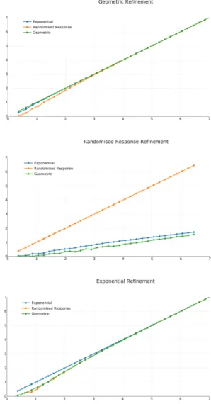
We examine this question experimentally by considering different mechanisms and investigating for which values of ε average-case refinement holds. For simplicity of presentation, we show results for 5 × 5 matrices, noting that we observed similar results for experiments across different matrix dimen-sions. 20 The results are plotted in Figure1.
The plots show the relationship between ε1(x-axis) and ε2
(y-axis) where ε1 parametrizes the mechanism being refined
and ε2 parametrizes the refining mechanism. For example,
the blue line on the top graph represents T Gε1 vavg Eε2.
We fix ε1 and ask for what value of ε2 do we get a vavg
refinement? Notice that the line ε1 = ε2 corresponds to the
same mechanism in both axes (since every mechanism refines itself).
We can see that refining the randomized response mech-anism requires much smaller values of epsilon in the other
18Although we note that our result for the exponential mechanism is only a conjecture.
19As with the previous theorem, note that the results for the exponential mechanism are stated as conjecture only, and this conjecture is assumed in the statement of this corollary.
20By similar results, we mean wrt the coarse-grained comparison of plots that we do here.
Fig. 1. Refinement of mechanisms under vavg for 5 × 5 channels. The x-axis (ε1) represents the mechanism on the LHS of the relation. The y-x-axis (ε2) represents the refining mechanism. We fix ε1 and ask for what value of ε2 do we get a vavg refinement? The top graph represents refinement of the truncated geometric mechanism (that is, T G vavg), the middle graph is refinement of randomized response (R vavg), and the bottom graph is refinement of the exponential mechanism (E vavg).
mechanisms. For example, from the middle graph we can see that R4vavgT G1 (approximately) whereas from the top
graph we have T G4 vavg R4. This means that the
random-ized response mechanism is very ‘safe’ against average-case adversaries compared with the other mechanisms, as it is much more ‘difficult’ to refine than the other mechanisms.
We also notice that for ‘large’ values of ε1, the exponential
and geometric mechanisms refine each other for approximately the same ε2 values. This suggests that for these values, the
epsilons are comparable (that is, the mechanisms are equally ‘safe’ for similar values of ε). However, smaller values of ε1 require a (relatively) large reduction in ε2 to obtain a