HAL Id: hal-01957704
https://hal.archives-ouvertes.fr/hal-01957704
Submitted on 17 Dec 2018
HAL is a multi-disciplinary open access
archive for the deposit and dissemination of
sci-entific research documents, whether they are
pub-lished or not. The documents may come from
teaching and research institutions in France or
abroad, or from public or private research centers.
L’archive ouverte pluridisciplinaire HAL, est
destinée au dépôt et à la diffusion de documents
scientifiques de niveau recherche, publiés ou non,
émanant des établissements d’enseignement et de
recherche français ou étrangers, des laboratoires
publics ou privés.
The Dynamics of Learning: A Random Matrix Approach
Zhenyu Liao, Romain Couillet
To cite this version:
Zhenyu Liao, Romain Couillet. The Dynamics of Learning: A Random Matrix Approach. ICML 2018
- 35th International Conference on Machine Learning, Jul 2018, Stockholm, Sweden. �hal-01957704�
The Dynamics of Learning: A Random Matrix Approach
Zhenyu Liao1 Romain Couillet1 2
Abstract
Understanding the learning dynamics of neural networks is one of the key issues for the improve-ment of optimization algorithms as well as for the theoretical comprehension of why deep neu-ral nets work so well today. In this paper, we introduce a random matrix-based framework to analyze the learning dynamics of a single-layer linear network on a binary classification problem, for data of simultaneously large dimension and size, trained by gradient descent. Our results pro-vide rich insights into common questions in neural nets, such as overfitting, early stopping and the initialization of training, thereby opening the door for future studies of more elaborate structures and models appearing in today’s neural networks.
1. Introduction
Deep neural networks trained with backpropagation have commonly attained superhuman performance in applica-tions of computer vision (Krizhevsky et al.,2012) and many others (Schmidhuber,2015) and are thus receiving an un-precedented research interest. Despite the rapid growth of the list of successful applications with these gradient-based methods, our theoretical understanding, however, is progressing at a more modest pace.
One of the salient features of deep networks today is that they often have far more model parameters than the number of training samples that they are trained on, but meanwhile some of the models still exhibit remarkably good general-ization performance when applied to unseen data of similar nature, while others generalize poorly in exactly the same setting. A satisfying explanation of this phenomenon would be the key to more powerful and reliable network structures.
1Laboratoire des Signaux et Syst`emes (L2S), CentraleSup´elec,
Universit´e Paris-Saclay, France;2G-STATS Data Science Chair,
GIPSA-lab, University Grenobles-Alpes, France. Correspondence to: Zhenyu Liao <[email protected]>, Romain Couillet <[email protected]>.
Proceedings of the 35thInternational Conference on Machine
Learning, Stockholm, Sweden, PMLR 80, 2018. Copyright 2018 by the author(s).
To answer such a question, statistical learning theory has proposed interpretations from the viewpoint of system com-plexity (Vapnik,2013;Bartlett & Mendelson,2002;Poggio et al.,2004). In the case of large numbers of parameters, it is suggested to apply some form of regularization to ensure good generalization performance. Regularizations can be explicit, such as the dropout technique (Srivastava et al.,
2014) or the l2-penalization (weight decay) as reported in
(Krizhevsky et al.,2012); or implicit, as in the case of the early stopping strategy (Yao et al.,2007) or the stochastic gradient descent algorithm itself (Zhang et al.,2016). Inspired by the recent line of works (Saxe et al.,2013; Ad-vani & Saxe,2017), in this article we introduce a random matrix framework to analyze the training and, more impor-tantly, the generalization performance of neural networks, trained by gradient descent. Preliminary results established from a toy model of two-class classification on a single-layer linear network are presented, which, despite their simplicity, shed new light on the understanding of many important as-pects in training neural nets. In particular, we demonstrate how early stopping can naturally protect the network against overfitting, which becomes more severe as the number of training sample approaches the dimension of the data. We also provide a strict lower bound on the training sample size for a given classification task in this simple setting. A byproduct of our analysis implies that random initialization, although commonly used in practice in training deep net-works (Glorot & Bengio,2010;Krizhevsky et al.,2012), may lead to a degradation of the network performance. From a more theoretical point of view, our analyses allow one to evaluate any functional of the eigenvalues of the sample covariance matrix of the data (or of the data rep-resentation learned from previous layers in a deep model), which is at the core of understanding many experimental observations in today’s deep networks (Glorot & Bengio,
2010;Ioffe & Szegedy,2015). Our results are envisioned to generalize to more elaborate settings, notably to deeper models that are trained with the stochastic gradient descent algorithm, which is of more practical interest today due to the tremendous size of the data.
Notations: Boldface lowercase (uppercase) characters stand for vectors (matrices), and non-boldface for scalars respec-tively. 0pis the column vector of zeros of size p, and Ip
The Dynamics of Learning: A Random Matrix Approach
the p ⇥ p identity matrix. The notation (·)Tdenotes the
transpose operator. The norm k · k is the Euclidean norm for vectors and the operator norm for matrices. =(·) denotes the imaginary part of a complex number. For x 2 R, we denote for simplicity (x)+
⌘ max(x, 0).
In the remainder of the article, we introduce the problem of interest and recall the results of (Saxe et al.,2013) in Section2. After a brief overview of basic concepts and methods to be used throughout the article in Section3, our main results on the training and generalization performance of the network are presented in Section4, followed by a thorough discussion in Section5and experiments on the popular MNIST database (LeCun et al.,1998) in Section6. Section7concludes the article by summarizing the main results and outlining future research directions.
2. Problem Statement
Let the training data x1, . . . , xn2 Rpbe independent
vec-tors drawn from two distribution classes C1and C2of
car-dinality n1and n2(thus n1+ n2 = n), respectively. We
assume that the data vector xiof class Cacan be written as
xi= ( 1)aµ + zi
for a = {1, 2}, with µ 2 Rp and z
i a Gaussian random
vector zi⇠ N (0p, Ip). In the context of a binary
classifica-tion problem, one takes the label yi= 1for xi2 C1and
yj = 1for xj 2 C2to distinguish the two classes.
We denote the training data matrix X = ⇥x1, . . . , xn⇤ 2
Rp⇥nby cascading all x
i’s as column vectors and associated
label vector y 2 Rn. With the pair {X, y}, a classifier is
trained using “full-batch” gradient descent to minimize the loss function L(w) given by
L(w) = 1 2nky
T wTXk2
so that for a new datum ˆx, the output of the classifier is ˆ
y = wTx, the sign of which is then used to decide the classˆ
of ˆx. The derivative of L with respective to w is given by @L(w)
@w = 1
nX(y X
Tw).
The gradient descent algorithm (Boyd & Vandenberghe,
2004) takes small steps of size ↵ along the opposite direction of the associated gradient, i.e., wt+1= wt ↵@L(w)@w w=w
t.
Following the previous works of (Saxe et al.,2013;Advani & Saxe,2017), when the learning rate ↵ is small, wt+1
and wt are close to each other so that by performing a
continuous-time approximation, one obtains the following differential equation @w(t) @t = ↵ @L(w) @w = ↵ nX y X Tw(t)
the solution of which is given explicitly by
w(t) = e ↵tnXXTw0+ ⇣ Ip e ↵t nXXT ⌘ (XXT) 1Xy (1) if one assumes that XXT is invertible (only possible in
the case p < n), with w0 ⌘ w(t = 0) the
initializa-tion of the weight vector; we recall the definiinitializa-tion of the exponential of a matrix 1
nXXT given by the power
se-ries e1 nXXT = P1 k=0k!1( 1 nXXT)k = Ve⇤VT, with the eigendecomposition of 1 nXXT = V⇤VTand e ⇤is a
di-agonal matrix with elements equal to the exponential of the elements of ⇤. As t ! 1 the network “forgets” the initialization w0 and results in the least-square solution
wLS⌘ (XXT) 1Xy.
When p > n, XXTis no longer invertible. Assuming XTX
is invertible and writing Xy = XXT X XTX 1y, the
solution is similarly given by
w(t) = e ↵tnXXTw 0+ X ⇣ In e ↵t nXTX ⌘ (XTX) 1y
with the least-square solution wLS⌘ X(XTX) 1y.
In the work of (Advani & Saxe,2017) it is assumed that Xhas i.i.d. entries and that there is no linking structure between the data and associated targets in such a way that the “true” weight vector ¯w to be learned is independent of X so as to simplify the analysis. In the present work we aim instead at exploring the capacity of the network to retrieve the (mixture modeled) data structure and position ourselves in a more realistic setting where w captures the different statistical structures (between classes) of the pair (X, y). Our results are thus of more guiding significance
for practical interests. From (1) note that both e ↵t
nXXT and Ip e ↵tnXXTshare
the same eigenvectors with the sample covariance matrix
1
nXXT, which thus plays a pivotal role in the network
learn-ing dynamics. More concretely, the projections of w0and
wLS onto the eigenspace of n1XXT, weighted by
func-tions (exp( ↵t i)or 1 exp( ↵t i)) of the associated
eigenvalue i, give the temporal evolution of w(t) and
con-sequently the training and generalization performance of the network. The core of our study therefore consists in deeply understanding of the eigenpairs of this sample covariance matrix, which has been largely investigated in the random matrix literature (Bai & Silverstein,2010).
3. Preliminaries
Throughout this paper, we will be relying on some basic yet powerful concepts and methods from random matrix theory, which shall be briefly highlighted in this section.
The Dynamics of Learning: A Random Matrix Approach
3.1. Resolvent and deterministic equivalents
Consider an n ⇥ n Hermitian random matrix M. We define its resolvent QM(z), for z 2 C not an eigenvalue of M, as
QM(z) = (M zIn) 1.
Through the Cauchy integral formula discussed in the fol-lowing subsection, as well as its central importance in ran-dom matrix theory, Q1
nXXT(z)is the key object investigated
in this article.
For certain simple distributions of M, one may define a so-called deterministic equivalent (Hachem et al., 2007;
Couillet & Debbah, 2011) ¯QM for QM, which is a
de-terministic matrix such that for all A 2 Rn⇥n and all
a, b 2 Rn of bounded (spectral and Euclidean,
respec-tively) norms, 1
ntr (AQM) 1
ntr A ¯QM ! 0 and
aT Q
M Q¯M b! 0 almost surely as n ! 1. As such,
deterministic equivalents allow to transfer random spectral properties of M in the form of deterministic limiting quan-tities and thus allows for a more detailed investigation. 3.2. Cauchy’s integral formula
First note that the resolvent QM(z)has the same eigenspace
as M, with associated eigenvalue ireplaced by i1z. As
discussed at the end of Section2, our objective is to evalu-ate functions of these eigenvalues, which reminds us of the fundamental Cauchy’s integral formula, stating that for any function f holomorphic on an open subset U of the complex plane, one can compute f( ) by contour integration. More concretely, for a closed positively (counter-clockwise) ori-ented path in U with winding number one (i.e., describing a 360 rotation), one has, for contained in the surface de-scribed by , 1 2⇡i H f (z) z dz = f ( )and 1 2⇡i H f (z) z dz = 0
if lies outside the contour of .
With Cauchy’s integral formula, one is able to evaluate more sophisticated functionals of the random matrix M. For example, for f(M) ⌘ aTeMbone has
f (M) = 1 2⇡i
I
exp(z)aTQM(z)b dz
with a positively oriented path circling around all the eigenvalues of M. Moreover, from the previous subsection one knows that the bilinear form aTQ
M(z)bis
asymptot-ically close to a non-random quantity aTQ¯M(z)b. One thus deduces that the functional aTeMb has an
asymp-totically deterministic behavior that can be expressed as
1 2⇡i
H
exp(z)aTQ¯M(z)b dz.
This observation serves in the present article as the foun-dation for the performance analysis of the gradient-based classifier, as described in the following section.
4. Temporal Evolution of Training and
Generalization Performance
With the explicit expression of w(t) in (1), we now turn our attention to the training and generalization performances of the classifier as a function of the training time t. To this end, we shall be working under the following assumptions. Assumption 1 (Growth Rate). As n ! 1,
1. p
n ! c 2 (0, 1).
2. For a = {1, 2}, na
n ! ca2 (0, 1).
3. kµk = O(1).
The above assumption ensures that the matrix 1
nXXTis of
bounded operator norm for all large n, p with probability one (Bai & Silverstein,1998).
Assumption 2 (Random Initialization). Let w0⌘ w(t =
0)be a random vector with i.i.d. entries of zero mean, vari-ance 2/pfor some > 0 and finite fourth moment.
We first focus on the generalization performance, i.e., the average performance of the trained classifier taking as input an unseen new datum ˆx drawn from class C1or C2.
4.1. Generalization Performance
To evaluate the generalization performance of the classifier, we are interested in two types of misclassification rates, for a new datum ˆx drawn from class C1or C2, as
P(w(t)Tx > 0ˆ | ˆx 2 C1), P(w(t)Tx < 0ˆ | ˆx 2 C2).
Since the new datum ˆx is independent of w(t), w(t)Txˆis a
Gaussian random variable of mean ±w(t)Tµand variance
kw(t)k2. The above probabilities can therefore be given via
the Q-function: Q(x) ⌘ p1 2⇡ R1 x exp ⇣ u2 2 ⌘ du. We thus resort to the computation of w(t)Tµas well as w(t)Tw(t)
to evaluate the aforementioned classification error. For µTw(t), with Cauchy’s integral formula we have
µTw(t) = µTe ↵tnXX T w0+ µT ⇣ Ip e ↵t nXX T⌘ wLS = 1 2⇡i I ft(z)µT ✓1 nXX T zI p ◆ 1 w0dz 1 2⇡i I 1 f t(z) z µ T✓1 nXX T zI p ◆ 1 1 nXy dz with ft(z)⌘ exp( ↵tz), for a positive closed path
cir-cling around all eigenvalues of 1
nXXT. Note that the data
matrix X can be rewritten as
The Dynamics of Learning: A Random Matrix Approach
with Z ⌘ ⇥z1, . . . , zn⇤ 2 Rp⇥n of i.i.d. N (0, 1) entries
and ja 2 Rn the canonical vectors of class Ca such that
(ja)i= xi2Ca. To isolate the deterministic vectors µ and
ja’s from the random Z in the expression of µTw(t), we
exploit Woodbury’s identity to obtain ✓1 nXX T zI p ◆ 1 = Q(z) Q(z)⇥µ n1Zy⇤ µTQ(z)µ 1 + 1 nµTQ(z)Zy ⇤ 1 + 1 nyTZTQ(z) 1 nZy 1 µT 1 nyTZT Q(z)
where we denote the resolvent Q(z) ⌘ 1
nZZT zIp 1
, a deterministic equivalent of which is given by
Q(z)$ ¯Q(z)⌘ m(z)Ip
with m(z) determined by the popular Marˇcenko–Pastur equation (Marˇcenko & Pastur,1967)
m(z) = 1 c z 2cz +
p
(1 c z)2 4cz
2cz (2)
where the branch of the square root is selected in such a way that =(z) · =m(z) > 0, i.e., for a given z there exists a unique corresponding m(z).
Substituting Q(z) by the simple form deterministic equiv-alent m(z)Ip, we are able to estimate the random
vari-able µTw(t)with a contour integral of some deterministic
quantities as n, p ! 1. Similar arguments also hold for w(t)Tw(t), together leading to the following theorem.
Theorem 1 (Generalization Performance). Let Assump-tions1and2hold. As n ! 1, with probability one
P(w(t)Tx > 0ˆ | ˆx 2 C1) Q ✓ E p V ◆ ! 0 P(w(t)Tx < 0ˆ | ˆx 2 C2) Q ✓ E p V ◆ ! 0 where E⌘ 1 2⇡i I 1 f t(z) z kµk2m(z) dz (kµk2+ c) m(z) + 1 V ⌘ 1 2⇡i I " 1 z2(1 ft(z))2 (kµk2+ c) m(z) + 1 2f2 t(z)m(z) # dz
with a closed positively oriented path that contains all eigenvalues of 1
nXXTand the origin, ft(z)⌘ exp( ↵tz)
and m(z) given by Equation (2).
Although derived from the case p < n, Theorem1also applies when p > n. To see this, note that with Cauchy’s integral formula, for z 6= 0 not an eigenvalue of 1
nXXT (thus not of 1 nXTX), one has X 1 nXTX zIn 1 y = 1 nXXT zIp 1
Xy, which further leads to the same ex-pressions as in Theorem1. Since 1
nXXTand 1
nXTXhave
the same eigenvalues except for additional zero eigenvalues for the larger matrix, the path remains unchanged (as we demand that contains the origin) and hence Theorem1
holds true for both p < n and p > n. The case p = n can be obtained by continuity arguments.
4.2. Training performance
To compare generalization versus training performance, we are now interested in the behavior of the classifier when applied to the training set X. To this end, we consider the random vector XTw(t)given by
XTw(t) = XTe ↵tnXXTw0+XT ⇣ Ip e ↵t nXXT ⌘ wLS.
Note that the i-th entry of XTw(t)is given by the bilinear
form eT
iXTw(t), with eithe canonical vector with unique
non-zero entry [ei]i= 1. With previous notations we have
eTiXTw(t) = 1 2⇡i I ft(z, t)eTiXT ✓1 nXX T zI p ◆ 1 w0dz 1 2⇡i I 1 f t(z) z e T i 1 nX T ✓1 nXX T zI p ◆ 1 Xy dz which yields the following results.
Theorem 2 (Training Performance). Under the assumptions and notations of Theorem1, as n ! 1,
P(w(t)Txi> 0| xi2 C1) Q E⇤ p V⇤ E2 ⇤ ! ! 0 P(w(t)Txi< 0| xi2 C2) Q p E⇤ V⇤ E2⇤ ! ! 0
almost surely, with
E⇤⌘ 1 2⇡i I 1 f t(z) z dz (kµk2+ c) m(z) + 1 V⇤⌘ 1 2⇡i I " 1 z(1 ft(z)) 2 (kµk2+ c) m(z) + 1 2f2 t(z)zm(z) # dz.
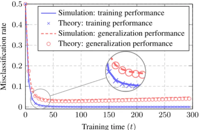
In Figure1we compare finite dimensional simulations with theoretical results obtained from Theorem1and2and ob-serve a very close match, already for not too large n, p. As t grows large, the generalization error first drops rapidly with the training error, then goes up, although slightly, while the training error continues to decrease to zero. This is because the classifier starts to over-fit the training data
The Dynamics of Learning: A Random Matrix Approach 0 50 100 150 200 250 300 0 0.1 0.2 0.3 0.4 0.5 Training time (t) Misclassification rate
Simulation: training performance Theory: training performance
Simulation: generalization performance Theory: generalization performance
0
50
100
150
200
250
300
0
0.1
0.2
0.3
0.4
0.5
Training time (t)
Misclassification
rate
Simulation: training performance
Theory: training performance
Simulation: generalization performance
Theory: generalization performance
Figure 1. Training and generalization performance for µ = [2; 0p 1], p = 256, n = 512, 2 = 0.1, ↵ = 0.01 and
c1= c2= 1/2. Results obtained by averaging over 50 runs.
X and performs badly on unseen ones. To avoid over-fitting, one effectual approach is to apply regularization strategies (Bishop,2007), for example, to “early stop” (at t = 100 for instance in the setting of Figure 1) in the training process. However, this introduces new hyperpa-rameters such as the optimal stopping time toptthat is of
crucial importance for the network performance and is often tuned through cross-validation in practice. Theorem1and2
tell us that the training and generalization performances, although being random themselves, have asymptotically deterministic behaviors described by (E⇤, V⇤)and (E, V ),
respectively, which allows for a deeper understanding on the choice of topt, since E, V are in fact functions of t via
ft(z)⌘ exp( ↵tz).
Nonetheless, the expressions in Theorem1and2of contour integrations are not easily analyzable nor interpretable. To gain more insight, we shall rewrite (E, V ) and (E⇤, V⇤)
in a more readable way. First, note from Figure 2that the matrix 1
nXXThas (possibly) two types of eigenvalues:
those inside the main bulk (between ⌘ (1 pc)2and +⌘ (1 +pc)2) of the Marˇcenko–Pastur distribution
⌫(dx) = p (x )+( + x)+ 2⇡cx dx + ✓ 1 1 c ◆+ (x) (3) and a (possibly) isolated one1 lying away from [ ,
+],
that shall be treated separately. We rewrite the path (that contains all eigenvalues of 1
nXXT) as the sum of two paths
1The existence (or absence) of outlying eigenvalues for the
sample covariance matrix has been largely investigated in the random matrix literature and is related to the so-called “spiked random matrix model”. We refer the reader to (Benaych-Georges & Nadakuditi,2011) for an introduction. The information carried by these “isolated” eigenpairs also marks an important technical difference to (Advani & Saxe,2017) in which X is only composed of noise terms.
band s, that circle around the main bulk and the isolated
eigenvalue (if any), respectively. To handle the first integral of b, we use the fact that for any nonzero 2 R, the limit
limz2Z! m(z)⌘ ˇm( )exists (Silverstein & Choi,1995)
and follow the idea in (Bai & Silverstein,2008) by choosing the contour b to be a rectangle with sides parallel to the
axes, intersecting the real axis at 0 and +and the horizontal
sides being a distance " ! 0 away from the real axis, to split the contour integral into four single ones of ˇm(x). The second integral circling around scan be computed with
the residue theorem. This together leads to the expressions of (E, V ) and (E⇤, V⇤)as follows2
E = Z 1 f t(x) x µ(dx) (4) V = kµk 2+ c kµk2 Z (1 f t(x))2µ(dx) x2 + 2Z f2 t(x)⌫(dx) (5) E⇤= kµk 2+ c kµk2 Z 1 f t(x) x µ(dx) (6) V⇤= kµk 2+ c kµk2 Z (1 f t(x))2µ(dx) x + 2Z xf2 t(x)⌫(dx) (7) where we recall ft(x) = exp( ↵tx), ⌫(x) given by (3) and
denote the measure
µ(dx)⌘ p (x )+( + x)+ 2⇡( s x) dx+(kµk 4 c)+ kµk2 s(x) (8) as well as s= c + 1 +kµk2+ c kµk2 ( p c + 1)2 (9) with equality if and only if kµk2=pc.
A first remark on the expressions of (4)-(7) is that E⇤differs
from E only by a factor of kµk2+c
kµk2 . Also, both V and V⇤
are the sum of two parts: the first part that strongly depends on µ and the second one that is independent of µ. One thus deduces for kµk ! 0 that E ! 0 and
V ! Z (1 f t(x))2 x2 ⇢(dx) + 2Z f2 t(x)⌫(dx) > 0 with ⇢(dx) ⌘ p(x )+( + x)+
2⇡(c+1) dxand therefore the
gen-eralization performance goes to Q(0) = 0.5. On the other hand, for kµk ! 1, one has pE
V ! 1 and hence the
classifier makes perfect predictions.
In a more general context (i.e., for Gaussian mixture mod-els with generic means and covariances as investigated in
2We defer the readers to SectionAin Supplementary Material
The Dynamics of Learning: A Random Matrix Approach
(Benaych-Georges & Couillet,2016), and obviously for practical datasets), there may be more than one eigenvalue of 1
nXXTlying outside the main bulk, which may not be
limited to the interval [ , +]. In this case, the expression
of m(z), instead of being explicitly given by (2), may be determined through more elaborate (often implicit) formula-tions. While handling more generic models is technically reachable within the present analysis scheme, the results are much less intuitive. Similar objectives cannot be achieved within the framework presented in (Advani & Saxe,2017); this conveys more practical interest to our results and the proposed analysis framework.
0 1 2 3 4 Eigenvalues of 1 nXX T Marˇcenko–Pastur distribution Theory: sgiven in (9)
0
1
2
3
4
Eigenvalues of
1
n
XX
T
Marˇcenko–Pastur distribution
Theory:
s
given in (
9
)
Figure 2. Eigenvalue distribution of 1 nXX
Tfor µ = [1.5; 0 p 1],
p = 512, n = 1 024 and c1= c2 = 1/2.
5. Discussions
In this section, with a careful inspection of (4) and (5), dis-cussions will be made from several different aspects. First of all, recall that the generalization performance is simply given by Q⇣µTw(t)
kw(t)k
⌘
, with the term µTw(t)
kw(t)k describing the
alignment between w(t) and µ, therefore the best possible generalization performance is simply Q(kµk). Nonetheless, this “best” performance can never be achieved as long as p/n! c > 0, as described in the following remark. Remark 1 (Optimal Generalization Performance). Note that, with Cauchy–Schwarz inequality and the fact that R
µ(dx) =kµk2from (8), one has
E2 Z (1 f t(x))2 x2 dµ(x)· Z dµ(x) kµk 4 kµk2+ cV
with equality in the right-most inequality if and only if the variance 2 = 0. One thus concludes that E/pV
kµk2/p
kµk2+ cand the best generalization performance
(lowest misclassification rate) is Q(kµk2/p
kµk2+ c)and
can be attained only when 2= 0.
The above remark is of particular interest because, for a given task (thus p, µ fixed) it allows one to compute the
minimum training data number n to fulfill a certain request of classification accuracy.
As a side remark, note that in the expression of E/pV the initialization variance 2only appears in V , meaning
that random initializations impair the generalization perfor-mance of the network. As such, one should initialize with
2very close, but not equal, to zero, to obtain symmetry
breaking between hidden units (Goodfellow et al.,2016) as well as to mitigate the drop of performance due to large 2.
In Figure3we plot the optimal generalization performance with the corresponding optimal stopping time as functions of 2, showing that small initialization helps training in
terms of both accuracy and efficiency.
103 2 10 1 100 4 5 6 7 8 ·10 2 2
Optimal error rates
100 2 10 1 100
200 400 600
2
Optimal stopping time
Figure 3. Optimal performance and corresponding stopping time as functions of 2, with c = 1/2, kµk2= 4and ↵ = 0.01.
Although the integrals in (4) and (5) do not have nice closed forms, note that, for t close to 0, with a Taylor expansion of ft(x)⌘ exp( ↵tx) around ↵tx = 0, one gets more
inter-pretable forms of E and V without integrals, as presented in the following subsection.
5.1. Approximation for t close to 0
Taking t = 0, one has ft(x) = 1and therefore E = 0,
V = 2R ⌫(dx) = 2, with ⌫(dx) the Marˇcenko–Pastur
distribution given in (3). As a consequence, at the beginning stage of training, the generalization performance is Q(0) = 0.5for 26= 0 and the classifier makes random guesses.
For t not equal but close to 0, the Taylor expansion of ft(x)⌘ exp( ↵tx) around ↵tx = 0 gives
ft(x)⌘ exp( ↵tx) ⇡ 1 ↵tx + O(↵2t2x2).
Making the substitution x = 1 + c 2pc cos ✓ and with the fact thatR⇡
0 sin2✓ p+q cos ✓d✓ = p⇡ q2 ⇣ 1 p1 q2/p2⌘(see
for example 3.644-5 in (Gradshteyn & Ryzhik,2014)), one gets E = ˜E + O(↵2t2)and V = ˜V + O(↵2t2), where
˜
E⌘↵t2 g(µ, c) +(kµk
4 c)+
kµk2 ↵t =kµk 2↵t
The Dynamics of Learning: A Random Matrix Approach ˜ V ⌘ kµk 2+ c kµk2 (kµk4 c)+ kµk2 ↵ 2t2+kµk2+ c kµk2 ↵2t2 2 g(µ, c) + 2(1 + c)↵2t2 2 2↵t + ✓ 1 1 c ◆+ 2 + 2 2c 1 + c (1 + p c)|1 pc| = (kµk2+ c + c 2)↵2t2+ 2(↵t 1)2 with g(µ, c) ⌘ kµk2+ c kµk2 ⇣ kµk +kµkpc ⌘ kµk kµkpc and consequently 1 2g(µ, c) + (kµk4 c)+ kµk2 = kµk2. It is
interesting to note from the above calculation that, although Eand V seem to have different behaviors3for kµk2>pc
or c > 1, it is in fact not the case and the extra part of kµk2>pc(or c > 1) compensates for the singularity of
the integral, so that the generalization performance of the classifier is a smooth function of both kµk2and c.
Taking the derivative of pE˜ ˜
V with respect to t, one has
@ @t ˜ E p ˜ V = ↵(1 ↵t) 2 ˜ V3/2
which implies that the maximum ofpE˜ ˜ V is
kµk2
p
kµk2+c+c 2
and can be attained with t = 1/↵. Moreover, taking t = 0 in the above equation one gets @
@t ˜ E p ˜ V t=0= ↵. Therefore,
large is harmful to the training efficiency, which coincides with the conclusion from Remark1.
The approximation error arising from Taylor expansion can be large for t away from 0, e.g., at t = 1/↵ the difference E E˜is of order O(1) and thus cannot be neglected. 5.2. As t ! 1: least-squares solution
As t ! 1, one has ft(x) ! 0 which results in the
least-square solution wLS = (XXT) 1Xy or wLS = X(XTX) 1yand consequently µTw LS kwLSk = kµk 2 p kµk2+ c s 1 min ✓ c,1 c ◆ . (10)
Comparing (10) with the expression in Remark1, one ob-serves that when t ! 1 the network becomes “over-trained” and the performance drops by a factor ofp1 min(c, c 1).
This becomes even worse when c gets close to 1, as is con-sistent with the empirical findings in (Advani & Saxe,2017). However, the point c = 1 is a singularity for (10), but not for
E p
V as in (4) and (5). One may thus expect to have a smooth
and reliable behavior of the well-trained network for c close
3This phenomenon has been largely observed in random matrix
theory and is referred to as “phase transition”(Baik et al.,2005).
to 1, which is a noticeable advantage of gradient-based training compared to simple least-square method. This co-incides with the conclusion of (Yao et al.,2007) in which the asymptotic behavior of solely n ! 1 is considered. In Figure4we plot the generalization performance from simulation (blue line), the approximation from Taylor ex-pansion of ft(x)as described in Section5.1(red dashed
line), together with the performance of wLS(cyan dashed
line). One observes a close match between the result from Taylor expansion and the true performance for t small, with the former being optimal at t = 100 and the latter slowly approaching the performance of wLSas t goes to infinity.
In Figure5we underline the case c = 1 by taking p = n = 512 with all other parameters unchanged from Figure4. One observes that the simulation curve (blue line) increases much faster compared to Figure4and is supposed to end up at 0.5, which is the performance of wLS(cyan dashed
line). This confirms a serious degradation of performance for c close to 1 of the classical least-squares solution.
0 200 400 600 800 1,000 0 0.1 0.2 0.3 0.4 0.5 Training time (t) Misclassification rate Simulation
Approximation via Taylor expansion Performance of wLS
0
200
400
600
800
1,000
0
0.1
0.2
0.3
0.4
0.5
Training time (t)
Misclassification
rate
Simulation
Approximation via Taylor expansion
Performance of w
LS
Figure 4. Generalization performance for µ = ⇥2; 0p 1⇤, p =
256, n = 512, c1 = c2 = 1/2, 2 = 0.1and ↵ = 0.01.
Simula-tion results obtained by averaging over 50 runs.
5.3. Special case for c = 0
One major interest of random matrix analysis is that the ratio cappears constantly in the analysis. Taking c = 0 signifies that we have far more training data than their dimension. This results in both , +! 1, s! 1 + kµk2and
E! kµk21 ft(1 +kµk2) 1 +kµk2 V ! kµk2 ✓1 f t(1 +kµk2) 1 +kµk2 ◆2 + 2ft2(1). As a consequence, pE V ! kµk if 2 = 0. This can be
The Dynamics of Learning: A Random Matrix Approach 0 200 400 600 800 1,000 0.1 0.2 0.3 0.4 0.5 Training time (t) Misclassification rate Simulation
Approximation via Taylor expansion Performance of wLS
Figure 5. Generalization performance for µ = ⇥2; 0p 1⇤, p =
512, n = 512, c1= c2 = 1/2, 2= 0.1and ↵ = 0.01.
Simula-tion results obtained by averaging over 50 runs.
classifier learns to align perfectly to µ so thatµTw(t)
kw(t)k =kµk.
On the other hand, with initialization 2
6= 0, one always has pE
V < kµk. But still, as t goes large, the network
forgets the initialization exponentially fast and converges to the optimal w(t) that aligns to µ.
In particular, for 2
6= 0, we are interested in the optimal stopping time by taking the derivative with respect to t,
@ @t E p V = ↵ 2 kµk2 V3/2 kµk2f t(1 +kµk2) + 1 1 +kµk2 f 2 t(1) > 0
showing that when c = 0, the generalization performance continues to increase as t grows and there is in fact no “over-training” in this case.
0 50 100 150 200 250 300 0 0.1 0.2 0.3 0.4 0.5 Training time (t) Misclassification rate
Simulation: training performance Theory: training performance
Simulation: generalization performance Theory: generalization performance
0
50
100
150
200
250
300
0
0.1
0.2
0.3
0.4
0.5
Training time (t)
Misclassification
rate
Simulation: training performance
Theory: training performance
Simulation: generalization performance
Theory: generalization performance
Figure 6. Training and generalization performance for MNIST data (number 1 and 7) with n = p = 784, c1= c2 = 1/2, ↵ = 0.01
and 2= 0.1. Results obtained by averaging over 100 runs.
6. Numerical Validations
We close this article with experiments on the popular MNIST dataset (LeCun et al.,1998) (number 1 and 7). We randomly select training sets of size n = 784 vectorized images of dimension p = 784 and add artificially a Gaus-sian white noise of 10dB in order to be more compliant with our toy model setting. Empirical means and covari-ances of each class are estimated from the full set of 13 007 MNIST images (6 742 images of number 1 and 6 265 of number 7). The image vectors in each class are whitened by pre-multiplying C 1/2
a and re-centered to have means of
±µ, with µ half of the difference between means from the two classes. We observe an extremely close fit between our results and the empirical simulations, as shown in Figure6.
7. Conclusion
In this article, we established a random matrix approach to the analysis of learning dynamics for gradient-based al-gorithms on data of simultaneously large dimension and size. With a toy model of Gaussian mixture data with ±µ means and identity covariance, we have shown that the train-ing and generalization performances of the network have asymptotically deterministic behaviors that can be evaluated via so-called deterministic equivalents and computed with complex contour integrals (and even under the form of real integrals in the present setting). The article can be gener-alized in many ways: with more generic mixture models (with the Gaussian assumption relaxed), on more appro-priate loss functions (logistic regression for example), and more advanced optimization methods.
In the present work, the analysis has been performed on the “full-batch” gradient descent system. However, the most popular method used today is in fact its “stochastic” version (Bottou,2010) where only a fixed-size (nbatch) randomly
selected subset (called a mini-batch) of the training data is used to compute the gradient and descend one step along with the opposite direction of this gradient in each iteration. In this scenario, one of major concern in practice lies in determining the optimal size of the mini-batch and its in-fluence on the generalization performance of the network (Keskar et al.,2016). This can be naturally linked to the ratio nbatch/pin the random matrix analysis.
Deep networks that are of more practical interests, however, need more efforts. As mentioned in (Saxe et al.,2013; Ad-vani & Saxe,2017), in the case of multi-layer networks, the learning dynamics depend, instead of each eigenmode separately, on the coupling of different eigenmodes from different layers. To handle this difficulty, one may add extra assumptions of independence between layers as in ( Choro-manska et al.,2015) so as to study each layer separately and then reassemble to retrieve the results of the whole network.
The Dynamics of Learning: A Random Matrix Approach
Acknowledgments
We thank the anonymous reviewers for their comments and constructive suggestions. We would like to acknowledge this work is supported by the ANR Project RMT4GRAPH (ANR-14-CE28-0006) and the Project DeepRMT of La Fondation Sup´elec.
References
Advani, M. S. and Saxe, A. M. High-dimensional dynamics of generalization error in neural networks. arXiv preprint arXiv:1710.03667, 2017.
Bai, Z. and Silverstein, J. W. Spectral analysis of large di-mensional random matrices, volume 20. Springer, 2010. Bai, Z.-D. and Silverstein, J. W. No eigenvalues outside the support of the limiting spectral distribution of large-dimensional sample covariance matrices. Annals of prob-ability, pp. 316–345, 1998.
Bai, Z. D. and Silverstein, J. W. CLT for linear spectral statis-tics of large-dimensional sample covariance matrices. In Advances In Statistics, pp. 281–333. World Scientific, 2008.
Baik, J., Arous, G. B., P´ech´e, S., et al. Phase transition of the largest eigenvalue for nonnull complex sample covariance matrices. The Annals of Probability, 33(5): 1643–1697, 2005.
Bartlett, P. L. and Mendelson, S. Rademacher and gaussian complexities: Risk bounds and structural results. Journal of Machine Learning Research, 3(Nov):463–482, 2002. Benaych-Georges, F. and Couillet, R. Spectral analysis of
the gram matrix of mixture models. ESAIM: Probability and Statistics, 20:217–237, 2016.
Benaych-Georges, F. and Nadakuditi, R. R. The eigenvalues and eigenvectors of finite, low rank perturbations of large random matrices. Advances in Mathematics, 227(1):494– 521, 2011.
Billingsley, P. Probability and measure. John Wiley & Sons, 2008.
Bishop, C. M. Pattern Recognition and Machine Learning. Springer, 2007.
Bottou, L. Large-scale machine learning with stochastic gradient descent. In Proceedings of COMPSTAT’2010, pp. 177–186. Springer, 2010.
Boyd, S. and Vandenberghe, L. Convex optimization. Cam-bridge university press, 2004.
Choromanska, A., Henaff, M., Mathieu, M., Arous, G. B., and LeCun, Y. The loss surfaces of multilayer networks. In Artificial Intelligence and Statistics, pp. 192–204, 2015.
Couillet, R. and Debbah, M. Random matrix methods for wireless communications. Cambridge University Press, 2011.
Glorot, X. and Bengio, Y. Understanding the difficulty of training deep feedforward neural networks. In Pro-ceedings of the Thirteenth International Conference on Artificial Intelligence and Statistics, pp. 249–256, 2010. Goodfellow, I., Bengio, Y., and Courville, A. Deep
Learning. MIT Press, 2016. http://www. deeplearningbook.org.
Gradshteyn, I. S. and Ryzhik, I. M. Table of integrals, series, and products. Academic press, 2014.
Hachem, W., Loubaton, P., Najim, J., et al. Deterministic equivalents for certain functionals of large random matri-ces. The Annals of Applied Probability, 17(3):875–930, 2007.
Ioffe, S. and Szegedy, C. Batch normalization: Accelerating deep network training by reducing internal covariate shift. In International conference on machine learning, pp. 448– 456, 2015.
Keskar, N. S., Mudigere, D., Nocedal, J., Smelyanskiy, M., and Tang, P. T. P. On large-batch training for deep learning: Generalization gap and sharp minima. arXiv preprint arXiv:1609.04836, 2016.
Krizhevsky, A., Sutskever, I., and Hinton, G. E. Imagenet classification with deep convolutional neural networks. In Advances in neural information processing systems, pp. 1097–1105, 2012.
LeCun, Y., Cortes, C., and Burges, C. J. The MNIST database of handwritten digits, 1998.
Marˇcenko, V. A. and Pastur, L. A. Distribution of eigenval-ues for some sets of random matrices. Mathematics of the USSR-Sbornik, 1(4):457, 1967.
Poggio, T., Rifkin, R., Mukherjee, S., and Niyogi, P. General conditions for predictivity in learning theory. Nature, 428 (6981):419, 2004.
Saxe, A. M., McClelland, J. L., and Ganguli, S. Exact solutions to the nonlinear dynamics of learning in deep linear neural networks. arXiv preprint arXiv:1312.6120, 2013.
Schmidhuber, J. Deep learning in neural networks: An overview. Neural networks, 61:85–117, 2015.
The Dynamics of Learning: A Random Matrix Approach
Silverstein, J. W. and Choi, S.-I. Analysis of the limiting spectral distribution of large dimensional random matri-ces. Journal of Multivariate Analysis, 54(2):295–309, 1995.
Srivastava, N., Hinton, G., Krizhevsky, A., Sutskever, I., and Salakhutdinov, R. Dropout: A simple way to prevent neural networks from overfitting. The Journal of Machine Learning Research, 15(1):1929–1958, 2014.
Vapnik, V. The nature of statistical learning theory. Springer science & business media, 2013.
Yao, Y., Rosasco, L., and Caponnetto, A. On early stopping in gradient descent learning. Constructive Approximation, 26(2):289–315, 2007.
Zhang, C., Bengio, S., Hardt, M., Recht, B., and Vinyals, O. Understanding deep learning requires rethinking general-ization. arXiv preprint arXiv:1611.03530, 2016.
![Figure 1. Training and generalization performance for µ = [2; 0 p 1 ], p = 256, n = 512, 2 = 0.1, ↵ = 0.01 and c 1 = c 2 = 1/2](https://thumb-eu.123doks.com/thumbv2/123doknet/14378391.505479/6.918.88.429.113.336/figure-training-generalization-performance-µ-p-p-n.webp)