HAL Id: hal-03223069
https://hal-amu.archives-ouvertes.fr/hal-03223069
Submitted on 11 May 2021
HAL is a multi-disciplinary open access archive for the deposit and dissemination of sci-entific research documents, whether they are pub-lished or not. The documents may come from teaching and research institutions in France or abroad, or from public or private research centers.
L’archive ouverte pluridisciplinaire HAL, est destinée au dépôt et à la diffusion de documents scientifiques de niveau recherche, publiés ou non, émanant des établissements d’enseignement et de recherche français ou étrangers, des laboratoires publics ou privés.
integration capabilities of the early visual system
Victor Boutin, Angelo Franciosini, Frederic Chavane, Franck Ruffier, Laurent
U Perrinet
To cite this version:
Victor Boutin, Angelo Franciosini, Frederic Chavane, Franck Ruffier, Laurent U Perrinet. Sparse deep predictive coding captures contour integration capabilities of the early visual system. PLoS Computa-tional Biology, Public Library of Science, 2021, 17 (1), pp.e1008629. �10.1371/journal.pcbi.1008629�. �hal-03223069�
RESEARCH ARTICLE
Sparse deep predictive coding captures
contour integration capabilities of the early
visual system
Victor BoutinID1,2*, Angelo FranciosiniID1, Frederic ChavaneID1, Franck RuffierID2,
Laurent PerrinetID1
1 Aix Marseille Univ, CNRS, INT, Inst Neurosci Timone, Marseille, France, 2 Aix Marseille Univ, CNRS, ISM, Marseille, France
Abstract
Both neurophysiological and psychophysical experiments have pointed out the crucial role of recurrent and feedback connections to process context-dependent information in the early visual cortex. While numerous models have accounted for feedback effects at either neural or representational level, none of them were able to bind those two levels of analysis. Is it possible to describe feedback effects at both levels using the same model? We answer this question by combining Predictive Coding (PC) and Sparse Coding (SC) into a hierarchi-cal and convolutional framework applied to realistic problems. In the Sparse Deep Predictive Coding (SDPC) model, the SC component models the internal recurrent processing within each layer, and the PC component describes the interactions between layers using feedfor-ward and feedback connections. Here, we train a 2-layered SDPC on two different data-bases of images, and we interpret it as a model of the early visual system (V1 & V2). We first demonstrate that once the training has converged, SDPC exhibits oriented and localized receptive fields in V1 and more complex features in V2. Second, we analyze the effects of feedback on the neural organization beyond the classical receptive field of V1 neurons using interaction maps. These maps are similar to association fields and reflect the Gestalt principle of good continuation. We demonstrate that feedback signals reorganize interaction maps and modulate neural activity to promote contour integration. Third, we demonstrate at the representational level that the SDPC feedback connections are able to overcome noise in input images. Therefore, the SDPC captures the association field principle at the neural level which results in a better reconstruction of blurred images at the representational level.
Author summary
One often compares biological vision to a camera-like system where an image would be processed according to a sequence of successive transformations. In particular, this “feed-forward” view is prevalent in models of visual processing such as deep learning. However, neuroscientists have long stressed that more complex information flow is necessary to reach natural vision efficiency. In particular, recurrent and feedback connections in the
a1111111111 a1111111111 a1111111111 a1111111111 a1111111111 OPEN ACCESS
Citation: Boutin V, Franciosini A, Chavane F, Ruffier F, Perrinet L (2021) Sparse deep predictive coding captures contour integration capabilities of the early visual system. PLoS Comput Biol 17(1): e1008629.https://doi.org/10.1371/journal. pcbi.1008629
Editor: Peter E. Latham, UCL, UNITED KINGDOM Received: October 17, 2019
Accepted: December 12, 2020 Published: January 26, 2021
Peer Review History: PLOS recognizes the benefits of transparency in the peer review process; therefore, we enable the publication of all of the content of peer review and author responses alongside final, published articles. The editorial history of this article is available here:
https://doi.org/10.1371/journal.pcbi.1008629
Copyright:© 2021 Boutin et al. This is an open access article distributed under the terms of the
Creative Commons Attribution License, which permits unrestricted use, distribution, and reproduction in any medium, provided the original author and source are credited.
Data Availability Statement: The authors confirm that all data underlying the findings are fully available without restriction. All codes in python necessary to reproduce all the figures of the paper are released in GitHub (https://github.com/
visual cortex allow to integrate contextual information in our representation of visual sti-muli. These modulations have been observed both at the low-level of neural activity and at the higher level of perception. In this study, we present an architecture that describes bio-logical vision at both levels of analysis. It suggests that the brain uses feedforward and feedback connections to compare the sensory stimulus with its own internal representa-tion. In contrast to classical deep learning approaches, we show that our model learns interpretable features. Moreover, we demonstrate that feedback signals modulate neural activity to promote good continuity of contours. Finally, the same model can disambigu-ate images corrupted by noise. To the best of our knowledge, this is the first time that the same model describes the effect of recurrent and feedback modulations at both neural and representational levels.
Introduction
Visual processing of objects and textures has been traditionally described as a pure feedfor-ward process that extracts local features. These features become increasingly more complex and task-specific along the hierarchy of the ventral visual pathway [1,2]. This view is sup-ported by the very short latency of evoked activity observed in monkeys (� 90 ms) in higher-order visual areas [3,4]. The feed-forward flow of information is sufficient to account for core object categorization in the IT cortical area [5]. Although this feedforward view of the visual cortex was able to account for a large scope of electrophysiological [6,7] and psychophysical [8] findings, it does not take advantage of the high density (� 20%) and diversity of feedback connections observed in the anatomy [9–11].
Feedback connections, but also horizontal intra-cortical connections are known to integrate contextual modulations in the early visual cortex [12–14]. At the neurophysiological level, it was observed that the activity in the center of the Receptive Field (RF), called the classical RF, was either suppressed or facilitated by neural activity in the surrounding regions (i.e. the extra-classical RFs). These so-called ‘Center/Surround’ modulations are known to be highly stimulus specific [15]. For example, when gratings are presented to the visual system, feedback signals tend to suppress horizontal connectivity which is thought to better segregate the shape of the perceived object from the ground (figure-ground segregation) [16,17]. In contrast, when co-linear and co-oriented lines are presented, feedback signals facilitate horizontal connections such that local edges are grouped towards better shape coherence (contour integration) [18]. Interestingly, both figure-ground segregation and contour integration are directly derived from the Gestalt principle of perception. In particular, contour integration is known to follow the Gestalt rule of good continuation as mathematically formalized by the concept of associa-tion field [19]. This association field suggests that local edges tend to align toward a co-circu-lar/co-linear geometry. Besides being central in natural image organization [20], association fields might also be implemented in the connectivity within the V1 area [21,22] and play a cru-cial role in contour perception [19,23]. In particular, it was demonstrated that short-range feedback connections (originating in the ventral visual area and targeting V1) play a crucial role in the recognition of degraded images [24]. These pieces of biological evidence suggest that feedforward models are not sufficient to account for the context-dependent behavior of the early visual cortex and urge us to look for more complex models taking advantage of recur-rent connections.
From a computational perspective, both Predictive Coding (PC) and Sparse Coding (SC) are good candidates to model the early visual system. On one hand, SC might be considered as
VictorBoutin/InteractionMap). The two databases used to train the algorithm are publicly available online in the following link: STL-10 database (http://cs.stanford.edu/~acoates/stl10) and Chicago Face Database (https://chicagofaces.org/default/). Funding: VB and LP received funding from the European Union’s H2020 research and innovation programme under the Marie Sklodowska-Curie grant agreement n 713750, by the Regional Council of Provence-Alpes-Coˆte d’Azur, A�MIDEX
(n ANR-11-IDEX-0001-02), and the financial support of ANR project “Horizontal-V1” (n ANR-17-CE37-0006). This work was granted access to the HPC resources of Aix-Marseille Universite´ financed by the projectEquip@Meso(n ANR-10-EQPX-29-01) of the program "Investissements d’Avenir". Other authors received no specific funding for this work. The funders had no role in study design, data collection and analysis, decision to publish, or preparation of the manuscript. Competing interests: The authors have declared that no competing interests exist.
a framework to describe local computations in the early visual cortex. Olshausen & Field dem-onstrated that a SC strategy was sufficient to account for the emergence of features similar to the Receptive Fields (RFs) of simple cells in the mammalian primary visual cortex [25]. These RFs are spatially localized, oriented band-pass filters [26]. Furthermore, SC could also be con-sidered to result from a competitive mechanism. SC implements an “explaining away” strategy [27] by selecting only the dominant causes of the sensory input. On the other hand, PC describes the brain as a Bayesian process that consistently updates its internal model of the world to infer the possible physical causes of a given sensory input [28,29]. PC suggests that top-down connections convey predictions about the activity in the lower level while bottom-up processes transmit prediction error to the higher level. In particular, PC models were able to describe center-surround antagonism in the retina [30] and extra-classical RFs effects observed in the early visual cortex [29]. In addition, studies have investigated the correspon-dence between cortical micro-circuitry and the connectivity implied by the PC theory [31,32]. Therefore, while SC might be considered as a local mechanism modeling recurrent computa-tion within brain areas, PC leverages top-down conneccomputa-tions to describe interaccomputa-tions between cortical areas at a more global scale.
Rao & Ballard [29] were the first to leverage Predictive Coding (PC) into a hierarchical framework and to combine it with Sparse Coding (SC). The 2-layers PC model they have pro-posed had few dozens of neurons (20 in the first layer and 32 in the second one) linked with fully connected synapses and trained on patches extracted from 5 natural images. These set-tings did not allow the authors to spatially extend their analysis to the effect of the feedback outside of the classical RF and to train their network on a scale that is more realistic (i.e. higher resolution images and more neurons). In contrast, recently proposed architectures in deep learning, like autoencoders, allow to successfully tackle larger-scale problems. Both PC and autoencoders describe the generative process that gives rise to a given observation through a Bayes decomposition of a probabilistic model and using a hierarchy of latent representation [33]. Both frameworks can also be regularized using a sparse constraint on the latent represen-tation (see [34,35] for more details on sparse autoencoders). Nevertheless, PC and autoenco-ders are exhibiting 3 major differences. First, while the encoder/decoder are different in autoencoders, these are tied in PC. Second, autoencoders reconstruct the input image whereas a PC layer aims at reconstructing the previous layer latent variables (i.e. only the first layer aims at reconstructing the input image in PC). Third, autoencoders are mostly trained by back-propagation to minimize a unique global reconstruction error while PC is trained to jointly minimize several local reconstruction errors. Interestingly, other convolutional PC frameworks, formulated to solve discriminative problems, have recently emerged to propose a local approximation of the back-propagation algorithms in the domain of classification tasks [36].
In this paper, we use a Sparse Deep Predictive Coding (SDPC) model that combines Predic-tive Coding and Sparse Coding into a convolutional neural network. The proposed model leverages the latest technics used in deep learning to extend the original PC framework [29] to larger scale (higher resolution images seen by hundreds of thousands of neurons). While the Rao & Ballard PC model describes the contextual effects of the feedback connection in the clas-sical RFs, we leverage the convolutional structure of our network over a larger scale to address the question of these contextual influences outside of the classical RF (i.e. in the extra-classical RF). The main novelty of the SDPC lies in 3 main aspects. First, the SDPC is extending to larger scale the original PC framework while keeping a learning approach that relies on the minimization of local reconstruction errors that could be interpreted as Hebbian learning (as opposed to autoencoders that minimize a global loss function). Second, it includes the latest Sparse Coding (SC) technics to constrain the latent variables (i.e. iterative soft-thresholding
algorithms). Third, the convolutional approach adopted in the SDPC allows to extend the anal-ysis made by Rao & Ballard to neurons located in the extra-classical RFs.
We first briefly introduce the 2-layered SDPC network used to conduct all the experiments of the paper, and we show the results of the training of the SDPC on two different databases. Next, we investigate the feedback effects at the “neural” level. We show how feedback signals in SDPC account for a reshaping of V1 neural population both in terms of topographic organi-zation and activity level. Then, we probe the effect of feedback at the “representational” level. In particular, we investigate the ability of feedback connections to denoise input images. Finally, we discuss the results obtained with the SDPC model in the light of the psychophysical and neurophysiological findings observed in neuroscience.
Results
In our mathematical description of the proposed model, italic letters are used as symbols for
scalars, bold lowercase letters for column vectors and bold uppercase letters for MATRICES. j
refers to the complex number such thatj2=−1.
Brief description of the SDPC
Given a hierarchical generative model for the formation of images, the core objective of hierar-chical Sparse Coding (SC) is to retrieve the parameters and the internal states variables (i.e. latent variables) that best explain the input stimulus. As any perceptual inference model, hier-archical SC attempts to solve an inverse problem (Eq 1), where the forward model is a hierar-chical linear model [37]:
x ¼ DT 1γ1þ �1 s:t: k γ1k0< a1 and γ1> 0 γ1¼D T 2γ2þ �2 s:t: k γ2k0< a2 and γ2> 0 :: γL 1¼DT LγLþ �L s:t: k γLk0 < aL and γL> 0 8 > > > > > > > < > > > > > > > : ð1Þ
The number of layers of our model is denotedL and x is the sensory input (i.e. image). The
sparsity at each layer is enforced by a constraint on theℓ0pseudo-norm of the internal state
variableγi. Note that this operator is termed pseudo-norm as it is counting the number of
strictly positive scalars and does not depend on their amplitude. Finally,ϵiand Diare
respec-tively the prediction error (i.e. reconstruction error) and the weights (i.e. the parameters) at each layeri.
To tighten the link with neuroscience, we imposeγito be non-negative such that the
ele-ment of the internal state variables could be interpreted as firing rates. In addition, we include convolutional synaptic weights, as the underlying weight sharing mechanism is well modeling the position invariance of features within natural images. It allows us to interpretγias a
retino-topic map describing the neural activity at layeri, and we call it the activity map.
Mathemati-cally speaking, our activity maps are 3D tensors. An activity map,γiof size [nf,wm,hm] could
be interpreted as a collection ofnf2D maps of dimension (wm,hm). In a convolutional setting,
Diof size [nf,nc,w, h] could be viewed as a collection of nffeatures of sizenc× w × h. The
width and height of the features are denoted byw and h, respectively. Diis called a dictionary. In terms of neuroscience, Dicould be viewed as the synaptic weights between 2 layers whose
activity is represented byγi−1andγi. In this article all the matrix-vector products correspond
to discrete 2D spatial convolutions (seeEq 2for the mathematical definition of the discrete 2D convolution). To facilitate the reading of the mathematical equation, we have purposely abused
the notations by replacing all the 2D convolutions operator by matrix-vector products (in ‘Model and methodswe explain the mathematical equivalence between convolutions and matrix-vector products). γi 1¼D T i �γi with γi 1½j; k; l� ¼ Xnc m¼1 Xw p¼1 Xh q¼1 DT i½j; m; p; q� � γi 1½m; k p; l q� s:t: k p 2 ⟦1; wm⟧ and l q 2 ⟦1; hm⟧ ð2Þ
InEq 3, we define the effective dictionary,Deff
i , as the back-projection of Diinto the visual
space (seeS7 Figfor an illustration).
DeffT i ¼D T 1::D T i 1D T i ð3Þ
The effective dictionaries could also be interpreted as a set of Receptive Fields (RFs). Note that RFs in the visual space get bigger for neurons located in deeper layers (that is, on layers further away from the sensory layer). To visualize the information represented by each layer, we back-projectγiinto the visual space (seeEq 18). We call this projection a “representation” and it is denoted byγeff
i .
One possibility to solve the problem defined byEq 1in a neuro-plausible way is to use the Sparse Deep Predictive Coding (SDPC) model. The SDPC model combines local computa-tional mechanisms to learn the weights and infer internal state variables. It leverages recurrent and bi-directional connections (feedback and feedforward) through the Predictive Coding (PC) theory. In this paper, we aim at modeling the early visual cortex using a 2-layered version of the SDPC. Consequently, we denote the first and second layers of the SDPC as the V1 and V2 models, respectively. Our V1 and V2 models are driven by the joint minimization of theL1 andL2loss function (seeEq 4). In the section ‘Model and methods’, theEq 15described a
gen-eralized version of the loss function. L1 ¼ 1 2kx D T 1γ1 k 2 2 þ kFB 2 kγ1 D T 2γ2 k 2 2 þl1kγ1 k1 L2 ¼ 1 2kγ1 D T 2γ2 k 2 2 þl2kγ2k1 8 > > > > > < > > > > > : ð4Þ
InEq 4,λiis a scalar that controls the sparsity level within each layer. Note that we have
relaxed theℓ0-norm regularization inEq 1by replacing it with aℓ1-norm constraint inEq 4.
The parameterkFBis used to increase the strength of the representation error coming from
V2. We thus callkFB‘the feedback strength’ as it allows us to tune how close the V1 neural
activity is from its prediction made by V2. Last but not least, when the parameterkFBis set to
0, the SDPC becomes a stacking of independent LASSO sub-problems [38,39] and is not rely-ing anymore on the Predictive Codrely-ing (PC) framework. Consequently, we also use thekFB
parameter to evaluate the effect of the PC on the first layer representation. At a first glance, it seems to be sub-optimal to usekFB6¼ 1 in the loss function defined inEq 4to solveEq 1.
How-ever we will see in the rest of the manuscript, that higher feedback strength provide the SDPC with several advantages both in terms of neuroscience interpretation (see section ‘Effect of the feedback at the neural level’) and in terms of computation (see section ‘Effect of the feedback at the representational level’). InEq 4,γ1corresponds to the activity-map in V1 andγ2to V2’s
activity-map. We refer to the V1 space as the retinotopic space described byγ1, and it is
sym-bolized with a small coordinate system centered inOV1(seeFig 1).
The joint optimization of the loss function described inEq 4is performed using an alterna-tion of inference and learning step. The inference step involves finding the activities (i.e.γi)
that minimizeLiusingEq 5. In this equation, the sparsity constraint is achieved using a soft-thresholding operator, denotedTað�Þ (seeEq 16in section ‘Model and methods’ for the
math-ematical definition of the soft-thresholding operator). γtþ1 i ¼TZciliðγti Zci @Li @γt i Þ ¼TZ ciliðγ t iþ ZciDiðγti 1 D T iγ t iÞ kFB� Zciðγti D T iþ1γ t iþ1ÞÞ ð5Þ
Once the inference procedure has reached a fixed point (seeEq 17in section ‘Model and methods’ for more details on the criterion we use to define a fixed point), the SDPC learns the synaptic weight usingEq 6.
Dtþ1 i ¼D t i ZLi @Li @Di ¼Dt iþ ZLiγTiðγi 1 D t iTγiÞ ð6Þ
In both Eqs5and6, the variablesγt iandD
t
idenote the neural activity and the synaptic
weight at time step t, respectively. Zc
iis defining the time step of the inference process and ZLi
is the learning rate of the learning process. We train the SDPC on 2 different datasets: a face database and a natural images database.
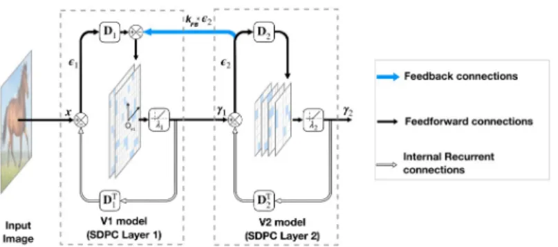
In this paper, we aim at modeling the early visual cortex using a 2-layered version of SDPC (seeFig 1). Consequently, we denote the first and second layer of the SDPC as the V1 and V2 model, respectively. All presented results are obtained with a SDPC network trained with a feedback strength equal to 1 (i.ekFB= 1). Once trained, and when specified, we vary the
feed-back strength to evaluate its effect on the inference process. Note that we have also experi-mented to equate the feedback strength during learning and inference, and the results obtained are extremely similar to those obtained when the feedback strength was set to 1 dur-ing the SDPC traindur-ing. For both databases, all the presented results are obtained on a testdur-ing set that is different from the training set (except when we describe the training in the section
Fig 1. Architecture of a 2-layered SDPC model. In this model,γirepresents the activity of the neural population and
ϵiis the representation error (also called prediction error) at layeri. The synaptic weights of the feedback and
feedforward connection at each layer (DT
i andDirespectively) are reciprocal. The level of sparseness is tuned with the
soft-thresholding parameterλi. The scalarkFBcontrols the strength of the feedback connection represented with a blue
arrow.
entitled ‘SDPC learns localized edge-like RFs in V1 and more specific RFs in V2’). All network parameters and database specifications are listed in the ‘Model and methods’ section.
SDPC learns localized edge-like RFs in V1 and more specific RFs in V2
In this subsection, we present the results of the training of the Sparse Deep Predictive Coding (SDPC) model on both the natural images and the face databases with a feedback strengthkFB
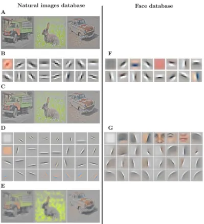
equal to 1 (Fig 2). First-layer Receptive Fields (RFs) exhibit two different types of filters: low-frequency filters, and higher low-frequency filters that are localized, band-pass and similar to Gabor filters (Fig 2B and 2F). The low-frequency filters are mainly encoding for textures and colors whereas the higher frequency ones describe contours. Second layer RFs (Fig 2D and 2G) are built from a linear combination of the first layer RFs. For both databases, the second layer RFs are bigger than those in the first layer (approximately 3 times bigger for both data-bases). We note that for the face database the second layer RFs present curvatures and specific face features, whereas on the natural images database they only exhibit longer oriented edges. This difference is mainly coming from the higher variety of natural images: the identity of
Fig 2. Results of training SDPC on the natural images (left column) and on the face database (right column) with a feedback strength kFB= 1. (A): Randomly selected input images from the natural images database (denotedx in the
text). The two databases are pre-processed with Local Contrast Normalization [40] and whitening. (B) & (F): 16 randomly selected first-layer Receptive Fields (RFs) from the 64 RFs composingDeffT
1 (note thatD effT
1 ¼D
T
1, seeEq 3).
The RFs are ranked by their activation probability in a descending order. The RF size of neurons located on the first layer is 9× 9 px for both databases. (C): Reconstruction of images corresponding to the input images shown in (A) from the representation in the first layer, denotedγeff
1 (note thatγ eff 1 ¼D
T
1γ1, seeEq 18). (D) & (G): 32 sub-sampled
RFs out of 128 RFs composingDeffT
2 (note thatD effT 2 ¼D T 1D T
2, seeEq 3), ranked by their activation probability in
descending order. The size of the RF from neurons located on the second layer is 22× 22 px on the natural images database (D) and 33× 33 px on the face database (G). (E): Reconstruction of images corresponding to the input images shown in (A) from the representation in the second layer, denotedγeff
2 (note thatγ eff 2 ¼D T 1D T 2γ2, seeEq 18). https://doi.org/10.1371/journal.pcbi.1008629.g002
objects, their distances, and their angles of view are more diverse than in the face database. On the contrary, as the face database is composed only of well-calibrated, centered faces, the SDPC model is able to extract curvatures and features that are common to all faces. In particu-lar, we observe on the face database the emergence of face-specific features such as eyes, nose or mouth that are often selected by the model to describe the input (second layer RFs are ranked by their activation probability in descending order inFig 2D and 2G). All the 64 first layer RFs and the 128 second layer RFs learned by the SDPC on both databases are available in the Supporting information section (S1 Figfor natural images andS2 Figfor face database). The first layer reconstruction (Fig 2C) is highly similar to the input image (Fig 2A). In the sec-ond layer reconstructions (Fig 2E), the details like textures and colors are faded and smoothed in favor of more pronounced contours. In particular, the contours of the natural images recon-structed by the second layer of the SDPC are sketched with a few oriented lines.
Effect of the feedback at the neural level
We now vary the strength of the feedback connection to assess its impact on neural representa-tions when an image is presented as a stimulus. The strength of the feedback,kFB, is a scalar
ranging from 0 to 4. WhenkFBis set to 0, the feedback connection is suppressed. In other
words, the neural activity in the first layer is independent of the neural activity in the second layer. Inversely, whenkFB= 4, the feedback signals are strongly amplified such that it reinforces
the interdependence between the neural activities of both layers. As a consequence, varying feedback strength should also affect the activity in the first layer. The objective of this subsec-tion is to study the effect of the feedback on the organizasubsec-tion of V1 neurons (i.e. the first layer of the SDPC).
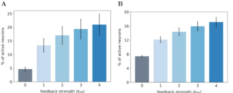
SDPC feedback recruits more neurons in the V1 model. In the first experiment, we
monitor the median number of active neurons in our V1 model when varying the feedback strength on both databases. The medians are computed over 1200 images of natural images database (Fig 3A) and 400 images of the face database (Fig 3B). In this paper, we use the median± median absolute deviation instead of the classical mean ± standard deviation to avoid assuming that samples are normally distributed [41]. For the same reason, all the statisti-cal tests are performed using the Wilcoxon signed-rank test. It will be denotedWT(N = 1200, p < 0.01) when the null hypothesis is rejected. In this notation, N is the number of samples
andp is the corresponding probability value (p-value). In contrast, we will formalize the test
byWT(N = 1200, p = 0.3) when the null hypothesis cannot be rejected.
Fig 3. Percentage of active neurons in the first layer of the SDPC model. (A) On the natural images database. (B) On the face database. We record the percentage of active neurons with a feedback strengthkFBvarying from 0 (no
feedback) to 4 (strong feedback). The height of the bars represent the median percentage of active neurons and the error bars are computed using the median absolute deviation over 1200 and 400 images of the testing set for the natural images and face database, respectively.
For both databases, we observe that the percentage of active neurons increases with the strength of the feedback. In particular, we note a strong increase in the number of activated neurons when we restore the feedback connection (fromkFB= 0 tokFB= 1): +8.7% and +4.7%
for natural images and face databases, respectively. Incrementally amplifying the feedback strength above 1 further increases the number of active neurons in the first layer even if the effect is sublinear. All the increases in the percentage of recruited neurons with the feedback strength are significant as quantified with a Wilcoxon signed-rank test (WT) between all pairs of feedback strength: WT(N = 1200, p < 0.01) for natural images database and WT(N = 400, p < 0.01) for the face database. For each database, we notice that the inter-stimuli variability,
as illustrated by error-bars, is lower when the feedback connection is removed: 0.80% withkFB
= 0 versus 2.55% withkFB= 1 for the natural images database and 0.25% withkFB= 0 versus
0.85% withkFB= 1 for the face database. These results lead us to 2 different conclusions: (1)
The feedback connection tends to recruit more neurons in our model of V1, (2) the feedback signal is dependent of the input stimuli and leads to differentiated effect of the feedback strength.
Interaction map to visualize the neural organization. The V1 activity-map (γ1) being a
high-dimensional tensor, it is a priori difficult to visualize its internal organization. Following our mathematical convention, the activity maps are 3-dimensional tensors of size [nf,wm,hm],
in which the first dimension is describing the feature space (denotedθ), and the 2 last
dimen-sions are related to spatial positions (x and y respectively). One could interpret the activity
maps as a collection ofnf2-dimensional maps describing each feature’s activity in the retinoto-pic space. Said differently, the scalarγ1[j, k, l] is quantifying how strongly correlated is the
fea-ture j (mathematically described byDT
1½j; :; :; :�) with the input image (i.e. x) at the spatial
location of coordinate (k, l). Consequently, we denote θ the space that describes the nffeatures, and we call it the feature space. In practice, we extracted one angle per RF to describe its orien-tation by fitting the first layer features (i.e. those presented inFig 2B and 2F) with Gabor filters [42]. Note that textural and low-frequency filters which are poorly fitted are simply filtered-out (we remove 13 filtered-out of 64 filters). We use the extracted angles to discretized the feature space: y 2 fykgnf
k¼0. Similarly, we describe a space of spatial coordinate (x, y) such thatx 2 ⟦1,
wm⟧ and y 2 ⟦1, hm⟧. One concise way to describe the V1 representation is to formalize it using
the complex number notation denotedγC
1 (seeEq 7).
8y 2 fykgnf
k¼0; 8x 2 ⟦1; wm⟧; 8y 2 ⟦1; hm⟧; γ
C
1½y;x; y� ¼ γ1½ y;x; y� ejy
s:t: j 2 C and j2¼ 1
ð7Þ
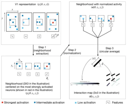
We decompose the computation of the interaction map into 3 steps (seeFig 4for an illus-tration of the computation of the interaction map).
• Step 1 is to extract small neighborhoods around the 10 most strongly activated neurons for each orientation. First, we choose a feature (i.e. an orientation, denotedθc), and we identify the position of the 10 neurons that are the most strongly responsive to the selected orienta-tion. Second, we extract a spatial neighborhoods of size 9× 9 centered on each of these 10 neurons (we thus extract 10 different neighborhoods). We set the size of the neighborhood to be the same than the one of the V2 features (i.e.D2) so that we can capture the feedback
effect coming from V2. At this stage, we have a 10 cropped versions ofγ1which are centered
on neurons strongly responsive to a given orientation. This orientation is called the central preferred orientation (still denotedθc). We use the notation (xc,yc) to describe the spatial coordinates of neurons belonging to the cropped version ofγ1
• Step 2 is to normalize the activity of the neurons in each of 10 cropped versions ofγ1
gener-ated at Step 1. To normalize activity, we use the marginal activity, as defined by the mean neighborhood in a spatially shuffled version of the V1 activity-map. Said differently, the mar-ginal activity, denotedγ1[θ, x*c,y*c], is a spatial average over the activity of neurons that
respond to one given orientationθ. The variables (x*c,y*c) represent the V1-space outside
of this neighborhood. We calla the normalized activity and its computation is defined in
Eq 8.
a½ y; xc;yc� ¼γ1½ y;xc;yc� γ1½ y;x�c;y�c� γ1½ y;x�c;y�c�
ð8Þ Intuitively, for a given (θ, xc,yc),a[θ, xc,yc] is positive if the activity inside the neighborhood
is above the marginal activity and negative in the opposite case.
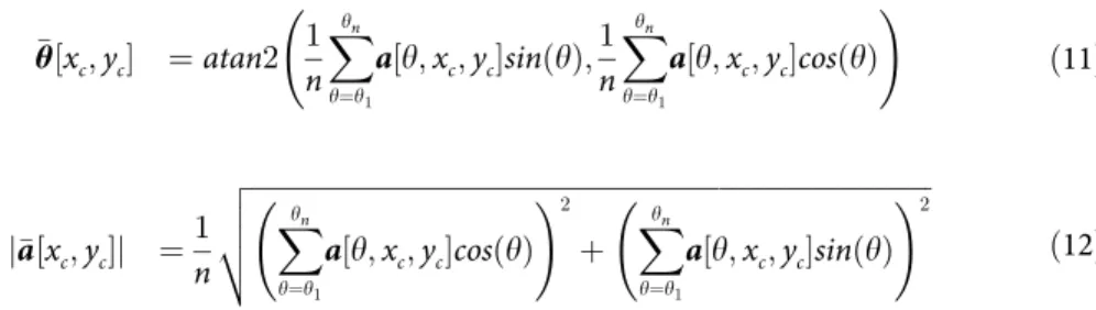
• Step 3 is the actual computation of the interaction map. The interaction map, denoted �a, is computed as the weighted average over all the orientations of the adjusted activity vector (seeEq 9). We denote �θ and j�aj the resulting orientation and activity of the interaction map, respectively (seeEq 10). � a½xc;yc� ¼ 1 n Xyn y¼y1 a½y; xc;yc� �e jy ð9Þ ¼ j�a½xc;yc�j �ej� y½xc;yc� ð10Þ
Fig 4. Illustration of the procedure to generate interaction map. In this illustrative example we consider a V1 representation with only 4 feature maps (represented in the upper-left box). Step 1 is to extract a neighborhood (of size 3x3 in the illustration only) around the most strongly activated neuron (represented with a red square in the
illustration) for a given central preferred orientation (denotedθc). Step 2 is to normalize the neural activity in the
extracted neighborhood using the marginal activity (seeEq 8). Step 3 is to compute the resulting orientation and activity at every position of the neighborhood using a circular mean (see Eqs11and12respectively). To keep a concise figure we have illustrated the computation of the central edge of the interaction map only. For simplification, the illustration shows only 1 neighborhood extraction whereas the interaction maps shown in the paper are computed by averaging neighborhoods centered on the 10 most strongly activated neurons.
We use a circular weighted average to compute the resulting orientation (seeEq 11) and activity (seeEq 12) of the interaction map.
� θ½xc;yc� ¼atan2 1 n Xyn y¼y1 a½y; xc;yc�sinðyÞ; 1 n Xyn y¼y1 a½y; xc;yc�cosðyÞ ! ð11Þ j�a½xc;yc�j ¼ 1 n ffiffiffiffiffiffiffiffiffiffiffiffiffiffiffiffiffiffiffiffiffiffiffiffiffiffiffiffiffiffiffiffiffiffiffiffiffiffiffiffiffiffiffiffiffiffiffiffiffiffiffiffiffiffiffiffiffiffiffiffiffiffiffiffiffiffiffiffiffiffiffiffiffiffiffiffiffiffiffiffiffiffiffiffiffiffiffiffiffiffiffiffiffiffiffiffiffiffiffi Xyn y¼y1 a½y; xc;yc�cosðyÞ !2 þ X yn y¼y1 a½y; xc;yc�sinðyÞ !2 v u u t ð12Þ
Theatan2 operator inEq 11denotes a generalization of the arctangent operator that returns positive angle for counterclockwise angle and opposite for clockwise angle.
At the end of Step 3, we then have generated 10 interaction maps (one for each of the 10 most strongly activated neurons) for a given central preferred orientation. Next, we iterate from Step 1 to Step 3, over 1200 natural images and we average the corresponding interaction maps. At this point, we then have an interaction map for one given central preferred orienta-tion. We then repeat this process for all central preferred orientations and for different feed-back strengths ranging from 0 to 4.
SDPC feedback signals reorganize the interaction map of the V1 model. We investigate
the effect of feedback on the neural organization in our V1 model when the Sparse Deep Pre-dictive Coding (SDPC) is trained on natural images. To conduct such an analysis, we used the concept of interaction map, as introduced previously.
For all feedback strengths and different central preferred orientations, we observe that the interaction maps are highly similar to association fields [19]: most of the orientations of the interaction map are co-linear and/or co-circular to the central preferred orientation (seeFig 5
for one example of this phenomenon andS3 Figfor more examples withkFB= 1). In addition,
interaction maps exhibit a strong activity in the center and towards the end-zone of the central preferred orientation. We define the end-zone as the region covering the axis of the central
Fig 5. Example of a 9× 9 interaction map of a V1 area centered on neurons strongly responding to a central preferred orientation of 30˚. (A) Without feedback. (B) With a feedback strength equal to 1. These interaction maps are obtained when the SDPC is trained on natural images. At each location identified by the coordinates (xc,yc) the
angle is �θ½xc;yc� (seeEq 11) and the color scale is j�a½xc;yc�j (seeEq 12). The color scale being saturated toward both
maximum and minimum activity, all the activities above 0.8 or below 0.3 have the same color, respectively dark or white.
preferred orientation, and the side-zone as the area covering the orthogonal axis of the central preferred orientation. The activity of the interaction map in the side-zone is lower compared to the activity in the end-zone. We notice qualitatively that the orientations of the interaction maps are less co-linear to the central preferred orientation when feedback is suppressed (i.e.
kFB= 0). In other words, when feedback is active, the interaction map looks more organized
compared to the interaction map generated without feedback (seeFig 5for a striking example of this phenomenon).
We next quantify this organizational difference we observed when we turn-on the feedback connection. For a given feedback strengthkFB, we introduce two ratios to assess the change of
the co-linearity (rθco linðkFB)) and co-circularity (rθco cirðkFBÞ) w.r.t. to their respective measure
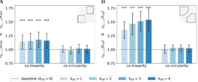
without feedback (see Eqs23and24in sectionModel and methodsfor mathematical details). We report these two ratios for the end-zone (Fig 6A) and the side-zone (Fig 6B). For allkFB > 0, we observe that neurons located in the end-zone and in the side-zone are more co-linear
to the central preferred orientation when the feedback connection is turned on. Indeed, all the bars in the left-block ofFig 6A and 6Bare always above the baseline (as computed as the co-linearity / co-circularity when the feedback is turned off). This increase of co-co-linearity w.r.t. to the baseline is highly significant as measured with the Wilcoxon signed-rank test (WT(N = 51, p < 1e − 3)). We also observe that the increase of co-linearity is more pronounced in the
side-zone (co-linearity bars inFig 6Aexhibit lower values than those inFig 6B). In addition, we note that increasing the feedback strength has a significant effect on the co-linearity in the side-zone as quantified by all pair-wise statistical tests (WT(N = 51, p < 1e − 2)). In contrast,
increasing the feedback strength has no effect on the co-linearity in the end-zone. We observe that the feedback is not changing the co-circularity for neurons located in both the end-zone and the side-zone. Indeed, all the bars in the right-block ofFig 6A and 6Bare near the baseline. Our analysis suggests that the feedback signal tends to modify neural selectivity towards co-lin-earity in both the end-zone and the side-zone.
SDPC feedback signals modulate the activity within the interaction map. To study the
effect of the feedback on the level of activity within the interaction map, we introduce the ratio ra(kFB) between the activity with a certain feedback strength and the activity when the feedback
is suppressed (seeEq 25in sectionModel and methods). Coloring the interaction map using a color scale proportional tora(kFB) allows us to identify which part of the map is more activated
with the feedback. First, we observe qualitatively that the interaction map in the end-zone is more strongly activated when the feedback connection is active. On the contrary, the
side-Fig 6. Relative co-linearity and co-circularity of the V1 interaction map w.r.t. to feedback. (A) In the end-zone. (B) In the side-zone. For each plot, the left and right block of bars represents the relative co-linearity (i.e.rθco linðkFB)) and
co-circularity (i.e.rθco cirðkFB)) with a feedback strength ranging from 1 to 4 w.r.t. their respective value without
feedback (see Eqs23and24). Bars’ heights represent the median over all the orientations, and error bars are computed as the median absolute deviation. The baseline represents co-linearity / co-circularity whenkFB= 0.
zone exhibited weaker activities when feedback is turned on (see Figs7andS4for examples of this phenomenon withkFB= 1). Note also that the activity in the center of the interaction map,
which corresponds to the classical Receptive Field (RF) area, is lowered when feedback is active.
We now generalize, refine and quantify these qualitative observations. We include a third region of interest, the classical RF, to confirm the decreasing activity observed qualitatively at this location. We report the median of the ratiora(kFB) over all central preferred orientations,
for the end-zone, the side-zone, and the classical RF. This analysis is repeated for a feedback strength ranging from 1 to 4 (seeFig 8). We observe an increase of the activity in the end-zone of the interaction map with feedback compared to the end-zone of the interaction without feedback (seeFig 8A). This increase is significant as quantified by all pair-wise statistical Wil-coxon signed-rank tests with the baseline (WT(N = 51, p < 1e − 3)). For larger feedback
strengths, we observe a higher activity in the end-zone which is also significant (all pair-wise statistical tests between all feedback strengths (WT(N = 51, p < 0.01)). For example, in the
end-zone, the median activity over all the central preferred orientations is 16% and 25% higher with a respective feedback strength of 1 and 4 compared to the median when feedback is sup-pressed. This suggests that the feedback signals excite neurons in the end-zone of the interac-tion map. In contrast, we observe a slight decrease of activity in the side-zone of the
interaction map with feedback active compared to when feedback is suppressed (seeFig 8B). The decrease compared to the baseline is significant forkFB= 1 andkFB= 2 (WT(N = 51, p < 1e − 2)). For higher feedback strength, the lowered activity in the side zone becomes less
significant. The activity in the classical RF exhibits a significant decrease compared to the base-line (WT(N = 51, p < 1e − 3)). In addition, the larger the feedback strength, the weaker the
activity in the center of the interaction map (WT(N = 51, p < 1e − 2)). For example, we report
a change in the decrease from−28% for kFB= 1 to−34% for kFB= 4 compared to the activity in
the center of the interaction map without feedback (seeFig 8C).
Fig 7. Example of a 9× 9 interaction map of a V1 area centered on neurons strongly responding to a central preferred orientation of 45˚, and colored with the relative response w.r.t. no feedback. The feedback strength is set to 1 and the SDPC is trained on natural images. At each location identified by the coordinates (xc,yc) the angle is
�
θ½xc;yc� (seeEq 11) and the color scale is proportional tora(kFB) (seeEq 25). The color scale being saturated toward
both maximum and minimum activity, all the activities above 1.3 or below 0.5 have the same color, respectively dark green or purple.
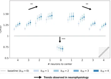
We report the spatial profile of the median activity along the axis of the central preferred orientation (seeFig 9). For all distances from the center, the activity along the central preferred orientation axis of interaction map is significantly higher than the activity without feedback (all pair-wise statistical tests with the baseline: WT(N = 51, p < 1e − 2)). The only exception is
in the classical RF of the interaction map, where the activity is weaker when feedback is active (see alsoFig 8C). This inhibition in the classical RF of the map compared to the baseline is sig-nificant as quantified with pair-wise statistical tests (WT(N = 51, p < 1e − 3)). Even if activities
forkFB6¼ 0 along the central preferred orientation axis are always higher than the activity with kFB= 0, they tend to decrease with distance to the center (pair-wise statistical test for different
locations: WT(N = 51, p < 1e − 2)). Especially, for kFB= 4, the neurons located just near the
center exhibit a response +36% higher than the same neurons without feedback. With the
Fig 8. Relative response of V1 interaction map w.r.t. no feedback for all central preferred orientations. (A) In the end-zone. (B) In the side-zone. (C) In the center (i.e. classical RF). Bars’ height represent the median over all the central preferred orientations, and error bars are computed as the median absolute deviation. The computation of the relative response, denotedra(kFB), is detailed inEq 25. The baseline represents the relative response without feedback.
Black arrows represent the trends observed in neurophysiology (see section ‘Comparing SDPC results with neurophysiology’ for more details).
https://doi.org/10.1371/journal.pcbi.1008629.g008
Fig 9. Relative response w.r.t. no feedback along the axis of the central preferred orientation of V1 interaction map. Each point represents the median over all the orientations, and error bars are computed as the median absolute deviation. The x-axis represents the distance, in number of neurons, to the center of the interaction map. The computation of the relative response, denotedra(kFB), is detailed inEq 25. The baseline represents the relative response
without feedback. Black arrows represent the trends observed in neurophysiology (see section ‘Comparing SDPC results with neurophysiology’ for more details).
same feedback strength, this increase of activity w.r.t to no feedback is reduced to 15% when the neurons are located 4 neurons away from the center. At a given position different from the center, increasing the feedback strength significantly increases the activity as quantified by all pair-wise statistical test (WT(N = 51, p < 1e − 2)).
Our results exhibit three different kinds of modulations in the interaction map due to feed-back signals. First, the activity in the classical RF of the map is reduced with the feedfeed-back. Sec-ond, the activity in the end-zone, and more specifically along the axis of the central preferred orientation is increased with the feedback. Third, the activity in the side-zone is reduced with the feedback.
Effect of the feedback at the representational level
After investigating the effect of feedback at the lowest level of neural organization, we now explore its functional and higher-level aspects. In particular, this subsection is dealing with the denoising ability of the feedback signal.
Denoising abilities emerge from the feedback signals of the SDPC. To evaluate the
denoising ability of the feedback connection, we feed the Sparse Deep Predictive Coding (SDPC) model with increasingly more noisy images extracted from the natural images and the face databases. Then, we compare the resulting representations (γeff
i ) with the original
(non-degraded) image. To do this comparison, we conduct two types of experiments: a qualitative experiment that visually displays what has been represented by the model (see Figs10Aand
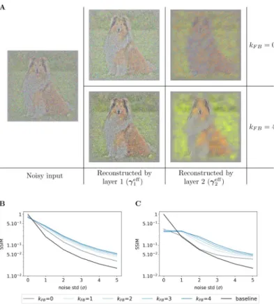
S5A), and a quantitative experiment measuring the similarity between representations of noisy and original images (seeFig 10B and 10Con natural images andFig 11A and 11Bon face data-base). These two experiments are repeated for a noise level (σ) ranging from 0 to 5 and a
feed-back strength (kFB) varying from 0 to 4. The similarity between images is computed using the
median structural similarity index [43] over 1200 and 400 images for the natural images and face database, respectively. The structural similarity index varies from 0 to 1 such that the more similar the images, the closer the index is to 1. For comparison, we include a baseline (see the black curves in Figs10and11) which is computed as the structural similarity index between original and noisy images for different levels of noise. It is important to note that this experiment has been conducted without re-training the SDPC. Therefore, the network is trained on non-degraded natural images and has not been explicitly asked to denoise degraded images.
We first observe that whatever the feedback strength, the first layer representations of the original image (first row, column 2 to 6 inS5A Fig) are relatively similar to the input image itself. This observation is supported by a structural similarity index close to 0.9 for all feedback strengths (σ = 0 inFig 10Bfor natural images andFig 11Afor faces). On the contrary, second layer representations look more sketchy and exhibit fewer details than the image they repre-sent (first row, column 7 to 11 inS5A Fig). This is also quantitatively backed by a structural similarity index fluctuating around 0.4 for the natural images database (σ = 0 inFig 10C) and 0.6 for the face database (σ = 0 inFig 11B). Interestingly, when input images are corrupted with noise (i.e. whenσ � 1), and whatever the feedback strength, first layer representations
systematically exhibit higher structural similarity index than the baseline (Fig 10Bfor natural images andFig 11Afor faces). This denoising ability of the SDPC, even without feedback is significant as reported by the pair-wise Wilcoxon signed-rank tests with the baseline for both databases (WT(N = 1200, p < 1e − 2) for natural images database, and WT(N = 400, p < 1e
− 2) for the face database). More importantly, the higher the feedback strength, the higher the similarity index. In particular, on the natural images database, when the input is highly degraded by noise (σ = 5), the similarity is 0.02 for the baseline, 0.03 for kFB= 0, 0.05 for
Fig 10. Effect of the feedback strength on noisy images from natural images database. (A) In the left column, one image is corrupted by Gaussian noise of mean 0 and a standard deviation of 2 (σ). The central column exhibits the representations made by the first layer (γeff
1), and the right-hand column the representations made by the second layer
(γeff
2). Within each of these blocks, the feedback strength (kFB) is equal to 0 in the top line and 4 in the bottom line. (B)
We plot the structural similarity index (higher is better) between original images and their representation by the first layer of the SDPC. (C) We plot the structural similarity index between original images and their representation by the second layer of the SDPC. All curves represent the median structural similarity index over 1200 samples of the testing set and present a logarithmic scale on the y-axis. The color code corresponds to the feedback strength, from grey for kFB= 0 to darker blue for higher feedback strength. The black line is the baseline, it is the structural similarity index
between the noisy and original input images.
https://doi.org/10.1371/journal.pcbi.1008629.g010
Fig 11. Effect of the feedback strength on noisy images from face database. This figure description is similar to the description of theFig 10B and 10C. For the face database, all presented curves represent the median structural similarity index over 400 samples of the testing set.
kFB= 1 and 0.06 forkFB= 4 (seeFig 10B). This improvement of the denoising ability with
higher feedback strength whenσ = 5 is also significant as quantified by the pair-wise statistical
tests between all feedback strengths (WT(N = 1200, p < 1e − 2)). The inter-image variability of
the structural similarity of first layer representation as quantified by the median absolute devi-ation is low compared to the median similarity on the natural images database (seeS5D Fig). In the face database, for a highly degraded input (σ = 5), the structural similarity index is 0.01
for the baseline, 0.03 forkFB= 0, 0.05 forkFB= 1 and 0.07 forkFB= 4. On the face database, the
increases of the first layer similarity with the feedback strength when inputs are highly degraded (σ = 5) are significative as measured by all the pair-wise statistical tests between all
feedback strengths (WT(N = 400, p < 1e − 2)). Inter-image variability of the similarity of the
first layer representation is also lower than the corresponding median on the face database (see
S6C Fig). Our analysis suggests that the feedback connection in the Predictive Coding (PC) framework (i.e. whenkFB> 0) allows the first layer of the network to better denoise degraded
images. It is interesting to mention again that this property is emergent as the network has never been explicitly trained to denoise degraded images.
Effect of sparsity on denoising. We have seen in the previous subsection that the
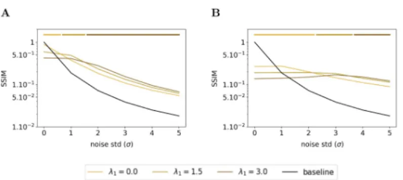
feed-back connection exhibited an emergent denoising ability. In this subsection, we wonder what is the effect of the sparsity on the denoising ability of the Sparse Deep Predictive Coding (SDPC). To answer this question, we feed the SDPC with increasingly blurred images, we vary the level of the sparsity in the first layer during inference (i.e.λ1) and we assess its impact on
the reconstruction quality using the structural similarity index. Figs12and13show the evolu-tion of the similarity on the natural images and face databases and for 3 different levels of spar-sity on the first layer: no sparspar-sity at all (i.e.λ1= 0), intermediate sparsity (i.e.λ1= 1.5), and high
sparsity (i.e.λ1= 3.0). We observe that high sparsity levels are beneficial for better
reconstruc-tion quality of the first layer when the input images are strongly degraded (see dark brown curves in Figs12Aand13A). In contrast, when input images are not degraded at all (i.e.σ = 0),
the lower the first layer sparsity the better the reconstruction quality (see light brown curves on Figs12Aand13A). In addition, we observe a similar phenomenon for the second layer of the SDPC (see Figs12Band13B). Our analysis suggests that sparsity is playing a crucial role when it comes to denoise strongly degraded input images.
In this section, we conducted a qualitative and quantitative analysis of the denoising ability of Sparse Deep Predictive Coding (SDPC) model. Our results suggest that not only the feed-back connection but also the sparse representation allows the SDPC to better recover images
Fig 12. Effect of the first layer sparsity on noisy images from natural images database with kFB= 4. (A) Structural
similarity index between original images and their representation by the first layer of the SDPC. (B) Structural similarity index between original images and their representation by the second layer of the SDPC. Top lines represent the sparsity levels that maximize the similarity for different levels of degradation. All presented curves represent the median structural similarity index over 1200 samples of the testing set.
degraded with noise. Therefore, the emergent denoising ability of the proposed model is directly deriving from the combination of the 2 components of the SDPC that are Sparse Cod-ing and Predictive CodCod-ing. The superior denoisCod-ing capacity of the 2ndlayer of the SDPC sug-gests that the network is able to disentangle informative features from noisy background. Such a disentangling mechanism might help the network to better recognize object when the input is corrupted.
Discussion
Herein, we have conducted computational experiments on a 2-layered Sparse Deep Predictive Coding (SDPC) model. The SDPC leverages feedforward and feedback connections into a model combining Sparse Coding (SC) and Predictive Coding (PC). As such, the SDPC learns the causes (i.e. the features) and infers the hidden states (i.e. the activity maps) that best describe the hierarchical generative model giving rise to the visual stimulus (seeFig 14for an illustration of this hierarchical model andEq 1for its mathematical description).
Fig 13. Effect of the first layer sparsity on noisy images from face database with kFB= 4. This figure description is
similar to the description of theFig 12. For the face database, all presented curves represent the median structural similarity index over 400 samples of the testing set.
https://doi.org/10.1371/journal.pcbi.1008629.g013
Fig 14. Illustration of the hierarchical generative model learned by the SDPC model on the face database. The deepest prediction (first row) is viewed as the sum of the features prediction (the second row). These feature predictions are computed as the convolution between one channel ofγ2and the corresponding features inD2.
Similarly, the eyes can be decomposed usingγ1andD1(the third row).
We use this model of the early visual cortex to assess the effect of the early feedback connec-tion (i.e feedback from V2 to V1) through different levels of analysis. At the neural level, we have shown that feedback connections tend to recruit more neurons in the first layer of the SDPC. We have introduced the concept of interaction maps to describe the neural organiza-tion in our V1-model. Interestingly, the interacorganiza-tion maps generated when natural images are presented to the model are very similar to biologically observed association fields. In addition, interaction maps allow us to describe the neural reorganization due to feedback signals. In particular, we have observed that feedback signals align neurons co-linearly to the central pre-ferred orientation. At the activity level, we observe three different kinds of feedback modula-tory effects. First, the activity in the classical Receptive Field (RF) is decreased. Second, the activity in the end-zone of the extra-classical RF and more specifically along the axis of the cen-tral preferred orientation is increased. Third, the activity in the side-zone of the extra-classical RF is reduced. At the representational level, we have investigated the role of feedback signals when input images are degraded using Gaussian noise. We have demonstrated that higher feedback strengths allow better denoising ability. We have also shown that sparsity plays a cru-cial role to recover degraded images. In this section, we link our model with the original PC model [29] and we interpret our computational findings in light of current neuroscientific knowledge.
SDPC extends Rao & Ballard’s PC model
The Sparse Deep Predictive Coding (SDPC) model is directly inspired by the Predictive Cod-ing (PC) model proposed by Rao & Ballard [29] and extends it to a scale that is more realistic for cortical processing in the visual cortex. The original PC model had few dozens of neurons (20 in the first layer and 32 in the second one), linked with fully-connected synapses and trained on patches extracted from 5 natural images. In this work, the SDPC leverages hundreds of thousands of neurons (� 5× 10⁵neurons in the first layer, � 8× 10⁵neurons in the second layer for the network trained on natural images) and convolutional synaptic weights trained on thousands of natural images. In terms of analysis, the interaction maps we introduced con-firm and extend the results from Rao & Ballard. Our model also described the end-stopping effects inside the classical Receptive Field (RF): we observed a strongly decreased activity in the classical RF for extended contours when the feedback connection was activated (see Fig 5 from [29] and see Figs8Cand9). Last but not least, the convolutional framework of the SDPC allows us to extend the Rao & Ballard findings beyond the classical RFs and to observe that feedback signals play a role in the extra-classical RF. It tends to reinforce neural activity along the preferred orientation axis (see Figs9and7) and to reshape neural selectivities to better reflect association fields.
SDPC learns cortex-like RFs while performing neuro-plausible
computation
The Sparse Deep Predictive Coding (SDPC) model satisfies some of the computational con-straints that are thought to occur in the brain, notably local computations [44]. The locality of the computation is ensured byEq 5: the new state of a neural population (whose activity is rep-resented byγtþ1
i ) only depends on its previous state (γ t
i), the state of adjacent layers (γ t i 1and
γt
iþ1) and the associated synaptic weights (DiandDi+1). In the SDPC we have used the
convolu-tional framework to enforce a retinotopic organization of the activity map. The convoluconvolu-tional operator suggests that features are shared at every position of the activity map. This assump-tion has the advantage to model the posiassump-tion invariance of RFs observed in the brain. Never-theless, the weight-sharing mechanism is far from being bio-plausible. Interestingly, recent
studies have shown that imposing local RFs to fully connected synapses allows to mimic con-volutional features without enforcing the weight-sharing mechanism [45]. Therefore, it sug-gests that convolution-like operations might be implemented in the brain in the form of locally-connected synapses. All these neuro-plausible constraints we have included in the SDPC makes it unique compared to frameworks like feedforward neural networks or auto-encoders. These networks are trained using a global loss function minimized through back-propagation and do not leverage top-down signals during the inference process. Not only the processing but also the result of the training exhibits tight connections with neuroscience. The first-layer Receptive Fields (RFs) (Fig 2Bfor the natural images database andFig 2Ffor the face database) are similar to the V1 simple-cells RFs, which are oriented Gabor-like filters [46,
47]. Olshausen & Field have already demonstrated, in a shallow network, that oriented Gabor-like filters emerge from sparse coding strategies [25], but to the best of our knowledge, this is the first time that such filters are exhibited in a 2-layers network combining neuro-plausible computations with Predictive Coding and Sparse Coding (in [29], Rao & Ballard exhibited only first layer filters on their model constrained with a sparse prior). This architecture allows us to observe an increase in the specificity of the neuron’s RFs with the depth of the network. This observation is even more striking when the SDPC is trained on the face database, which presents less variability compared to the natural images database. On face images, second layer RFs exhibit features that are highly specific to faces (eyes, mouth, eyebrows, contours of the face). Interestingly, it was demonstrated with neurophysiological experiments that neurons located in deeper regions of the central visual stream are also sensitive to that particular face features [48,49].
Comparing SDPC results with neurophysiology
At the electrophysiological level, it has been demonstrated that as early as in the V1 area, feed-back connections from V2 or V4 could either facilitate [12] or suppress [16] lateral interac-tions. These modulations help V1 neurons to integrate contextual information from a larger part of the visual field and play a causal role in increasing and decreasing activity for neurons encoding for the contour and the background, respectively [18,50,51]. The SDPC model behaves similarly: i)Fig 8Ais showing a feedback-dependent increase of activity for neurons located in the end-zone (i.e. in the direction of the contour) and ii)Fig 8Bexhibits a feedback-dependent decrease activity of neurons located in the side-zone (i.e. in the direction of the background). As mentioned in the previous subsection, the SDPC is also consistent with the increase of end-stopping effect related to the increase of the feedback strength. In electrophysi-ology these phenomenons has been observed in monkeys using attentional modulations (that we will interpret as a modulation of the feedback strength) [52] or by cooling-down areas located after V1 to remove the feedback signals [17]. Moreover, it has been demonstrated that the neural excitation due to feedback signal from V4 to V1 on neurons located on contours was strongly dependent on the length of the contours [18]. An extended contour triggered smaller extra-feedback signals compared to shorter contours (see Fig 2A in [18]). This electrophysiological observation is in line with the SDPC results shown inFig 9: neurons located along the axis of the contour but far away from the classical Receptive Field (RFs) are less strongly excited than those closer to the classical RF.
Functional interpretation of the observed V1 interaction maps
It was assumed that association fields were represented in V1 to perform such a contour inte-gration [21]. Interestingly, SDPC first-layer interaction maps exhibit a co-linear and co-circu-lar neural organization very simico-circu-lar to association fields even without feedback (seeFig 5). We