History of Numerical Tables in Sanskrit Sources

HAL Id: halshs-01006137

https://halshs.archives-ouvertes.fr/halshs-01006137

Submitted on 13 Jun 2014

HAL is a multi-disciplinary open access

archive for the deposit and dissemination of

sci-entific research documents, whether they are

pub-lished or not. The documents may come from

teaching and research institutions in France or

abroad, or from public or private research centers.

L’archive ouverte pluridisciplinaire HAL, est

destinée au dépôt et à la diffusion de documents

scientifiques de niveau recherche, publiés ou non,

émanant des établissements d’enseignement et de

recherche français ou étrangers, des laboratoires

publics ou privés.

History of Numerical Tables in Sanskrit Sources

Agathe Keller, Koolakodlu Mahesh, Clemency Montelle

To cite this version:

Agathe Keller, Koolakodlu Mahesh, Clemency Montelle. History of Numerical Tables in Sanskrit

Sources. Tournes, Dominique. History of Numerical Tables, Springer, In press, WSAWM.

�halshs-01006137�

Numerical Tables in Sanskrit Sources

Agathe Keller, Mahesh K., Clemency Montelle

March 25, 2014

Abstract

Sanskrit sources offer a wide variety of numerical tables, most of which remain little studied. Tabular information can be found encoded in verse, woven into prose, sometimes arranged in aligned grids of rows and columns but also in other, less standard patterns. We will consider a large range of topics from mathematical (gaṇita) and astral science (jyoṭiṣa) sources. Among the mathematical sources, we will explore sine tables, units of measurement, combinatorial relations, as well as the related ephemeral arrays used in computation. Among the latter, we will investigate astronomical tables of various sorts, including aligned tables, lists of aphorisms which code numbers, and almanacs. In all the cases, we will show the ways in which the variety and complexity of the material challenges more standard characterizations of numerical tables in other contexts. Further, how numerical tables relate to algorithms, in their content, execution, and presentation, will be advanced, in a way which will be a unifying feature of our coverage. Indeed, the interconnection between numerical table and algorithm has profound implications for other contexts presented in this book.

Contents

1 Introduction 3

2 Numerical tables in Sanskrit mathematical sources 4

2.1 Ephemeral computational arrays . . . 5

2.1.1 Decimal place-value notation . . . 5

2.1.2 Operations . . . 7

2.1.3 Other algorithms . . . 9

2.2 Non-ephemeral numerical arrays . . . 10

2.2.1 Vernacular tables for elementary operations . . . 10

2.2.2 Combinatorial tables . . . 12

2.2.3 Magic squares . . . 19

2.3 Textual tables in mathematics . . . 24

2.3.1 Tables for elementary operations in words . . . 24

2.3.2 units of measurement . . . 25

2.3.3 Sines . . . 27

2.3.4 A list of solutions of linear indeterminate equations . . . 28

3 Numerical Tables in Astral sources in Sanskrit 29 3.1 Tabulating data in rows and columns . . . 29

3.2 The Brahmatulyasāraṇī: Reckoning solar declination in tabular and non-tabular sources . . . 33

3.3 Three types of planetary tables . . . 38

3.4 South Indian Astronomical Tables . . . 44

1 Introduction

The Indian subcontinent testifies to a wide variety of numerical tables. Our own rough estimate suggests that the extent of the corpus may go into the hundreds of thousands, stretching over almost two millennia. Numerical tables can be found in a variety of media: on instruments, inscriptions, and manuscripts. They can be found in numerous textual genres, with a variety of applications. For instance, poetic calligrams (citrakāvya), magical tabular diagrams (cakras) used to ensure victory in battle [Sarma 2012 c, Sarma 2012 b], musical tables for enumerating the number of talas in a given rāga [Patte 2012], [Sridhara Srinivas 2012] or the array of the numbers of long and short syllables in a verse [vanNooten 1993], [Sarma 2003], [Plofker 2009]. Some works consist of tables AS text, while others consist entirely of tables. Tabular information can be found encoded in verse, woven into prose, sometimes arranged in aligned grids of rows and columns but also in other, less standard patterns. This variety and complexity challenges most standard characterizations of numerical tables.

In Sanskrit astral and mathematical sources, different kinds of objects have been labeled as “tables” by historians of mathematics. These include: verbally encoded, sometimes versified, lists of precomputed numerical data (Sines, for example), row and column astronomical tables-texts; definitions of and conversions between units of measurement; ephemeral computational arrays; calendars and almanacs; permutation and combinatorial devices; and divinatory and auspicious arrangements of numbers and objects, to name but a few.

In the face of such diversity, rather than adhere to a narrow definition of a table (e.g. an object displaying tabular information in an aligned grid of rows and columns), we embrace all sorts of tabular layouts in their broadest sense as key and relevant to the study at hand. Throughout this survey we will examine how these objects were thought of by the actors who created or used them, and how historians have understood the objects in relation to tables.

Our account has two main themes:

• Investigating the numerous ways of storing tabulated numerical data • Examining the interrelationships between numerical tables and algorithms

It is not always easy to SKETCH OUT/DESCRIBE the broader context in which the astral sciences

(jyoti-ṣa) and mathematics (gaṇita) were practiced and developed in India. One of the purposes of the astral sciences

appears to have been the construction yearly almanacs (pañcāṅgas). Many of the numerical tables that were produced and used can thus be contextualized to some extent as directed towards this end.

As early as the 6th century CE three distinct elements can be identified in the practice of mathematical and astral science which are relevant to the study at hand:

1. Ephemeral numerical arrays used for computations; 2. Sometimes abstruce rules (sūtras) for algorithms;

3. Mnemonic strings of numbers for storage (parameters, sine differences, etc.)

By the twelfth century a conceptual shift appeared in the way algorithms and data were related, which took different forms in North and South India. Data resulting from mathematical procedures took on a new

importance, pre-computed numerical values were integrated into THE EXECUTION OF algorithms, taking the form of increasingly large mnemonic lists or arrays, and largely autonomous compositions of table-texts emerged. By the seventeenth century, there were a large number of such numerical table-texts, and their use was widespread.

Features of the various ways in which early practitioners gave expression to tabular numerical material, both in verse as well as in accompanying prose commentaries are explored in section 2. The emergence of such texts, largely concentrated in North India, and their features will be examined in sections 3.1, 3.3 and the flourishing of contrasting strands of encoded numerical data in South India will be explored in section 3.4.

This survey is largely restricted to mathematical and astronomical numerical tables in Sanskrit textual sources, dating roughly from the beginning of the Common Era to the seventeenth century. Therefore, many known numerical tables from the subcontinent have been omitted. For instance, relevant sources written in vernacular Indian languages, such as Prakṛit, Malayalam, or Persian have been given minimum coverage despite their abundance. Similarly, the graphical tables on Indian astrolabes [Sarma 2012 a] and the numerical tables that circulated in the Indian subcontinent as it progressively industrialized in the 19th century, and so forth, will not be examined here.

The large corpus of Sanskrit numerical tables in the mathematical and astronomical sciences in Sanskrit has been investigated by a number of scholars, but much work remains to be done. David Pingree has produced a census of manuscripts which contains many expmples of numerical tables [Pingree CESS]. He has also produced specific catalogues of tables, most notably in American and British collections [Pingree 1968], [Pingree SATE]. He has also studied the range and scope of numerical tables [Pingree 1970], [Pingree 1981, 41-51]. Specific tables have also been analyzed [Yano 1977], [Kusuba 1994], [Ikeyama Plofker 2001], [Venketeswara Joshi Ramasubramaniam 2009], IJHS forthcoming.

2 Numerical tables in Sanskrit mathematical sources

From the 5th century onwards numerical tables in mathematics (gaṇita) took two different but related forms: tabular information expressed in words, although not in COMMON language (THIS IS SUPPOSE TO BE A SYNTHETIC REFERENCE TO SYLABICAL CODES WITH NO MEANING, VERSES MADE OF COM-POUNDED NAMES OF DIGITS OR TEXTS WITH DOUBLE MEANINGS: A PROVERB CODING A LIST OF NUMBERS) and ephemeral numerical arrays.

The Sanskrit scholarly tradition in the first and second millennium mainly copied and transmitted UNDER THE NAME gaṇita texts dealing with mathematical astronomy. However, gaṇita could also feature topics distinct from astral lore [Pingree 1981],[Keller 2007]. In this section NUMERICAL TABLES RELEVANT TO NON ASTRAL MATHEMEMATICS will be examined before turning to numerical tables which have more direct astronomical applications.

2.1 Ephemeral computational arrays

One of the distinct features of Sanskrit mathematical commentaries is the glimpse they give us of a working surface onto which numerical arrays can be drawn.

Indeed, while treatises give versified mathematical rules and sometimes list associated examples (uddeśaka,

udahāraṇa), the commentaries, after glossing the rule in general terms always solve several problems following

a more or less standard structure: the statement of the problem, often versified as a riddle, is followed by a setting (nyāsa, sthāpana) of the data given in the problem, and its resolution (karaṇa). This setting opens a door in the text onto a working surface on which computations were executed and diagrams drawn, giving us a glimpse of how algorithms were carried out in practice. Computational arrays often appear in these settings, emerging in manuscripts, sometimes without being referred to in words. These computational arrays have tabular frameworks— rows and columns — in which numbers are written down and manipulated. They are ephemeral, because they are used transitionally while executing an operation or an algorithm, disappearing at the end of the execution. Key to the array as a computational tool is the use of the layout’s graphical characteristics independently from its mathematical properties. The extent to which transitional arrays also use numerical tables’ other advantages, such as storing values and expressing two variables functions will also be examined here.

2.1.1 Decimal place-value notation

Decimal place-value notation appears in Sanskrit mathematical sources from around the 5th century CE. A stan-dard explanation of its world-wide spread underlines how place-value creates a computational grid: operations using it can be executed more or less mechanically; numerical significance can be ascertained when needed by analyzing the relative positions of the digits.

Are such resources used in Sanskrit mathematical texts? Do the authors provide us with insights of how they understood decimal place-value notation, and its “tabular” characteristics?

One of the first such definitions is found in the mathematical chapter of the Āryabhaṭīya (499) of Āryabhaṭa and runs as follows [Shukla 1976]1_:

Ab.2.2. One and ten and a hundred, and one thousand, now ten thousand and a hundred thousand, in the same way a million|

Ten million, a hundred million, and a thousand million. A position should be ten times the ⟨previous⟩ position∥

Structurally, the definition of decimal place-value notation in Sanskrit sources remained unchanged from the 5th to at least the 12th century, always listing increasing powers of ten, followed by an algorithm concerning positions (sthāna).

The authors of these definitions do seem to have considered decimal place-value notation as an ordered row whose cells represented increasing powers of ten in which digits could be written to form a number. Indeed,

1_{ekaṃ ca daśa ca śataṃ ca sahasraṃ tv ayutaniyute tathā prayutam|} koṭyarbudaṃ ca vṛndaṃ sthānāt sthānaṃ daśaguṇaṃ syāt∥

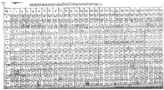
the order of such a row is what links both elements of what are seemingly two separate parts of the rule: The sequence of powers of ten appears as a first clause. The way this sequence is ordered is revealed through an algorithm in the second clause. Such a row is embodied in Bhāskara’s 7th century commentary, the earliest handed down to us, on the above definition by Āryabhaṭa. This commentary ends with the following statement [Shukla 1976]2_:

And the setting of positions is: ° ° ° ° ° ° ° ° °

Figure 1: The positions of decimal place-value as a row of small circles

In Figure 2.1.1, this row is displayed as it can be found both in Shukla’s edition of the text [Shukla 1976] and in the Burnell 517 manuscript, belonging to the British Library, which probably dates from the 19th century3_{. The order of the list of powers of ten in the definition goes from smaller to higher powers of ten.}

Indeed, commentaries testify to the fact that positions were counted from right to left, the first being for the lowest power of ten. THE EVIDENCE FOR THIS ORDER IS PARTICULARLY STRIKING IN THE WAY A LARGE NUMBER IS USUALLY STATED: ITS DIGITS ARE COMPOUNDED WITH AN ENUMERATION IN WORDS IN INCREASING POWERS OF TENS AND THEN THE NUMERAL IS WRITTEN AS WE ARE USED TO, WITH DECREASING POWERS OF TEN, FROM LEFT TO RIGHT4_{. FOR INSTANCE, IF}

WE CONSIDER Bhāskarācārya’S (B.1114) LIST OF DIFFERENCES IN SOLAR DECLINATION EVOKED IN SECTION 3.2, WHICH STARTS WITH THE VALUE 362: IT IS STATED IN WORDS THROUGH A COMPOUND WHICH READS FROM LEFT TO RIGHT “TWO-SIX-THREE” (YAMĀṄGARĀMA). SUCH A COMPOUND REFERS TO A NUMERAL IN DECIMAL PLACE-VALUE NOTATION, BUT PROVIDES THE DIGITS IN INCREASING POWERS OF TEN. HOWEVER THE NOTED NUMERAL HAS DIGITS WHICH ARE FROM LEFT TO RIGHT IN DECREASING POWERS OF TEN: 3-6-2. TEXTS OFTEN CONTAIN BOTH, THE COMPOUND AND THE NUMERAL. This double statement highlights THAT the expression of VALUES IN WORDS HAD TO BE ARTICULATED WITH numerical notations5_{. The order}

2_{nyāsaś ca}

sthānānām-3_{Note that since the manuscript is very recent, it is the existence of a text preceding such a layout that suggests that it appeared} within the text of Bhāskara’s commentary. ‘However, since this sentence cannot be found in all the manuscript versions of Bhāskara’s commentary, only a new critical edition, or the finding of a new manuscript version of the work would ascertain the existence of this sentence and the layout that went with it.

4_{In other words, the digits are enumerated in the direction of reading and writing, which is from left to right (most classical Sanskrit} scripts were written in that direction), but seemed to be noted from right to left. This is a well-known, much discussed fact -see [Salomon 1998]- whose historiographical debates are evoked in [Keller 2011]. Note that the right to left movement has little been taken in account when attempting to reconstruct algorithm’s executions.

5_{Further, in this case the digits are named with the Sanskrit “word numeral” (bhuta-saṅkhyā) system, rather than with simple names} for digits.

of digits is central to this articulation. Decimal place-value notation was also useful for storing numbers: it is commonplace in astronomical texts for the textual enunciation of a number to be repeated with its decimal place-value notation to ensure that large numbers are not corrupted.

As decimal place-value notation is thus standardly conceived as a notation for numbers using an ordered row of digits, we could expect that operations on values written in this notation would also use this layout, expanding it into an ephemeral computational array. As we will see, the existing Sanskrit sources show a much more complex state of affairs.

2.1.2 Operations

Many definitions were given to mathematics (gaṇita) by Sanskrit authors. Such definitions standardly consisted in listing operations (parikarman) and specific topics, “practices” (vyavahāra), whose number and contents could change from author to author [Datta Singh 1935], [Keller 2007], [Plofker 2009]. Operations consisted of addition, subtraction, multiplication, division, square, square root, cube and cube root (usually in that order, but some authors put multiplication first) followed sometimes with rules on different classes of fractions, and rules for proportions.

Very few texts detail how the first four operations were executed. When this is the case they are allusive and require commentaries, which for the most part have been transmitted in single recent fragmentary manuscripts. Furthermore, not all these commentaries have been closely studied or properly edited, so that further scholarship in the following years will no doubt clear some of the questions raised here. In most cases, operations linking single digits (that is 2 × 9 or 7 − 4) are assumed to be known. To the best of our knowledge no documents in Sanskrit sources provide tables of elementary operations; some can be found in fairly recent vernacular language manuscripts[Sarma 1997]6_{. Rules for operations implicitly concern those on larger numbers, that is written}

with more than one digit. The execution of such operations did not always use place-value grids. Concerning multiplication for instance, authors evoke several methods with specific names such as “zigzag” (go-mutrikā), “as it stands” (tat-stha), “portions” (khaṇḍa), etc. These methods change from author to author and seem to have evolved over time7_{. Only the multiplication called “door-junction” (kavāṭa-sandhi or kapāṭa-sandhi) uses}

the columns defined by the positions of decimal place-value notation in all cases.

Other operations have rules which are more systematically linked to how numbers are written. This is the case of squaring, cubing and extracting square and cube roots. Thus, for example, to extract square roots, the positions in which the digits of the numeral whose square root is to be extracted are counted from right to left, and numbered according to their order: the first position, is position 1, the second position, position 2, etc. Such positions are then singled out according to whether they are even or odd. Position 2, is an even position, position 3, an odd position, and so forth. The positions characterized in this way only use the fact that the layout is a row, not that powers of ten are denoted by these positions. Of course, a correspondence can be made:

6_{These will be studied in the next sub-section as well as in the section studying verbal mathematical tables in Sanskrit.}

7_{A thorough study of Brahmagupta’s, Mahāvīra’s and Śrīdhara’s different multiplication methods is to be published by A. Keller and} C. Singh in a forthcoming book on Cultures of Computation and Quantification. A draft can be found here: (hal shs forthcoming)***. See also Keller forthcoming in French.

odd positions correspond to even powers of ten, that is square powers of ten, which is precisely the mathematical property on which the square root extraction is grounded. But to carry out the process this fact is incidental. Here then the authors consider place-value as a formal graphical device creating a grid for a computational array [Keller 2010], [Keller 2006 b]. The anonymous undated commentator of the Pāṭigaṇita (ca. 750-900) explicitly describes such a formal grid, while extracting the square root of 186624 [Shukla 1959, 18]8_:

In due order starting from the first place which consists of four, making the names: “odd (viṣama), even (sama), odd (viṣama), even (sama)”.

Setting down: sa vi sa vi sa vi

1 8 6 6 2 4

In this case, the odd terms which are the places one, a hundred, and ten thousand, consist of four, six and eight.

In the process described in the Pāṭigaṇita and its commentary, while extracting the square root, a row below the numeral is used in which the double square root progressively appears. Place-value provides columns in which computations are carried out and from which numerals “trickle” (cyut-) from a top row to a bottom row, or slither (sarp-) shifting from left to right to a next column. The array described here then is kinetic: numerals move in it while cells appear in one row and disappear in another.

The anonymous commentator of the Pāṭigaṇita, before arriving at the double square root 864 (the square root of 186624 is 432), displays the following arrays: 2 6 6 2 4

8 And then: 1 7 2 4

8 6

At each setting (nyāsa), the commentator freezes the computational process and shows a numerical array which however changes at every step. Such an array then first provides an executional grid where the operation is executed. It is also used for storage: it stores the digits of the initial number whose square root is being extracted, it stores the digits obtained from intermediary steps in the process, and finally it stores the digits of the (double) square root appearing along the way. As this grid stores numbers that will be operated upon, it might be understood as displaying correlations that relate to sequences of elementary operations, a feature relating it to numerical tables. However, such correlations change step after step and are consequently difficult to express with simple functional relationships.

Thus, decimal place-value notation may be seen as establishing a grid which enables the more or less me-chanical execution of operations in ephemeral arrays. But this grid was not systematically used. Other grids, that do not rest on decimal place-value notation, were also created to make computational arrays.

8_{anulomyena eka-sthānāc catuṣkāt prabhṛti viṣamaṃ samaṃ viṣamaṃ samam-iti saṃjñakaraṇam ฀ nyāsaḥ–} sa vi sa vi sa vi

2.1.3 Other algorithms

Medieval Sanskrit mathematical texts in general also transmit layouts in which arithmetical (rāśi-gaṇita) and algebraic (bīja-gaṇita) algorithms can be executed mechanically. The mechanical aid such arrays represents for the execution of algorithms has often been noted in secondary sources, to emphasize the computational dexterity of Sanskrit authors [Staal 1995], [Narashimha 2007]9_{. However, the reconstruction of algorithms with these}

transient dispositions is difficult because their inner workings are more often than not alluded to rather than detailed. The standard setting in rules for proportions is an exception [Hayashi 1995], [Sarma 2001]. Other less standard rules could also be carried out in ephemeral numerical arrays.

Let us take for instance a problem computing the purity of smelted gold given in Bhāskarācārya’s (b. 1114) ’s Līlavātī10_:

L.102. Example: Parcels of gold weighing severally ten, four, two and four māṣas, and of fineness thirteen, twelve, eleven and ten respectively, being melted together, tell me quickly, merchant who art conversant with the computation of gold, what is the fineness of the mass? If the twenty māṣas of gold be reduced to sixteen by refining, tell me instantly the touch of the purified mass. Or, if its purity when refined be of sixteen, prithee, what is the number to which the twenty māṣas are reduced?

Statement: Touch 13 12 11 10 Weight 10 4 2 4 Answer: After melting, fineness 12 Weight 20

After refining, the weight being sixteen māṣas; the touch is 15. The touch being sixteen, the weight is 15.

To solve such problems an array displaying the numbers given in the problem is used. This array has two rows, one for the touch and the second for the weight of different parcels of gold. First the product of the two numbers characterizing each parcel and forming the columns is calculated: 13 × 10, 12 × 4, 11 × 2, 10 × 4. Then

9_{Narasimha regrets the fact that a same tabular layout was not used across different algorithms to create something like a formal} computation.

10_{Such gold refining problems can be found in all known “board mathematics” texts, including those mentioned above, the} Bakhshālī Mansucript, the Gaṇitasārasaṃgraha, the Pāṭīgaṇita, the Gaṇitasārakaumudī, and the Patan manuscript. [?] for the English, [Apate 1937, volume 1, p. 100-101]; in the Sanskrit, the verses here are 104-105.

udāha[ra]ṇāni-aśvārka-rudra-daśa-varṇa-suvarṇa-māṣā dig-veda-locana-yuga-pramitāḥ krameṇa| āvartiteṣu vada teṣu

suvarṇa-varṇa-stūrṇaṃ suvarṇa-gaṇita-jña vaṇig bhavet kaḥ|| te śodhane yadi ca viṃśatir ukta-māṣāḥ syuḥ ṣoḍaśā’śu vada varṇa-;itis tadā kā| cecchodhitaṃ bhavati ṣoḍaśa-varṇa-hema te viṃśatiḥ kati bhavanti tadā tu māśāḥ|| nyāsaḥ 13 12 11 10_{10 4 2 4}

jātā āvartite suvarṇa-varṇa-mitiḥ 12| eta eva yadi śodhitāḥ santaḥ śoḍaśa māśā bhavanti tadā varṇāḥ 15 yadi te ca śoḍaśa varṇās tadā pañca-daśa māśā bhavanti 15|

the products, probably written in their respective columns, are added together. This is then divided by either the intended fineness or the intended weight.

In this case the ephemeral array first presents the data of the problem in such a way that it indicates that each number in the upper line will also be the multiplier of the number immediately below it in the next line: in other words, columns indicate that multiplications will be carried out between its cells. These very columns, when reduced to one row containing the product, define a sequence of numbers that have to be added. As in the case of place-value notation, the array defines a formal grid for the execution of an algorithm, but the meaning of each numerical value can also be RETRIEVED AND/OR ASCERTAINED by its position in the array.

As for operations, the transitional array is used both as a computational tool and for the storage of numbers used in the intermediary steps of the algorithm. As a computational tool, when a number is written in a specific position in the table, that position defines its algorithmic relationship to other numbers. Positions then define a web of correlations more complex THAN THE SIMPLE INCREMENT AND OUTPUT OF NUMERICAL TABLES REPRESENTING SIMPLE FUNCTIONS.

Arithmetical and algebraical texts transmitted many different arrays for use as temporary devices when executing an algorithmic. Rules to operate with polynomials used columns representing all the unknowns of the same kind. The “pulverizer” similarly was a rule involving the construction a column (valli) which was then operated upon, to obtain the solutions to a linear indeterminate equation [Datta Singh 1935], [Datta 1932], [Patte 2004], [Hayashi 2009].

Thus the grid established by decimal place-value notation, enabling the computation of operations in ephemeral computational arrays is but one example in a much larger practice of computation by means of transitional tables. The ephemeral nature of these arrays makes them a very special kind of numerical table. Tabular alignment is not used here to compose tabular information, if tabular information is restricted to the sense of linking two or more sets of numbers. It is used as a grid for the execution of algorithms and the storage of values computed along the way.

These transitional arrays form a backdrop for non-ephemeral numerical tables.

2.2 Non-ephemeral numerical arrays

Non-transitional arrays found in mathematical texts include tables for elementary operations, combinatorial tables and magic squares.

2.2.1 Vernacular tables for elementary operations

Tables laid out for elementary operations can use symmetry to display two operations in one: they can be read as tables for one operation and its inverse. Furthermore, a fluid continuity can be noticed between tables stated in words and a layout in columns.

In the multiplication table in Figure 2, three columns are noted in Malayalam script, from left to right: the multiplicand, the multiplier and the product11_:

Thiruvanan-Figure 2: Multiplication Table for number 1 (KUOML, mss 2290A)

1 1 1

2 1 2

3 1 3

4 1 4

5 1 5

6 1 6

This array can be read from right to left as a division table for number 1. As the surrounding text has not been studied nor the context in which this table was copied, we do not know why such a table was included.

The same manuscript provides a table showing squares from one to nine, in three columns just like in the multiplication table above. Sentences ‘The square of one (onnin vargam); the square of two (raṇḍin vargam)’ and so on are written above each row of numbers (see Fig. 3).

As before, this array appears as a table for the multiplication of digits by themselves when read from left to right. It becomes a table of square roots when read from right to left. This layout echoes the known verbal tables of squares and square roots which will be evoked in Section 2.3.1. Indeed, there is here a certain continuity in between the list of numbers written in words that constitute a verbal tables and the arrays made of numbers written with the decimal place value notation and its symbols. Thus the table of cubes in this manuscriptis a list of clauses, half-way in between a numerical array and a verbal numerical table, as seen in Figure 4. The text of the table details:12_{: ‘The cube of one is 1; the cube of two is 8’, and so on.}

We do not know how rare such documents are. It is quite safe to assume that for elementary operations tables were mostly learnt by heart. This did not prevent a fluidity between the array and the text when they were written down.

thapura.

Figure 3: A table of squares (KUOML, mss 2290A)

1 1 1

4 4 16

7 7 49

2 2 4

5 5 25

8 8 64

3 3 9

6 6 36

9 9 81

2.2.2 Combinatorial tables

Most of the known and hence studied combinatorial tables of Sanskrit sources are not found in mathematical texts, but belong to prosody, music and even medical literature [Hayashi 1979],[Sarma 2003], [Wujastyk 2000].

Tables in prosody, music and architecture.

The algorithms associated with combinatorial tables in prosody (and related disciplines) are striking for their variety. Procedures are not only given to construct exhaustive lists of combinations in ordered rows but also to retrieve the content of a row from a given row-number, and reversely knowing the content of a row, its row-number. Rules then are also meta-tabular. Sūtras to construct numerical tables are also given with the aim of collecting information on the number of possible combinations: thus although these texts do not belong to the field of Sanskrit mathematics (gaṇita), they do include an attempt to systematically quantify combinations and permutations.

Piṅgala’s Chandaḥsūtras (ca 200 BCE), a treatise on prosody, has been interpreted within the Sanskrit tradition as providing algorithms to construct tables generating, recording, and numbering variations of metrical patterns. As Piṅgala’s rule are very short and abstruce, commentaries, such as Hemacandra ’s Chando’nuśāna (ca. 1150), and new treatises on prosody are those that provide algorithms to construct the tables.

Piṅgala’s metrics, according to Hemacandra’s understanding, involve six combinatorial tools called “ascer-tainments” (pratyayas)13_:

1. An “extension” (prastāra) generates all the possible metrical patterns for a given class as a sequence of rows;

2. “Mentioned” (uddiṣṭa) finds the corresponding row number in an “extension” for any given metrical pattern;

13_{The theory of ascertainments has been interpreted as a way of representing non-negative numbers as binary numbers} [vanNooten 1993], the first study of Fibonnaci numbers and factorial representations of numbers [Sridhara Srinivas 2012, 55-56]. The following definitions are taken from [Hayashi 2008b] and [Sridhara Srinivas 2012].

Figure 4: A table, partly in words, for cubes (KUOML, mss 2290A)

onnin ghanaṃ

1 |

raḍin ghanaṃ

8 |

mūnin ghanaṃ

27 |

nālin ghanaṃ

64 |

añjin ghanaṃ

125 |

ārin ghanaṃ

216 |

3. Its converse, the “lost”(naṣṭa) provides the corresponding metrical pattern given the row in an “extension”; 4. Short (and long) calculations (laghu-kriyā) provide the number of metrical patterns with a given number of short or long syllables. A “Mount Meru like extension” (meru-prastāra) equivalent to what we today refer to as a “Pascal’s Triangle” is constructed for this purpose;

5. A “number” (saṅkhyā) provides the number of all metrical patterns in a given extension; 6. A “way” (adhvan) computes the space required for writing down such an extension.

Taken from the point of view of numerical tables, the first tool provides a rule for producing a table, the second and third retrieve the content of a cell knowing its placement, or reversely, knowing the content of a cell, where it is placed. The fourth, requires the construction of another table, to count the number of selected cells in a given table. The fifth counts the total number of cells of the first table, and the sixth is an algorithm that evaluates the space necessary to construct the first table. The “extension” being a set of rows enumerating all the different possible combinations of short and long syllables for a given class of meter, it is a kind of combinatorial table, although it does not deal with numbers.

Algorithms were devised to answer questions on the different possible types of meter: what is the list of all the possible meters having n syllables per quarter? What is the number of metrical patterns with n syllables that contain a specified number of long or short syllables? [Abdorf 1933, Sarma 1991]. The most famous table constructed in this context is the “Pascal’s Triangle” which bears the name “Meru”, a cosmological mountain, probably because of its triangular shape [Kusuba 1994, 67-68], [Kusuba Plofker 2013]. It is constructed as part of the “short calculations” and computes, for a meter with p syllables, the number of combinations of short syllables of number k ≤ p, Ck

Piṅgala’s (very short) rule runs as follows: “the full is in front” (pare pūrṇaṃ iti). Its understanding as a “Pascal’s Triangle” derives then from readings by later commentators and authors. Jayadeva (date unknown), describes the construction as follows14_:

First, having laid out as many units (rūpa) in vertical step (ūrdhvakrama) as there are syllables in the meter to which one is added, one should add the first to the second, both to the third, and then those to the fourth. One should operate further in this way until the penultimate [is reached]. Beginning with those which are below the penultimate returning (nivṛt-) in opposite direction (punar) step by step (karma). From the first which has [only] long syllables, [and after] there are precisely one, two, three [and so forth] short syllables.

The table is constructed column by column, each new column derived from the cells of the preceding one. These columns seem to be constructed from bottom to top, the first column maybe being set from top to bottom. The text specifies, not too clearly, that after the first column of units, the columns are constructed “beginning with those which are below the penultimate returning in an opposite direction step by step” (yadadho bhavanty

upāntyāt tatprabhṛti punaḥ kramān nivartante฀). The term understood to describe the order of the columns,

both as a vertical object and in relation to the succession of computed numbers in the cell, krama, is also known for the order it designates in reciting Vedic texts. In this context the expression pada-krama “step by step for words”, designates a peculiar method of reciting which involves proceeding from the 1st item, either word or letter, to the 2nd, then the 2nd is repeated and connected with the 3rd, the 3rd repeated and connected with the 4th, and so on. Jayadeva may be echoing with his algorithm (“one should add the first to the second, both to the third, and then those to the fourth”) such a technique of recitation.

In the following an example is taken with a meter of 4 syllables, in order to clarify the algorithm.

If there are four syllables, then one can start by placing 5 units (“as many units (...) as there are syllables in the meter to which one is added”) in vertical order, from top to bottom:

14

vṛttākṣarāni yāvanty ekenādhikatarāṇi tāvanti฀ ūrdhvakramena rūpany ādau vinyasya teṣām tu ฀

ādyaṃ kṣiped dvitīye dve ca tṛttiye ’tha tāny api caturthe฀ evaṃ yāvad upāntyaṃ kuryāt tv evaṃ hi bhūyo ’pi฀

yadadho bhavanty upāntyāt tatprabhṛti punaḥ kramān nivartante฀ ekadvitrilaghūni prathamād guruṇo bhavanty eva฀

The above text is translated as follows by [Kusuba 1994, 67-68]:

First, having laid out as many units in vertical order as there are syllables in the meter to which one is added, one should add the first to the second, both to the third, and then those to the fourth. One should operate further in this way up to the penultimate [number]. Beginning with that which is below the penultimate, the [numbers] are extended again in order. From the first the long syllables are one, two or three short syllables.

1

1

1

1

1

The rule here states: “one should add the first to the second, both to the third, and then those to the fourth. One should operate further in this way until the penultimate [is reached].” The second column derives from the first column. Its cells are obtained from adding together the elements of the first column. The column is filled from bottom to top, if we understand that this is what is indicated with the expression “returning in the opposite direction”. How the first cell is filled, the one on the bottom, is not specified in the verse. It is actually to be understood as a simple copy of the first cell. To complete the second cell, following “one should add the first to the second”, the sum of the two first cells of the first column give the second cell of the second column, 1+1= 2, the third, following “both to the third”, 1+ (1+1)=3, and the fourth 1+(1+(1+1))= 4. The process stops here, since the penultimate is reached:

1

1

1

1

1

1

1

1

1

1

2

1

1

1

1

4

1

3

1

2

1

1

1

1

4

1

3

1

2

1

1

+

+

1

1

4

1

3

1

2

1

1

+

In the same way, the third column is generated, filling it from bottom to top, first writing 1, and then adding 1+2, and then adding (1+2)+3:

1 1 4 1 3 6 1 2 3 1 1 1 Thus one can obtain, as in [Kusuba 1994]:

1 1 4 1 3 6 1 2 3 4 1 1 1 1 1

The diagonal (or last cell in each column) from bottom to top gives the interpretation here, as specified in the rule “From the first which has [only] long syllables, [and after] there are precisely one, two, three [and so forth]

short syllables”. This enigmatic expression points out that the bottom cell of the diagonal indicates the number of possible verses with only long syllables (that is with no short syllables). In the case of a four syllable meter, there is but 1 such verse. The second, from the bottom, cell of the diagonal indicates the number of verses with 1 short syllable; in meters of four syllables there are 4 possible verses. Therefore we understand that there are 6 possible verses for a meter of four syllables with 2 short syllables, 4 possible verses with a four syllable meter with 2 short syllables and only 1 possible verse of four syllables with 4 short syllables. In other words the order of a row, if the first row is considered to be 0, indicates the number of short syllables in the verse. The last cell of the row gives the number of possible verses. That is, the last cell of row p gives the number of possible verses with p short syllables among n, Cp

n (0 ≤ p ≤ n). Thus in the above constructed table, row 2 gives the number

of possible verses of 4 syllables with 2 short syllables: 4 1 3 1 4 2 1 3 C2 4 = 6 1 1 2 3 4 0 1 1 1 1 1

Until now, examined arrays were generated from right to left, row by row, from top to bottom. Here the situation is different. The text is silent concerning the horizontal order. In the expression “beginning with those which are below the penultimate returning in an opposite direction step by step”, krama could also be understood as designating the horizontal order in which successive columns are constructed. When referring to decimal place-value-notation, krama refers to the order of increasing powers of ten, that is from right to left. Therefore, we do not know for sure if the following symmetrical table was not actually intended15_:

1 4 1 6 3 1 4 3 2 1 1 1 1 1 1

Such arrays but also the whole theory of extensions, which details many other non-numerical tables were re-verberated in music, architecture or dance treatises [Patte 2012],[Sridhara Srinivas 2012], [Kusuba Plofker 2013]. Mathematical texts evoke and generalize these rules, the objects combined, such as syllables, short and long rhythms, etc. becoming numbers.

15_{The ambiguity is such, that one could understand that the “returning in opposite direction” as applying to the horizontal order.} In this case, the following table would be constructed:

1 1 1 1 1 1 2 3 4 1 3 6 1 4 1

. Such a table is exposed in [Kusuba Plofker 2013]. The authors however do not explicit how they arrived at this disposition, which may also correspond to what can be found in manuscripts.

Combinatorial tables in mathematical texts, with emphasis on Nārāyaṇa Paṇḍita

Com-binatorial rules can be found in a certain number of mathematical texts, such as the Gaṇitasārasaṃgraha of Mahāvīra (ca. 850) and the Līlāvatī of Bhāskarācārya (b.1114). Their contents, notably the fact that they give rules to compute the number of combinations of k objects among p, have been extensively been studied (see [Hayashi 2008b] for a bibliography). Algorithms for “Pascal’s Triangles”, other than in the tradition linked to prosody, can also be found in commentaries to astral texts, such such as Utpala’s 10th century commentary on Varāhamihira’s Bṛhatsaṃhitā (ca. 550) [Kusuba 1994, 150-161].

Nārāyaṇa Paṇḍita’s (fl. ca. 1325) Gaṇitakaumudī seems to have attempted a more general approach to combinatorics. He very consciously took the combinatorial tables used in prosody (replacing shorts by 1, and longs by 2 for instance) to build a more general algorithmic genesis of combinatorial tables [Kusuba 1994, 80-1]. He also incorporated decimal place-value notation in a larger system of finite numerical sequences (paṅkti) that serve as building blocks for his studies of finite series (średdhi), of combinatorial tables (prastāra) and magic squares. The most striking feat of Nārāyaṇa Paṇḍita is what seems to be an underlying theory of the links between these three objects. The mathematical theory behind his rules is often allusive and therefore difficult to recover. From the tabular point of view, one can note the great variety of numerical tables he defined, as seen for instance in Figure 5. Noteworthy as well is the reflection by which algorithms and mathematical relations were thought of in terms of layout, and reciprocally layout in terms of mathematical signification.

Figure 5:

Magical rectangles, lotuses in the Gaṇitakaumudī as can be seen in f.1345 of MS Benares (Sampurnanand Sanskrit University) 104595, a copy of which belongs to T. Kusuba, and the picture of which I have stolen in Kim Plofker’s book. A similar manuscript can be found in the British Library.

Chapter 13 of the Gaṇitakaumudī starts with enumerations of sequences (paṅkti). In Nārāyaṇa Paṇḍita’s vocabulary, the term paṅkti means simultaneously a sequence of numbers and a horizontal row [Kusuba 1994, 212, 321]. Terms of a sequences are defined spatially extending from left to right on a line. Strings of numbers are defined by their relative position (sthāna) and the procedure which derives a new term from the previous ones.

of digits. Thus, a sequence without intervals (vyantara-paṅkti) corresponds to noting 1 in p places. If p = 4, such a sequence is: 1111, which is then read as a number [Kusuba 1994, 446]. By contrast, a sequence having separations (vaiśleṣikī-paṅkti) consists similarly at noting 1, p times, and not reading the succession of units as a number, but just as a succession of units. If p = 4, the sequence with separation is therefore: 1, 1, 1, 1. Sequences then derive new sequences. Thus, the serpentine sequence (sārpiṇikā-paṅkti) is a sequence having separations with an additional position (sthāna). If p = 4, the serpentine sequence is : 1, 1, 1, 1, 1.

Numerical arrays can be created while deriving new sequences as well [Kusuba 1994, 448-451]. For instance, the underworld sequence (pātāla-paṅkti) derives from the additive sequence (sāmāsikā.paṅkti) and is created in an array of two rows. In an additive sequence each new term is obtained as the sum of a certain number of previous ones. An additive sequence always starts with two 1s, that are then added to each other producing the following, initial sequence: 1, 1, 2. This procedure is followed until q numbers are produced. Indeed, an additive sequence is particularized by its “final number” (antimāṅka, q) which defines the number of previous terms to be summed and its sum (samāsa, s), which defines when the sequence should stop, at s + 1 terms. If q = 3 and s= 7, the additive sequence is 1, 1, 2, 4, 7, 13, 24, 44. The underworld sequence (pātāla-paṅkti) is based on a given additive sequence and constructed below it. An underworld sequence is constructed starting with 0 and 1 and summing the previous terms with the number of the additive sequence above the last computed place. If q= 3and s = 7, the additive sequence is noted, 0 and 1 are placed below it:

1, 1, 2, 4, 7, 13, 24, 44 0, 1

To obtain a third number for the underworld sequence, 0 and 1 are added to the number above 1, which is 1; 2 is obtained:

1, 1, 2, 4, 7, 13, 24, 44 0, 1, 2

To obtain a fourth number of the sequence, 0, 1, and 2 are added to the number of the additive sequence which is above 2, that is 2; 5 is obtained:

1, 1, 2, 4, 7, 13, 24, 44 0, 1, 2, 5

In other words, to generate the terms of an underworld sequence, a path is followed within the existing array, summing terms along the path. The path starts at three previous terms of the underworld sequence and ends with one term of the initial additive sequence, in the row above:

1,

1,

2,

4,

7,

13, 24,

44

0,

1,

2,

5,

12

This continues until s + 1 = 8 terms have been computed16_:

1, 1, 2, 4, 7, 13, 24, 44 0, 1, 2, 5, 12, 26, 56, 118

Sequences then both establish lists of numbers and displays them in arrays that enables the generation of new sequences. These sequences are ambiguous: at times they are ordered sets of numbers (called here with the name usually devoted to digits aṅka), that will be summed, considered then as a finite series; at times all the digits in a given sequence are considered as noting a number with decimal place-value notation and operated upon. decimal place-value notation is inserted here in a wider reflection on the formal possibilities generated by layouts of numbers in rows as well as an investigation on how mathematical significance can be retrieved from such layouts.

Nārāyaṇa Paṇḍita constructs both his combinatorics and his magic squares from sequences and algorithmic procedures for filling arrays. He thus considers permutations of a finite set of strictly different digits in a fixed number of places, and then of a finite set of sometimes equal digits in a fixed number of places; permutations of a fixed number of places and of fixed final digit with a fixed sum of digits, or permutations when the final digit and sum are fixed but the number of places is variable, and so forth. For each case, he explores all possible combinations of the problems, and attempts to evaluate how many of such new arrays are produced. Among other algorithms, he provides rules to write all permutations in an “extension” (prastāra), to compute the serial number when the extension has been indicated (uddiṣṭa), and to restore the lost extension when the serial number has been given (naṣṭa) [Kusuba 1994, 46-48]. Some of these tables are “compact” : cells can be added in certain ways, to retrieve from them additional information17_.

Nārāyaṇa Paṇḍita’s sequences and combinatorial arrays are certainly a way of storing information- since some tables actually enumerate all possible combinations. Being a display of an algorithm, rather than that of a function, the correlations between cells is usually quite complex. Finally, Nārāyaṇa Paṇḍita’s work on sequences and combinatorial tables epitomizes the virtuosity in the interplay between graphical layout and mathematical meaning, that characterises much of the combinatorial tradition in Sanskrit lore. In this sense, Nārāyaṇa Paṇḍita’s treatment of combinatorial tables paves the way for mathematical texts dealing with Magic Squares.

2.2.3 Magic squares

Magic Squares represent a playful idea of a numerical tabular layout. A magic square consists of rows and columns of numbers in relation to one another. But this relation is not outside of the table. It rests on the tabular layout itself. In this sense a Magic Square can thus be understood as a sort of meta-numerical table and epitomizes the playful aspect of Sanskrit mathematics.

Magic Squares within Sanskrit texts also reflect the fluidity that existed at times between lists of numbers describing discursively tables and the layout of arrays in which numbers could be noted.

17_{A clear study of such tables still needs to be carried out. Nārāyaṇa Paṇḍita notably constructs a “partial Meru” (meru-khaṇḍa),} which is a compact table, enabling the derivation of different information, according to how its cell are read and summed [Kusuba 1994, 218; 356; 455-456], [Kusuba Plofker 2013], although its working out still needs to be well spelled out. Such features of the partial mere may actually belong to other tables belonging to the tradition derived from Sanskrit metrics.

The oldest datable magic square from India belongs to Varāhamihira’s Bṛhatsaṃhitā (ca. 550 CE) [Hayashi 1987], [Hayashi 2008a], as explained in Utpala’s (967 CE) commentary of this text. The magic square is not detailed as such but referred to for the preparation of perfumes from sixteen original substances, or which four should be taken. The substances are numbered from 1 to 8 and the four substances should be chosen such as their constant sum should be 18.

The reconstructed magic square has this form:

2 3 5 8 5 8 2 3 4 1 7 6 7 6 4 1

It is is pandiagonal (the row, columns, main diagonals, the broken diagonals as well as the sum of the four corners, the sums of the cells of the central small square, the sum of the cells of the four corner cells, the sum of the cells of the two central cells of the first row and those of the last row, the sum of the cells of the two central cells of the first column and those of the last column) have a constant sum of 18.

Pandiagonal magic squares of order four became very popular in Islam in the 12Ith century, probably in circulation with India and China. In the Indian subcontinent magic squares can further be found in texts that are not mathematical as well as in temples [Sarma 2012 a, 15-17].

Ṭhakkura Pherū (ca. 1315) in the Gaṇitasārakaumudī (GSK) authored the first mathematical book in an Indian language which devotes a part to magic squares [Sakhya 2009, 168]. The text is written in vernacular, and in most cases the vocabulary he uses has a direct Sanskrit equivalent. Thus magic squares are jaṃta (Sanskrit yantra “device”), the cells are referred to as kuṭṭha in which we can recognize the Sanskrit koṣṭha or as

giha/geha which corresponds to the Sanskrit gṛha. In each case here, the vocabulary evokes a house, granary or

treasury with its rooms. Magic squares are classified by means of the number of cells (n): odd (prakṛt visama, n= 2k + 1), even that is it can be halved twice or more (sama, n = 4k), evenly odd, that is it can be halved only once (samavisama, n = 4k + 2).

Tentative reconstructions of this difficult part of the treatise18_{none the less highlight the way the construction}

of magic squares uses the formal properties of the array. Thus many rules rest on the subdivisions of the square in sub-squares, such as the four sub-squares with an equal number of cells in GSK.4.38 and GSK.4.41.

GSK.4.38 gives an example of a magic square whose numbers are listed in a textual enumeration, but not laid out. The magic square of order four provided here has the form of a verse whose numbers are listed using the word-numeral system [Sakhya 2009, 79]19_{. The sequence obtained is the following:}

18_{A certain number of sūtras have remained un-understood.} 19_{4. 38 a diṇayar=aggi rasa tera caüras=iṃdiya juga īsara|}

‘Sun’ (12), ‘fires’ (3), ‘tastes’ (6), thirteen, fourteen, ‘sense organs’ (5), ‘Yugas’ (4), and ‘Īśvara’ (11). 12, 3, 6, 13; 14, 5, 4, 11;

4. 38biya kuṭṭhihi cha igāi igigi samahiya lihi maṇahara|

Write down these ‘six, one’ (16) ⟨numbers⟩ one by one, assembled in ⟨sixteen⟩ cells (kuṭṭha): an attractive ⟨figure will be obtained⟩. 4. 38c kara nihi solasa taha ya uvahi vasu tihi disi sasihara|

‘Hands’ (2), ‘treasures’ (9), sixteen, ‘seas’ (uvahi) (7), ‘vasus’ (8), ‘lunar days’ (15), ‘directions’ (10), and ‘moon’ (1). 2, 9, 16, 7; 8, 15, 10, 1.

12, 3, 6, 13; 14, 5, 4, 11; 2, 9, 16, 7; 8, 15, 10, 1 The reconstructed magic square is:

12

3

6

13

14

5

4

11

7

16

9

2

1

10

15

8

The enumerated numbers fill the first two horizontal rows from left to right, and the two following ones from right to left:

12

3

6

13

14

5

4

11

7

16

9

2

In GSK.4.39-40 the list of number defines the arithmetic progression followed in the diagonals and the rest of the listed digits follows the pradakṣiṇa movement from left to right, as the circumvolution of one who visits a temple. Thus, the evenly-odd magic square of order six which is described in this verse, has for one diagonal a finite series whose first term is 1, constant difference is 7, and 6 is the number of terms wanted (1, 8, 15, 22, 29, 25), while for the second diagonal, we are told that the first term is 6 and the constant difference 5 (6, 11, 16, 21, 26, 31). The list of numbers provided in the text is then: 32, 34, 33, 5; 7, 19, 18, 25; 35, 3, 4, 2; 12, 13, 24, 30; 28, 27; 14, 17, 1; 10, 9; 20, 23.

The reconstructed magic square is thus:

1

32

34

33

5

6

30

8

28

27

11

7

24

23

15

16

14

19

13

20

21

22

17

18

12

26

9

10

29

25

31

2

4

3

35

36

It is thus filled as when turning auspiciously around a temple:

1

32

34

33

5

6

30

8

28

27

11

7

24

23

15

16

14

19

13

20

21

22

17

18

12

26

9

10

29

25

31

2

4

3

35

36

In such examples key to the understanding of the text is the implicit relation between lists of numbers and the way such numbers could be laid out to fill-in a grid with the shape of an array. In the first case, there is but one clause: a list of numbers. In the second case the square is defined by a set of three clauses: two for each diagonals, and one for the filling of the remaining cells. In both cases the clauses aim at filling a numerical array and concern numbers, but they do not constitute “tabular information”, they are not constituted as a list of ordered information20_.

Finite series are probably used in the second table as a mathematical pointer to how the magic square “works”, but it also enables compact textual statements of the contents of a magical square. Different possibilities were

20_{It is tempting to speculate on why such squares were not drawn out: was it for the secrecy of the trade, because of the magical} powers belonging to such figures, or because such lists with their inventive orders were easier to memorize?

explored then concerning the paths by which the cells of a magic square could be filled in. Sometimes, algorithms to fill the cells were explicit and used specific “moves”. Thus, in GSK.4.43-44 the magic square is constructed from a central column, from bottom to top, using an arithmetical finite serie and a horse move (asu-kama, Sanskrit aśva-krama). This kind of algorithm will be used more generally in Nārāyaṇa Paṇḍita’s work.

The Gaṇitakaumudī, as in its coverage of combinatorics, explores a wide variety of magic tables, of which squares are just one case. Magic squares (bhadra, bhadrāṅka) are classified according to their order (even or odd) and their “womb” (garbha) (also even or odd)21_{. The number of cells (koṣṭha) in each column is called caraṇa or} pada. Sequences and progressions are used to fill such arrays but also specific “moves” (gati) such as the move of

the horse (turaga-gati), which is further defined with an indirect or direct order. Taking the example of a magic square of order four and deriving an algorithm to fill it with a set of given moves, Nārāyaṇa Paṇḍita further attempts to map out how many magic squares can actually be generated (he counts 384): indeed, magic squares and their constructions can also be a subjected to the enumerations of combinatorics [Kusuba 1994, 263; 378].

The topic of magic squares still needs much further research. Anthropological surveys of its rich live tradition could be carried out, as well as studies of the texts that refer to them— many passages on magic squares still need to be elucidated. Live traditions as well as manuscripts point to the context in which such objects were used: here the mathematician appears as one who could also provide auspicious protective objects. But Nārāyaṇa Paṇḍita’s work shows how much the endeavor of Sanskrit mathematicians and astronomers may also have been a research for the sake of elucidating such objects. Their investigations could then have been conducted as much for theoretical reasons or playfulness as for their professional outcome.

In 2002-2005 Senthil Babu, recovered mathematical riddles from elders living in the Nagapatinam region of Tamil Nadu. Here is one riddle that was given to him, as transmitted to A. Keller in English:

A trader took fourty-nine precious stones to a King. The King enquired after their prices. The first stone costs one rupee, the second two rupees and the third, three rupees, the fourth, four rupees ... and the tenth stone, ten rupees. Likewise, the cost of the fourty-ninth stone is fourty-nine rupees. The King asked the trader to give out all his stones to his seven ministers in such a way that the number and total values would be equal for each official. How should the trader do this? Hint to the answer: 175 is the total amount in rupees given to each minister.

Here is the written answer, that the same elder gave to Babu: 1) 30, 38, 46, 5, 13, 21, 22 2) 39, 47, 6, 14, 15, 23, 31 3) 48, 7, 8, 16, 24, 32, 40 4) 1, 9, 17, 25, 33, 41, 49 5) 10, 18, 26, 34, 42, 48, 2 6) 19, 27, 35, 36, 44, 3, 11 7) 28, 29, 37, 45, 4, 12, 20

21_{The notion womb remains unclear. It seems to be a number which determines whether the order is divisible by four or not} [Kusuba 1994, 191; 505 ]

This table is actually a magic square in disguise.

To the untrained ear, the answer to this problem seems to require the resolution of some sort of system of algebraical equations. This illusion is created by the way the problem is formulated. Language here while giving the necessary information playfully hides what the real problem (and thus resolution) is. The format of the answer, similarly, by appearing as a succession of rows is also not readily identifiable as a magical square of order 7, using the first 49 (72_{) integers:}

30 38 46 5 13 21 22 39 47 6 14 15 23 31 48 7 8 16 24 32 40 1 9 17 25 33 41 49 10 18 26 34 42 48 2 19 27 35 36 44 3 11 28 29 37 45 4 12 20

This example shows how in our perception of what is a numerical table, both layout and language can be put into play, not to display the table, but to hide it.

In all cases, the study of magical squares shows how discursively stated lists of numbers can indeed be related in all sorts of ways to arrays with rows and columns.

2.3 Textual tables in mathematics

Lists of units of measurement and of sine differences are the most studied numerical tables of Sanskrit mathe-matical literature [?, ?]. Second hand literature has dealt spontaneously with such verses as tables, since they very evidently contain tabular material [Ref to tables as text chapter]. Apart from identifying the type of clauses by which such tabular material is stated, several other questions can be raised: Are such verses a way of stocking tabular material in a condensed form? Can verses be seen as a sort of formal table, a syntactical equivalent of rows and columns?

2.3.1 Tables for elementary operations in words

The simple fixed syntax of vernacular tables for elementary operations allows them to be easily reversed. In an article published in 1997, S. R. Sarma has gathered the middle Indian (with dravidian features) tables, that are quoted in an anonymous and undated commentary to the earliest Telugu translation of the

Gaṇitasāra-saṃgraha [Sarma 1997]. This consists in tables of square, square roots, cube and cube roots running from one

to ten, and of five scattered quotations of a table of multiplication for three. These are the only known textual tables for elementary operations known to this day.

Such “tables” consist in lists with fixed syntax: a digit’s name in genitive (ekkasa) is followed by the name of the operation concerned (vargo) followed by a number’s name in nominative (ekka). The fixed syntax has obvious mnemonic value.

Thus for the tables of squares:

ekassa vargo ekka

The square of one is one

biyyasa vargo cāri

The square of two is four etc.

And for the tables of square root:

ekassa vargomūlo ekkā

The square root of one is one

cārisa vargomūlo binni

The square root of four is two etc.

Quite obviously both lists go together. Their fixed syntax heightens the feeling that the second table is the first read more or less reversely. Each item of the list forms a clause, and can thus be read as what [KC in this volume] identifies as tabular material. Further, if both lists are taken together, or if we understand that they are instances of one lists in two ways, in both case, such texts appear to have the same property of a layout with rows and columns: the information retrieved depends on the direction of reading.

Testimonies of foreign travelers in the 19th century, show that tables of elementary operation were not the only ones learnt in accountants’ families: tables of interest existed as well, but we do not know what information they contained22_.

2.3.2 units of measurement

Some, not all, mathematical texts start with a section (paribhāṣa or saṃjnā) which provides lists of units of measurement: usually measures of length, weight, capacity and currency, to which the definition of decimal place-value notation is sometimes added. Such sections might be characteristic of texts dealing primarily with mathematics. By contrast, astral texts more often then not, will rather start with other parameters (number of revolutions in a yuga for instance) and measures of time, taking other units of measurement for granted. As for the tables seen above, verses listing units of measurement are often characterized by a standard syntax, which probably has both mnemonic value and enables the retrieving of information in direct and indirect order.

22_{The following account was made by Bhimbhāi Kirpārām:}

“The vania boy commits to memory a number of very elaborate tables. These tables, of which there are no fewer than twenty, contain among others two sets for whole numbers, one table of units up to ten multiplied as high as forty times: the other for numbers eleven to twenty multiplied by eleven to twenty times. There are fractional tables giving the results of multiplying 1 4, 1 2, 3 4, 1 1 4, 1 1 2, 2 1 2 and 3 1

2 into units from one to on ehundred; interest tables showing, at the monthly rate of one percent on sums of from Re. 1 to Rs 1000, the amount due for each quarter of a month; tables of the squares of all numbers from one to one hundred, and a set of technical rules for finding the price of a part from the price of the whole.” The content of such interest tables is not very clear from the wordings given here. This is quoted in [Sarma 1997], the exact reference is to the Bombay Gazeeter, vol IX, Part 1, Section III, Traders, Meshri vainias, Occupations, Bankers p.80, which can be found online: https://iavi00307.us.archive.org/0/items/gazetteerbombay2venthgoog/gazetteerbombay2venthgoog.pdf.

The versified values for currency given in the Līlāvatīby Bhāskarācārya illustrates all the standard syntaxes used when dealing with units of measurement [Apate 1937]23 _{: sentences are constructed with a genitive plural,}

a simple apposition in nominative or a plural instrumental; verbal forms being meaningless. The syntax, when it is not a simple apposition in the nominative, may express the kind of relation that two denominations have: commentaries sometimes explicit that they represent the relation of a part to its whole [Ales forthcoming?***]. Such “fixed syntax clauses” cannot be translated into English. Thus, [Taylor 1816]’s translation of the Līlāvatī from Persian sources, simply puts the data composeed in these texts in the form of Tables:

Colebrooke translates it as follows[?]24_:

Twice ten cowry shells (varāṭaka) are a kākiṇī; four of these are a paṇa; sixteen of which must be here considered as a dramma; and in like manner, a niṣka as consisting of sixteen of these.

As seen in the translation, such a verse appears as a list of clauses in which four coins’ relative values are each stated in a quarter of verse. Verses here may be seen as the ordering equivalence of rows and columns. Each clause is defined by the metrical sequence and related to the others by a successive order. Because the denominations are given from smallest to largest, the relative values are integers; but if conversions should be made in relation to highest denominations, relative values become fractional.

Lists of units of measurement were indeed used with a computational dexterity that involved treating them as tabular data. Their function in mathematical text still needs to be mapped out. They were used in relation to computations with fractions (notably in problems known as the reduction of “chains” of fractions displayed in a unique column (valli) or for the Rule Three) using ephemeral computational arrays, in what seems reflections on conversions.

Some very similar lists can also be found in the theoretical legal and administrative texts in Sanskrit. This might indicate that accountants working in administrations had to learn both texts, or rather that such lists of units of measurement were part of the elementary education in Sanskrit.

Lists of tabular material that tread with topics at the frontier of mathematics and astronomy are also known and will be examined now.

23_{varāṭakānāṃ daśakadvayaṃ yat sa kākiṇī tāś ca paṇaś cataśraḥ฀} te ṣodaśa dramma ihāvagamyo dramais tathā ṣoḍaśabhiś ca niṣkaḥ฀