HAL Id: hal-03033089
https://hal.archives-ouvertes.fr/hal-03033089
Submitted on 1 Dec 2020
HAL is a multi-disciplinary open access
archive for the deposit and dissemination of
sci-entific research documents, whether they are
pub-lished or not. The documents may come from
teaching and research institutions in France or
abroad, or from public or private research centers.
L’archive ouverte pluridisciplinaire HAL, est
destinée au dépôt et à la diffusion de documents
scientifiques de niveau recherche, publiés ou non,
émanant des établissements d’enseignement et de
recherche français ou étrangers, des laboratoires
publics ou privés.
Modelling the high temperature oxidation of titanium
alloys: Development of a new numerical tool PyTiOx
Clément Ciszak, Daniel Monceau, Clara Desgranges
To cite this version:
Clément Ciszak, Daniel Monceau, Clara Desgranges. Modelling the high temperature oxidation of
titanium alloys: Development of a new numerical tool PyTiOx. Corrosion Science, Elsevier, 2020,
176, pp.109005. �10.1016/j.corsci.2020.109005�. �hal-03033089�
Any correspondence concerning this service should be sent
to the repository administrator:
tech-oatao@listes-diff.inp-toulouse.fr
This is an author’s version published in:
http://oatao.univ-toulouse.fr/26961
To cite this version: Ciszak, Clément and Monceau, Daniel
and Desgranges, Clara Modelling the high temperature
oxidation of titanium alloys: Development of a new numerical
tool PyTiOx. (2020) Corrosion Science, 176. 109005. ISSN
0010938X
Official URL
DOI :
https://doi.org/10.1016/j.corsci.2020.109005
Open Archive Toulouse Archive Ouverte
OATAO is an open access repository that collects the work of Toulouse
researchers and makes it freely available over the web where possible
Modelling the high temperature oxidation of titanium alloys: Development
of a new numerical tool PyTiOx
Clément Ciszak
a'
*
, Daniel Monceau
a
, Clara Desgranges
b
a CIRIMAT, Universi.té de Toulouse, CNRS, INP-ENSIACET, 4 allée Emile Monso -BP44362, 31030, Toulouse, France b Safran-Tech, Materials and Processes Department, Rue des Jeunes Bois, Châteaufort, 78114, Magny-les-Hameaux, France
ABSTRACT Keywords:
A. Titanium A. Alloy
B. Modelling studies C. High temperature corrosion
The PyTiüx numerical tool was designed to mode! the high-temperature oxidation of titanium alloys by solving diffusion equations in a 1D finite size metal/oxide system with a moving metalloxide interface. Input parameters were selected to investigate Ti6242s alloy oxidation. PyTiüx overcomes certain limitations compared with analytical models, which can study different quantitative effects on both oxide scaling kinetics and oxygen diffusion in the alloy, such as nominal O concentration, thin samples and non-isotherrnal conditions. It also gives life span estimates. Calculations with non-isotherrnal conditions revealed the possible existence of a transient, oxide scale reduction regime after a drop in temperature.
1. Introduction
Titanium alloys are widely used in aircraft and helicopter engines for their good strength-to-density ratio. However, they cannot operate at very high temperatures due to their behaviour in such oxidizing con ditions. In order to limit operating costs and the ecological impact of air traffic, titanium alloys would need to operate at higher temperatures. This would lead to better engine efficiency which would allow to compete with heavier alloys, such as Ni-based super-alloys. The engi neering and scientific challenge consists in improving the resistance of Ti alloys to high-temperature oxidation and oxygen embrittlement, while limiting the deterioration of their specific mechanical properties as temperature increases. It is common knowledge that high temperature oxidation of Ti alloys leads to the formation of a Ti02 scale on the surface of the material. Like Zr, Ti has the specific ability to dissolve large amounts of oxygen in its metallic matrix ( up to 33 at. o/o for pure Ti), which also induces the formation of an oxygen diffusion profile delimiting an oxygen affected zone (OAZ). On one hand, this O disso lution decreases the ductility of the affected area, which can lead to structural failure. On the other hand, it increases the mechanical strength and elastic moduli of this area [1,2]. Thus, it appears crucial to predict as accurately as possible the high temperature oxidation behavior of Ti-based components in order to improve sizing and dura bility estimates. Based on the analytical resolution ofFick's laws, several analytical models have been put forward to predict the shape of oxygen
* Corresponding author.
E-mail address: clement.ciszak@toulouse-inp.fr (C. Ciszak).
diffusion profiles within materials. Due to intrinsic limitations of these analytical tools, numerical models for the high-temperature oxidation of Zr-alloys have also been developed [3]. To our knowledge however, these numerical approaches have never been applied to Ti alloys.
This paper first describes the analytical models that are commonly used to characterize the high-temperature oxidation of titanium alloys as well as the limitations of these models. Then, the new numerical mode! - PyTiOx - is described in detail. In the second part of the paper, the calculation results obtained using this numerical model are dis cussed to study different quantitative effects on the high-temperature oxidation behavior of Ti alloys: nominal O concentration, thin samples and non-isothermal conditions.
2. Analytic modelling of the high-temperature oxidation of Ti alloys
2.1. Brief review of commonly-used analytic models suitable for the high temperature oxidation of Ti alloys
2.1.1. Modelling oxygen dissolution in the metal
At high temperatures, the oxidation of Ti alloys is known to be controlled by the diffusion of O within both the Ti02 oxide scale and the Ti metallic substrate [4]. Thus, 0 concentration profiles in the system (oxide and metal) can be simulated using classic laws of solid state diffusion [5]. Based on the analytical resolution of Fick's laws, several
C. Ciszak et al
analytic models have been proposed to predict O diffusion profiles within materials. From the simple erf function which takes into account the diffusion in a single phase [5], to more complete models that take into account the formation of a second phase, i.e. the oxide, and the displacement of the metalloxide interface [5,6].
During the oxidation of Ti alloys, observations show that O disso lution depth typically reaches about 10 times the oxide scale thickness. Consequently, the metalloxide interface recession can often be neglec ted when calculating O diffusion in the metallic matrix. The inward diffusion and dissolution of oxygen in the matrix can therefore be considered as the only phenomenon to be taken into account. Within this framework, the simplest approach to predict the O diffusion profile within the Ti matrix, consists in using a simple erf function (Eq. (1)) [5], Co (Ti) (z, t) = erfc( �) ( Cn1 TiO, -Co)
+
Co2 Do (Ti)t (1)
where C0 (TI) (z, t) is the local O concentration (in at. fraction), z repre sents the distance from the metalloxide interface (in m), t the time of
oxidation (in s), D0 (TI) the oxygen diffusion coefficient within the alloy (in m2 .s-1 ), Cn1 no, the O concentration (in at. fraction) at the TilTiO2
interface in the metal, and Co the initial nominal O content (in at.
fraction).
2.1.2. Modelling oxygen diffusion in the oxide and the metal
Yet, oxide scale growth and O dissolution are two correlated phe nomena and oxide scaling cannot be neglected in the mass balance. A more compete analytic model involving this coupling must therefore be used, such as the solution proposed by Wagner [7] and compiled by Crank [5] for phase transformations. This new mode! takes into account the displacement of the interface between the two adjacent phases. Applying this model to the case of an oxide layer growing on the surface of a metallic matrix leads to the following diffusion equations in the oxide (Eq. (2)) and in the metal (Eqs. (3) and ( 4)). The mode! also defines the metalloxide interface displacement (Eq. (6)) with the introduction of the y constant (Eq. (7)). This y constant, which is relative to the coupling between oxide scale formation and diffusion within the metallic matrix, allows to take into account the effect of this coupling on the metal
I
oxide displacement kinetics. Even if the y constant does not have a direct analytical expression, it only depends on the physico-chemical param eters chosen for the model (concentration at interfaces and diffusion coefficients). It is directly linked to the division of the O flux reaching the metal I oxide interface: one part is dissolved in the alloy and the other contributes the oxide scale growth.( ) ( Z1 ) (Cs -CTio,in)
Co (TiOz) Z1, t = Cs -erf
2 � v �o (Tio,)t e r rf
( Z2 ) (cTil Ti02 -Co ) Co(Ti)(Z2,t) = erfc 2 � V �o (n)t ( ) +Co erfc r,/iii p 1-p Z2 = Z1
+
ç(t)·- p Do(Tio2) rp=--D o(Ti) (2) (3) (4) (5) ç(t) = 2yJDO (Tio,)t (6) ( Cn1 no, -Co)exp (-g)
C CTil TiO2 Cs -CTi02ITi
( .;2.) p
TiOzlTi ----= P y,jiie r rf exp ,
-rJqj,/iierfc( �) (7)
Here, D0 (no,) represents the diffusion coefficient of O in the oxide scale (in m2 .s-1 ), rp the ratio of oxygen diffusion coefficients in TiO2 and in the
Ti matrix (Eq. (5)), Cs and Cno,1n the O content (in at. fraction) in the
oxide at the oxidelgas interface and the oxidelmetal interface respec tively, ç the oxide scale thickness (in m), p the Pilling and Bedworth ratio (PBR) and r the coupling constant.
A graphical illustration of Wagner' s model is presented in Appendix A.
2.1.3. Modellingfinite size samples
In the case of thin samples and long oxidation treatments, 0 inward diffusion may reach the samples center, resulting in the progressive 0 saturation of the samples over time. This particular behavior cannot be reproduced by the two previous models in which samples are assumed semi-infinite. Thus, Pawel [6] proposed a semi-analytic mode! for finite dimension specimens. The new equation describing the O diffusion profile in the Ti matrix is presented in Eq. (8),
Co (Ti) (z2, t) =
[1 -½0(z2)] [1-½0(!)] ( CTil Ti
o, -Co) + Co
where 0, which is a function of x or ç, is detailed in Eq. (9): 0(z2) = (erf 2JDh -z2 + erf z2 ) + (erf z2
orr;Jt 2JDorr,Jt 2JDorr,)t
_ erf h 2JDo(ri)
+
z2 )+
(erf 3h -z2 erf 2h -z2 )t 2JDo (Ti)t 2JDo (Ti)t
( rf 2h-z2 rf h-z2 ) ( rf h+z2 - e 2JDo (Ti)t -e 2JDo (ri)t - e 2JDo (Ti)t
-e ----rf 2h+z2 ) ( rf 2JD
+
e 2h+z2o (Ti)t 2JDo (Ti)t
rf 3h + Z2 ) e 2JDocr;Jt (8) (9) Here, h represents the initial thickness of the specimen (in m). Again, a graphical illustration of Pawel's model is presented in Ap pendix A.
2.2. Input parameters
The equations describing the three models presented above require only six independent input parameters: Cs, Cno,1n, Cn1no2, Co, Do (TIO,)
and D0 (TI). Data from the literature were collected in order to compare
the results for Ti-6Al-2Sn-4Zr-2Mo-Si alloy obtained experimentally to those calculated using the model.
Values of the oxygen concentration in the oxide at the metalloxide interface, Cno,1n, were calculated using Kofstad's results [8]. Kofstad demonstrated that, in the chemical equilibrium described by Eq. (10), y
was proportional to P0;_6 (according to Eq. (11)) at 977 °c for P
02 lower
than approximately 5.10-7 atm. y
Ti02 (s) "'Ti02-y (s)
+
2
02 (g) (10)(11) Based on Eq. (11), two parameters are needed to calculate the de viation from stoichiometry of Ti02 at the oxidelmetal interface: the equilibrium constant K and the oxygen equilibrium partial pressure at
the oxidelmetal interface P0,, for each temperature considered.
First, values of the equilibrium constant K were extrapolated down to
400 °C from Kofstad's results [8] which were obtained between 977 °C
C. Ciszak et aL Table 1
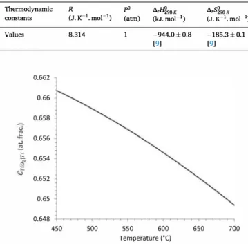
Thermodynamic constants used for Po, calculations. Thermodynamic R pO .6.r�98K constants Values 0.662 0.66 0.658
1
0.656 f_ 0.654 0.652 0.65 0.648 Table 2(J. K-1• mol-1) (atm) (kJ. mol-1)
8.314 1 -944.0±0.8
[9]
450 500 550 600 650
Temperature ('C)
Fig. 1. Evolution of Cno,in with temperature.
.6.,-�98K
(J. K-1. mol-1) -185.3±0.1 [9]
700
Values of pre-exponential factors and activation energies for O diffusion in TiO2 and Ti in the case of Ti-6Al-2Sn-4Zr-2Mo-Si alloy from Shenoy et aL [11] and Shamblen and Redden [12].
6.69-10-2 [11] 242.9 [11] 6.5·10-5 [12] 203 [12]
Second, values of the oxygen equilibrium partial pressure Po, at the oxidelmetal interface were calculated using Ellingham's approximation, following the chemical equilibrium at the oxidelmetal interface described in Eq. (12):
(12) Thus, according to Eq. (12), P02 can be expressed using the following relationship (Eq. (13)):
o (t:,,.,H°
-
T t:,,.,s-1)P0, =P •exp RT (13)
where pO is the standard pressure (in atm), àrH° the standard enthalpy
of reaction (in J.moz-1 ), àrS0 the standard entropy of reaction (in
Table 3
J.K-1.moz-1 ), T the absolute temperature (in K) and R the gas constant (in J.K-1.moz-1 ). Literature values of the previous constants [9] that were used for Po, calculations are given in Table 1. Fig. 1 shows the evolution of Cno,1n with temperature, calculated using the data in
Table 1.
Concerning O diffusion coefficients, Liu and Welsch [10] reported values of pre-exponential factors and activation energies for O diffusion in TiO2 [11] and in Ti-6Al-2Sn-4Zr-2Mo-Si [12]. These values are pre
sented in Table 2. Data relative to O diffusion in TiO2 were obtained by
fitting the oxide thicknesses measured on samples oxidized in a ther mogravimetric apparatus [11]. The parameters, pre-exponential factor DZ(n) and activation energy G0 (TI) for O diffusion within the Ti-6Al-2Sn-4Zr-2Mo-Si (Ti6242s) alloy matrix, were calculated from micro-hardness profiles performed on oxidized samples [12]. They are therefore relative to a diffusion process in a two-phase a+ � matrix.
In theory, the mass transport of the constituents on a specific sub lattice varies with the vacancy site fraction and the site fractions of the constituents. The site fractions depend on the overall composition of the phase, which in turn depends on oxygen activity (see Fig. S1 in Sup plementary Materials). The end result is that in the oxide the overall effective mass transport will depend strongly on the oxygen partial pressure, see ref. [13] for a detailed discussion on this subject. For simplification, in the present work, a constant O chemical diffusivity was used to calculate oxygen flux in the oxide scale. The microstructure of the scale may also affect the effective diffusivity in the oxide scale, as has been shown for nickel, iron or chromium oxides [14-16]. However, as long as the contribution of grain boundaries is minor and/or that there is no evolution of the scale microstructure during the oxidation, these ef fects can be taken into account by considering the kinetics parameter
Do (TiO,) as an effective diffusion coefficient in the oxide scale. 2.3. Applying the analytic models to the Ti6242s alloy case 2.3.1. Comparison with experimental data
A first evaluation of results given by these different analytic models, when applied to the high-temperature oxidation of Ti alloys, was per formed. Calculated results were compared with experimental findings as regards O diffusion profile, oxide scale thickness and mass gain. Regarding input parameters used for calculations: C110,111 was deter
mined with Eq. (11) (its value corresponds to the solubility limit of oxygen in pure Ti), activation energies and pre-exponential factors are given in Table 2. This full set of input parameter values is summarized in
Table 3.
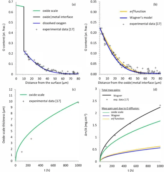
Fig. 2 presents the results obtained from the three analytic models detailed above and their comparison with experimental data. These experimental data corne from Electron Probe Micro Analysis (EPMA) measurements, cross-section analyses and mass gain measurements performed on Ti-6Al-2Sn-4Zr-2Mo-Si alloy samples oxidized up to 1 000 h at 650 °C in a 80 vol. o/o Ar / 20 vol. o/o 02 gas mixture [17]. From
Sets of initial and fitted input parameters respectively based on literature data and fitting of experimental results. General conditions Oxide Input parameters Meta! T (°C) t (h) C, (at. %) CTIO,ITI (at. %) Go(TIO,) (kJ. mol-1) vi(Tio,) (m2.s-') c,,1 Tio, (at. %) Co (at. %) vi(TI) (m2.s-1) Go(TI) (kJ. mol-1) Imposed Literature values Literature values 650 1 000 66.6 65.2 243 [11] 6.69-10-2 [11] 29.0 0 6.5·10-5 [12] 203 [12] 2nd set Imposed Literature values Fitted value Fitted values Literature value 650 1 000 66.6 65.2 243 [11] 5.4.10-2 22.4 0.355 2.4.10-5 203 [12]
C. Ciszak et al
0.7 0.35
(a) (b)
0.6 oxide scale 0.30 erf function
oxide I metal interface Wagner's model
0.5 Wagner's model 0.25 + experimental data [17] ù
�
+ experimental data [17]�
..; 0.4 ..; 0.20�
-
�
-t
C C 0.3�
0.15 :j:+ C 0 0 u u 0 0 0.2 0.10 0.1 0.05 0 0.00 0 10 20 30 40 50 60 70 80 0 10 20 30 40 50 60 70 80Distance from the surface (µm) Distance from the oxide I metal interface (µm)
12 (c) 3 (d)
11 oxide scale Wagner
+ exp. data [17]
10 + experimental data [17] + 2.5
E
9 Mass gain (;!art due to O diffusion:8 2 "'"'
"'
7 E u u 00�
"'
6 _§_ 1.5 <( ëii 5 E"'
<l "'C ·x 4 1 0 3 2 0.5 1 0 0 0 200 400 600 800 1000 0 200 400 600 800 1000 t (h) t (h)Fig. 2. 0 profiles (a) and (b), oxide scale thickness (c) and mass gains (d) obtained from analytic models using literature input data, compared with experimental data obtained in a Ti-6Al-2Sn-4Zr-2Mo-Si sample oxidized 1 000h at 650°C in a 20vol. % 0
2 / 80vol. % Ar gas mixture [17]. such specific conditions, it was possible to exclude the formation of ni
trides or N-rich a-Ti, which are known to decrease the overall oxidation kinetics [17].
According to Fig. 2, ail predictions significantly deviate from experimental data. It is therefore necessary to fit some input parameters with experimental results in order to correctly reproduce the actual behavior of a specimen. This fit was performed through a two-steps method. The first step consisted in fitting some input parameters rela tive to O diffusion in the metal (namely Cn1 no,, Co and vg(nJ) to reproduce as best as possible the O experimental EPMA profile measured in the metal. The second step consisted in fitting the effective diffusion coefficient of O in Ti02 to reproduce the experimental evolution of the oxide scale thickening as best as possible. The new input parameters obtained after this fitting procedure are presented in Table 3. Calcula tion results obtained using these data (with fitted values of Cn1 no,, Co, vg(no,J and vg(nJ) are presented in Fig. 3.
According to EPMA data, the O solubility limit should therefore also be fitted to a value close to 22.4 at. %. This lower O solubility, compared that of pure Ti, should first be due to the fact that EPMA measurements of O content are done in an a + � matrix containing 14 vol. % of�. which should dissolve tiny amounts of O. Second, the alloying elements in the a phase may change its O solubility limit. For diffusion coefficients, it was assumed that activation energies were correct, therefore only the values of pre-exponential factors were fitted. As a result, the diffusion coeffi cient of O in the metallic matrix was divided approximatively by a factor
of 2. Such variations in pre-exponential factors might be linked to the chemical composition of the a phase or to a varying contribution of short circuit diffusion paths (i.e. slightly different grain boundary and phase boundary densities) in the overall diffusion process. For either oxide scale or metallic matrix, the magnitude of short circuit diffusion is directly linked to microstructure (e.g. grain size, volume fraction of phases, phases distribution, etc.) and composition (e.g. phases compo sitions, segregation of impurity at grain boundaries, etc.). Finally, the value of Co was updated to correspond to the nominal content of O in the alloy determined by Glow Discharge Mass Spectroscopy (GDMS) [18].
With this second set of input parameters, despite a slight over estimation, the O profile given by the first mode! (simple erf function) appears to be similar to the one obtained from the two other more complete models (Wagner's mode! and Pawel's mode!).
The high-temperature oxidation of Ti alloys leads to a high propor tion of dissolved oxygen in the metal (nearly 25 at. %) that contributes significantly to the overall mass gain measured experimentally. lt is also worth noticing that, unlike the simple erf function, Wagner's and Pawel's models enable the direct comparison of calculations with experimental kinetics in terms of mass gain. From Wagner's and Pawel's models it is also possible to calculate separately each medium's (i.e. oxide and metal) contribution to the overall mass gain. Numerical cal culations as well as experimental studies confirm that none of these two mass gain contributions can be neglected (25 % in the metal versus 75 % in the oxide in the present case). These values are in agreement with
C. Ciszak et al 0.7 0.6 0.5 u
�
.;�
0.4 C ."J 0.3 0 u 0 0.2 0.1 0 0 12 11 10 Ê 9 2: 8 V> V> QI 7 u 6 5�
QI 4 ·x 0 3 2 1 0 0 (a) oxide scaleoxide I metal interface dissolved oxygen
+ experimental data [17]
10 20 30 40 50 60 70 80 Distance from the surface (µm)
(c) oxide scale + experimental data [17] 200 400 600 t (h) 800 1000 u
�
.;�
C ."J C 0 0..s
�
E <l 0.35 0.30 0.25 0.20 0.15 0.10 0.05 3 2.5 2 1.5 0.5 0 erffunction Wagner's model (b) + experimental data [17] o 10 w w � � � m w Distance from the oxide I metal interface (µm)0 Wagner + exp. data (17] 200 400 600 t (h) (d) 800 1000
Fig. 3. 0 profiles (a) and (b), oxide scale thickness (c) and mass gains (d) obtained from analytic models using input parameters adjusted to experimental data obtained in a Ti-6Al-2Sn-4Zr-2Mo-Si sample oxidized 1 000 h at 650 °C in a 20 vol. o/o 02 / 80 vol. o/o Ar gas mixture [17].
those that can be extracted from the results of Dupressoire et aL [17] (28 % in the metal versus 72 % in the oxide) after 1 000 h of oxidation under the same conditions.
2.3.2. Inffuence of the nominal O content
Since Wagner's and Pawel's models take into account the coupling between oxide scaling and diffusion within the metallic matrix, they can therefore provide the theoretical evolution of oxide scaling kinetics as a function of initial O content in the metal. For structural applications, OAZ thickness appears more critical than oxide scale thickness, because of its role in crack initiation.
Thus, being able to predict the evolution of OAZ thickness over time as accurately as possible appears to be of major interest when sizing structural components. According to Shamblen and Redden [12], a ductile to non-ductile transition occurs in the Ti-6Al-2Sn-4Zr-2Mo-Si alloy when the local O content exceeds 0.5 at. %. Consequently, the present work refers to the OAZ as the metal thickness whose oxygen content is greater than or equal to 0.5 at. %.
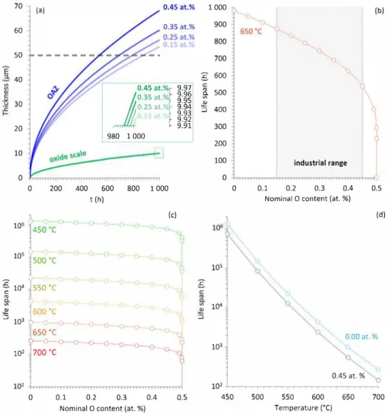
Fig. 4 presents a study of the influence of nominal O concentration on the evolution of OAZ and oxide scale thicknesses over time, using Wagner's model, for 1 000 h long oxidation tests. Calculations were performed for several temperatures ranging from 450 °C to 700 °C and for different initial O contents ranging from O to 0.5 at. % (5 000 at. ppm). The value of 0.15 at. % (1 500 at. ppm) corresponds to the nominal O content in pure Ti [19], whereas the value of 0.45 at. % ( 4
500 at. ppm) is the maximum nominal O content in commercial Ti-6Al-2Sn-4Zr-2Mo-Si alloy [20]. All input parameters used for Fig. 4
calculations are summarized in Table 4.
OAZ thickening kinetics increases significantly with the initial 0 content for the nominal O concentrations explored, i.e. from 0.15 at. % to 0.45 at. % [20] (Fig. 4a). Given the OAZ definition chosen - the part of the alloy with an oxygen concentration greater than 0.5 at. %. - this result was expected. Oxide scale growth kinetics however, is only slightly affected by the initial O content. It is worth noticing that this method also provides a means to anticipate the life span of a component based on the level of O impurity of the alloy batch. In the rest of the study, it will be assumed that beyond a relative OAZ thickness of approximately 10 % of the overall component thickness, the life span of the component falls down to zero. Based on such a criterion, an attempt was made to evaluate the life span evolution of a 1 mm thick component made of Ti-6Al-2Sn-4Zr-2Mo-Si alloy as a function of both initial 0 content and temperature.
Fig. 4b presents the life span evolution as a function of initial 0 content at 650 °C. In the range of nominal O content typically found in industrial alloys, i.e. from 0.15 at. % to 0.45 at. %, calculations show that the life span of the component would almost be halved, before drastically falling down to zero when O content cornes close to 0.5 at. %. This type of calculations could be of major interest for the development of additive manufacturing. Indeed, most additive manufacturing pro cesses recycle metal powders left over from prior build cycles. These
C. Ciszak et aL 70 (a) 60 50 40 30 20 10 0 0.45 at.% 0.35 at.% 0.45 at.% ! #.0.35 at.% Jg 0.25at.% 980 1 000 9.97 9.96 9.95 9.94 9.93 9.92 9.91 0 200 400 600 800 1 000 1 6 ( -0 ,0-lO 1450 °C s )- " 10
1
500 ·c t (h) 0-0- 0-- ,)- (c) } -Q-. �)i
10• � sso ·c1
1
�
J
6o
o
·
c
103 (}-- O (l--0- -0l
1;
c:
o
·c
o- -o o- o o- -c � 0- -0-- -0- ---0-0--0---0--- � 102 100 ·c -- - -.r---o-0 0.1 0.2 0.3 0.4Nominal O content (at. %)
0.5 1 000 900 800 700 6 600 � 500 -2! :.:; 400
6
300 200 100 0 105 104 103 0 (b) industrial range 0.1 0.2 0.3 0.4 0.5Nominal O content (at. %)
(d) 0.00 at. % 0.45 at. % 102 -1--,-,-,-,---,-,-,--,-,--,-,-,...,....,-,--,-,---,-,-,--,-,-,-.,-, 450 500 550 600 650 700 Temperature (°C)
Fig. 4. Evolution of OAZ and oidde scale thicknesses over time calculated for four nominal O contents at 650 °C for a semple with an initial thickness of 1 mm (a), evolution of the life span (see definition in the text) as a function of the nominal O content at 650 °C (b) and for different temperatures ranging from 450 °C to 700 °C (c), evolution of the life span with temperature of a material containing 0.45 at. % of O and an O free material (d).
Table 4
Set of input parameters used to evaluate life spans at 650 °C of a component as a function of its initial content in O.
Input parameters Cno,1n (at. %) C, (at. %) Cn1 no, (at. %) Co (at. %)
Values f(T) from Eq. (11) 66.6 22.4 0➔ 0.5 powders are therefore progressively enriched in oxygen over the suc cessive cycles.
As expected, temperature is the parameter that most affects life span, as shown in Fig. 4c and d. Indeed, although the O content (industrial range) can halve the component's life span, a temperature decrease of 50 °c reduces the life span of about one order of magnitude.
2.3.3. Behavior of thin components
In order to reduce the mass of certain components, hollow structures made of thin parts are often used. However, thin samples do not behave like massive samples in terms of diffusion. The mode! proposed by Pawel aims at anticipating this phenomenon. A quantitative application was proposed in a previous work [21]. The calculations were performed on a 100 µm thick sample. The same calculations are updated here using the fitted parameters (2nd set) presented in Table 3 for oxidations at 650 °c
for 73 000h.
Fig. 5 presents calculation results of O diffusion profiles in the
5.4.10-2 243 [11] 2.4.10-5 203 [12]
metallic matrix, total mass gain per unit area and its contributions ( oxide growth and O dissolution) as a function of the square root of time.
As can be seen in Fig. Sa, both mass gains per unit area (related to oxide scale formation and O dissolution), appear to follow parabolic kinetics during the first part of the experiment (until 4 00 h approxi mately). However, 0 dissolution kinetics noticeably deviates from this parabolic behavior in the second part of the experiment. This phenom enon is attributed to the progressive oxygen saturation of the metallic matrix and its subsequent consumption by the oxide growth (see
Fig. Sb). Indeed, as the metal saturates, the inward O flux progressively decreases as the metal saturates (due to the O concentration gradient decreasing), down to zero upon reaching saturation. Eventually, no more O gets into the metal while the oxide scale keeps growing. The 0 dissolved in the metal is then transferred to the oxide through the oxidation of the substrate, leading therefore to a decrease in the asso ciated mass gain.
C. Ciszak et aL (a)
���'t?c§'�
'<'-<:--<:--<:--<:--<:-",,'\, Il< <o (b) 0.25 14 12 0.2 10 : 0.15�
<t: 6 2l 0.1--
C E 4 0 0.05 2 0 0 0 50 100 150 200 250 0 10 20 30 40 50vt (hl/2) Distance from the oxide I metal interface (µm)
Fig. 5. Evolution of calculated mass gains with the square root of time for a sample of 100 µm initial thickness according to calculations with Pawel's mode! for 73 000 h of oxidation at 650 °C (a) and evolution of the O diffusion profile within the metallic matrix (progressively consumed by the oxide growth) for the same sample (b).
are correlated phenomena, it is worth noticing that Wagner's and Pawel's models do not predict any feedback effect on the oxide scaling kinetics. Wagner's and Pawel's models predict no evolution of the mass gain kinetics related to the oxide growth when decreasing the sample thickness, although a strong difference appears for the metal part evo lution (Fig. Sa). The explanation of such a behavior lies in Eq. (7), from which the value of y is extracted. Indeed, the primary mathematical problem was established for initial and boundary conditions assumed constant, including parameter C0• However, for a sample with finite dimensions, Co will eventually increase over time, when the O diffusion profile reaches the middle of the sample and until total saturation of the metal (defined by Cn1 no2). Consequently, this should inevitably impact
the associated value of y, which describes scale growth kinetics. Pawel's model does not take into account the influence of this evolution to es timate the y parameter. As a result, although this model was designed to take into account the effect of a finite size sample on the O diffusion in the metal, it does not consider the influence of oxygen saturation in the metal on oxide scaling kinetics. Hence none of these analytic models provide an accurate analysis of the oxidation of thin samples.
First, analytic models suffer from limitations for application cases in which oxidation conditions (time and temperature) lead to an O diffu sion profile that will not reach the middle of the sample. Second, the analytical models cannot take into account temperature transients, local evolution of diffusion coefficients, local evolution of the volume frac tions of phases and redistribution in the alloying elements, which can be key factors in certain applications. With the objective of mitigating these limitations, numerical approaches were developed.
Table 5
Initial and boundary conditions set for the oxide and metal media. Medium Oxide Meta! Index i = l 1/i E ll;n] i =n+l j=m 1/j E lm;m+q-1] j =m+q Abscissa z =zi . z'+l_z' z =z'+- -2-z = z' z = zj . zj+l_zj z =zl+--2 -z = zj
3. Numerical modelling of the high-temperature oxidation of Ti alloys
Most numerical models involving O dissolution have been developed for high-temperature oxidation of Zr-alloy claddings used in the nuclear industry. Similar approaches can be adapted to Ti alloys. In the next section, after a short review of the existing models, a numerical tool called PyTiOx, which was designed to model the oxidation of titanium alloys, is detailed.
3.1. Available numerical tools
A few numerical tools have been developed over the years to model the high-temperature oxidation of metals. Among them, FROM [22],
SVECHA [23], DIFFOX [24], and EKINOX-Zr [13,25] can be cited as numerical models dedicated to the high-temperature oxidation of Zr-alloys. They all use finite differences algorithms based on the solving of Fick's laws in a 1D system that is considered either in Cartesian co ordinates [22,25] or in cylindrical coordinates [23,24]. All of them support interface displacements. However, they differ in several aspects. On one hand, only the SVECHA and FROM models allow for O interfacial concentrations to be out of the thermodynamic equilibrium. On the other hand, the DIFFOX and the EKINOX tools support multi-phased materials, such as a stratified oxide scale or a two-phase metallic matrix. Another numerical method, based on a finite volume method, was proposed by Kitashima et al. [26] to mode! the high-temperature oxidation of a-Ti under isothermal conditions. This mode! also sup ports the displacement of the oxidelmetal interface, but the rate of the
Initial conditions Boundary conditions
xo (z,t= to) = C, x0 (z, t > 0) = C,
x'o (z,t=to) =C,-e,f( 2JDo (no,)t z ) (C,-Cno,1n)erfy xo (z, t = to) = Cno,1n I xo (z, t > 0) = Cno,1n Xo (z, t > 0) = Cn1no, Xo (z, t = to) = Cn1no, xi0 (z,t= t0) = erfc( �)
(C"?�))
+Co
2yDo(n1t erfc Y____'P_
Jo (z, t = t0) = 0 p
I Jo (z, t > 0) = 0
C. Ciszak et al
lJ
(ox)1�
(ox)c.
0 X,5 (ox) oxide·
·
·
//
···//
n-1 Xo {ox) z'fix 018cJx)
J:J\met) CriO,ITi Cr;irw2 metall'ff
t;iet)�--�·-···//··
m+q-1 la (met) x0 linearly interpolated EB Xo + la x···//
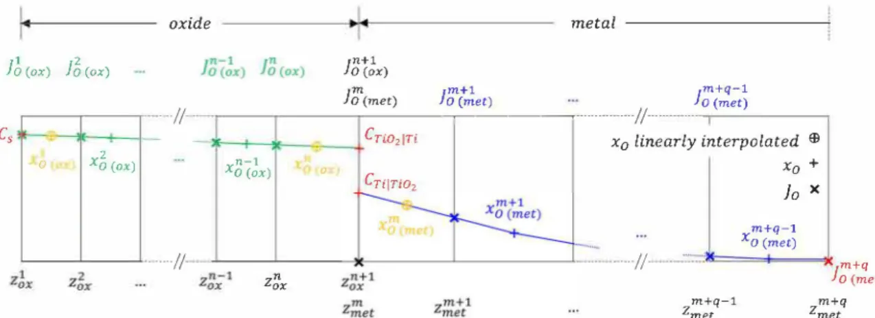
m+q-1 Xo (met) m+q la (met) m+q-1 2met 2met m+qFig. 6. Schematic representation of the system configuration in the PyTiOx mode!. interface recession is calculated from an experimental law accounting
for the oxide scale growth kinetics. Therefore, Kitashima's model allows for the oxygen diffusion profiles within the metal to be calculated with the evolution of the oxygen content at the metalloxide interface over time and with temperature, but it does not take into account the feed back effect previously mentioned, i.e. the influence on scaling kinetics of oxygen dissolution in the metal. The present work aims at developing the same kind of approach proposed for Zr-alloys, but applied to the specific case of high-temperature oxidation of Ti alloys.
3.2. Development of a new nwnerical tao/: PyTiOx
A new numerical tool called PyTiOx was developed based on the numerical scheme of explicit finite differences applied to a 1D calcula tion domain. The system is composed of two media: one corresponding to the metal and the other to the oxide scale with an initial thickness of ,;0, which is taken as small as possible to simulate the oxidation of an initially unoxidized alloy. The two media are treated separately. Each medium is divided into slices: the oxide into n slices and the metal into q slices. The meshes of the oxide and of the metal are anchored in their respective crystallographic lattice. Therefore, the slices inside the oxide and inside the metal do not move relative to the oxide and metal lattices respectively, but the oxide and metal meshes move relative to each other. A moving interface algorithm enables to describe the growth/ thinning of the oxide scale and the corresponding metal recession/ growth.
The O concentration in each slice "i" is designated as xi0 (medium)"
Table 5 presents the initial and boundary conditions set for the oxide and
the metal media. The boundary conditions used for the following application of the numerical model are the same as those chosen in Wagner's analytical model for the concentration at oxide surface (C,) and at the metalloxide interface (Cr;o,1n and Cn1no2). As in Wagner's mode!, these two interfaces are considered to be at the local equilibrium. To integrate fini te size samples, the boundary condition at the last metal slice on the right side, i.e. the center of the sample, is a null flux
(J0 (z = zm+q, t
>
0) = 0). According to Eqs. (6) and (7), the actual initial time to is recalculated based on the oxide thickness ,;0 initially set, so that the thickness of the oxide and of the OAZ have a value of O at time t=
O. This value of to is then used to calculate the corresponding initial oxygen diffusion profile in each medium, using Eqs. (2) and (3) for the oxide and the metal, respectively.Fig. 6 presents a schematic representation of the system configura
tion. Values of boundary conditions presented in Table 5 can only change with temperature. They were therefore considered constant in the calculations under isothermal conditions.
At each time step t.t, 0 transport between slices is calculated using 0 fluxes, J0, from the following equations (Eqs. (14)-(16)):
For i
=
IVi E ]l;n]
(; ) JO (ox) ,
=
-Do (ox) !(i+l _ (.io(ox)), -C, 2 (ox) (ox) ti )
( ; )
(X�
(ox) -x�/ox))la (ox) ,
=
-Do (ox)" 1 ( ;+1 _ ;_1)2 z(ox) z(ox) t ·
(JO (met) -J;/me,))
Vj E [m+l;m+q-1] (J'o(met)),=-Do(met)" !(z+l -t,-1) 2 (met) (met)
(14)
(15)
t
(16)
The flux balance, performed for each slice using the fluxes previously determined at time t, allows for the explicit treatment of the O mass
balance in each slice at time t + t.t, according to the following re lationships (Eqs. (17) and (18)):
· i+l
ViE[2·,n-l]:(; )
=(;
+I'o(ox)-JO(ox))•t.tXo (ox) t+<l>t Xo (ox) Z;+1 ; (ox) -Z(ox) t
j j+l
(17)
v1· [ E m+ l;m+q-l : O(
l
(:i. met) t+àt )=
(1
O(met)+
JO (t,+1 met) -JO (-t,
met)) •f.t (met) (met) t(18)
The algorithm for the displacement of the metalloxide interface re lies on the growth and thinning of the slice of each medium that is adjacent to the metalloxide interface. The algorithm of growth and thinning is based on a mass balance considering fixed concentrations at the metalloxide interface Cn1no, and Cno,1n• Assuming a linear inter polation of the O concentration profile in the first slice of each medium adjacent to the metal I oxide interface, the total O quantity Qo (w<) present in the slices "n" and half of "n -l ", "m" and half of "m + 1" can be expressed as follows:
(Qo (tot)), = (Qo (ox)
+
Qo (met)), With: (Qo(me1)), =G (
Cn1rw,+�ê!,,)) (
t.Z:e,+
è,.zF)),
Vi E [1; n] : f,.z�x=
z�t1 -Z�x Vj E [m;m+
q- 1] : t.z!me, = i,,;,) -ime, (19) (20) (21) (22) (23)C. Ciszak et al (a)
���'t?c§'�
'<'-<:--<:--<:--<:--<:-",,'\, Il< <o (b) 0.25 14 12 0.2 10�
E : 0.15�
oi, -..§. <t: 6 C 0.1--
E 0 4 0.05 2 0 0 0 50 100 150 200 250 0 10 20 30 40 50{f (hl/2) Distance from the oxide I metal interface (µm)
Fig. 7. Comparison of the evolution of numerically and analytically (Fig. 5) calculated mass gains as a function of the square root of time for a 100 µm thick sample using Pawel's and PyTiüx models for 73 000 h of oxidation at 650 °C (a) and evolution of the O diffusion profiles within the metallic matrix (progressively consumed by the oxide growth) relative to a 100 µm thick sample (b ).
Then, considering the mass balance from O fluxes getting in the last oxide slice and a half adjacent to the metalloxide interface, and out of the first metal slice and a half adjacent to the metalloxide interface:
(t.Q ) 0 t
= (
1naO (ox) ,1n _ 10 (met) t n1Tw,) .t.f (24)With
J�f;;f
i and J�1(:�:), the oxygen fluxes in the middle of the slices n -1 andm+
1, respectively:r +r-'
1no21r; _ 0 (ox) 0 (ox)
O(ox) - 2
J':!.+1 +J':!.+2
1nino2 _ 0 (met) 0 (met)
O(met) - 2
(25) (26)
At each time step, the displacement of the metalloxide interface re sults from the change in size of the slices that are on each side of the interface.
The size of the metal and oxide slices that are next to the interface are calculated from the oxygen mass balance using Eqs. (19)-(26), and using the mass conservation of Ti, which imposes the following relationship
(a) 30 25 20
E
u oi, 15 ..§. <t:--
<I E 10 5 0 - 200 µm thick...
100 µm thick�
.._,ol\:...
.
••.
.
,.;r-
·
�o
e .-,;• 0,
,
f.
·
,,.
..
meta/ 0 50 100 150 200 250 300 350 400 {f (hl/2) (Eq. (27)): t.i,;, (t+àt) - t.t,;, (t)=
P ( t.Z:et (t) - t.Z:::,t (t+àt)) (27)Eq. (27) links the change in size of the oxide and metal slices that are on each side of the interface to the PBR of Ti/Ti 02, i.e. the ratio of the molar volume of Ti in the metal to the molar volume of Ti in the oxide. In order to minimize calculation errors due to large slices, the displacement of the metalloxide interface is also modelled by an algo rithm that creates or deletes slices in each medium, on both sides of the interface. A growing slice exceeding !t.z<l is split into two new slices: a first one of t.zÜ thickness and a second one of the remaining thickness.
Analogously, a thinning slice becoming thinner than
½t..z
0 is merged with the adjacent slice of the same medium (where t.z0 is the initial thickness of the slices).This algorithm allowing to solve the moving boundary problem is the same as the one used in several previous works for various simulations with multicomponent diffusion-controlled reaction under local equilib rium. These works concern the kinetic demixing of an oxide solid solu tion [27], phase transformation under transmutations studies [28], Zr alloys oxidation studies [3,13,25,29] and chromino-former Ni-base (b)
E
u oi, ..§. <t: --<I 30 25 20 15 10 kp = 5.5·10·3 mg2.cm·4s1 ,,/�
,,/
,,,,,,,
,'/
/,,,,
,/' 5 ,/ /// kp = 2.9·10·3 mg2.cm·•s1 0 50 100 150 200 250 300 350 400 {f (hl/2)Fig. 8. Overlay of the calculated mass gains per unit area using the PyTiüx mode! for the oxidation oftwo different sample sizes (100 µm and 200 µm thick) at 650 °C (a) and focus on the two successive parabolic regimes forming the oxide growth kinetics curve (b).
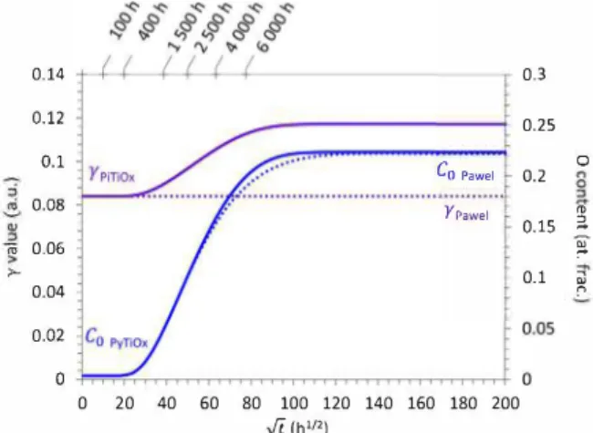
C. Ciszak et aL 0.14 0.12 0.1 0,08 rn 0.06 ;,.. 0.04 0.02 0 0 Co Pawel Y Pawel 20 40 60 80 100 120 140 160 180 200 ,/f (h''') 0.3 0.25 0,2 0.15 0.1 0 (1) a'.
�
�
Fig. 9. Evolution of rand Co over time calculated from Pawel's and PyTiOx models for a 100 µm thick sample.
alloys alloy oxidation studies [15,30-32]. This algorithm is perfectly adapted to the explicit finite differences time integration algorithm. A convergence study was performed prior to first calculations allowing to correctly choose the time and space calculation steps (0.857 s for the time calculation step and 0.5 µm and 0.1 µm for space calculation steps in metal and oxide respectively). The algorithm was tested and it correctly reproduces analytical solutions when they exist (See Fig. S2 in the Supplementary Materials). Other works, such as [33], propose different algorithms with an interfacial region that extends to the same depth for both phases. These algorithms also seem to be efficient for various simulations of diffusion-controlled reactions under local equi librium conditions. In this latter work however, the variation of the molar volume between the two phases is not explicitly taken into ac count in the moving equation. This cannot be neglected in the case of oxidation which involves important volume changes and where both diffusion in the metal and in the oxide had to be treated. A third solution could be to use the new Sharp Phase Field Method, described by Finel
et aL [34]. This would also be more efficient in terms of calculation time.
However, the explicit finite difference algorithm together with the moving boundary algorithm described here were well suited to the simulations presented in this study.
3.3. PyTiOx results
This section presents the results obtained from PyTiOx calculations for different real-cases applications. The aim is to study quantitatively the influence of sample size (thin wall component) and thermal transient on the behavior of titanium alloys in high-temperature oxidizing conditions.
3.3.1. Swnple size effect
Fig. 7 illustrates the calculations performed using the PyTiOx model on a thin, 100 µm thick sample, oxidized 73 000 h at 650 °c. The input data are the same as those used for the calculations performed previ ously for the same conditions (summarized in Table 3 set 2) using Pawel's analytical model (Fig. 5). The results from Pawel's and PyTiOx models are overlaid to be compared.
PyTiOx calculations show that the growth kinetics of the OAZ and of the oxide scale are both affected by the progressive oxygen saturation of
Table 6
the metal, which occurs at longer durations. The oxide scale growth kinetics appears to be higher than its initial parabolic growth rate. Ac cording to Fig. 8a, the thinner the sample is, the earlier this deviation happens. It appears at about 400 h and 20 000 h for 100 µm and 200 µm thick samples, respectively. In agreement with Fig. 7b, this occurs when the metal becomes saturated in 0, evidencing a kinetic transition. Indeed, contrary to analytical models, this numerical model accounts for the feedback of the O content evolution at the center of the sample (Co) on the oxide scaling kinetics. The scaling kinetics of thin samples thus follows two successive regimes. The first one is effective for short oxidation times and is limited by the diffusion of O in both the oxide and the metal. According to Fig. 7a and b, the second one becomes effective once the metal reaches oxygen saturation. At this stage, the O fluxes in the metal decrease to zero, because the O concentration gradient in the metal tends towards zero. Therefore, the entire O flux within the oxide scale is consumed to grow the oxide scale. This is corroborated by
Fig. 7a. The oxide scale growth kinetics switch from a first parabolic regime to a second, faster one (Fig. 8b). During the first parabolic regime, the scaling kinetics is controlled by the oxygen flux trough the oxide scale minus the oxygen flux transferred to the metal. During the second one, the scaling kinetics is controlled by the entire oxygen flux crossing the oxide scale and reaching the oxidelmetal interface.
Fig. 9 presents the evolution of the O content (Co) over time at the center of a 100 µm thick sample, provided by both analytical (Pawel's model) and numerical (PyTiOx model) resolutions. The corresponding values of the r parameter, which describes scale growth kinetics, is also shown. In the PyTiOx model, y values are calculated using Eq. (7) at each time step. Three stages can be distinguished. The first stage, defined by the first dwell of each curve, corresponds to the parabolic oxidation kinetics of a semi-infinite material containing a nominal O content, C0•
The beginning of the second stage occurs when Co starts increasing. It corresponds to a kinetic transition which is directly linked to the evo lution of the y parameter. In the present case, an increase in the scaling kinetics is observed concomitantly with the increase in Co and y, ac cording to PyTiOx results. A third stage then appears once Co reaches its maximum value, which corresponds to Cn1 no,: the O solubility limit of
the material. Hence the scaling kinetics (i.e. the oxide growth) follows a parabolic growth during a first stage, then a transitory stage toward a second accelerated parabolic growth rate (second dwell with constant value for y). The deviation of the results calculated using Pawel's model from those calculated using the numerical model is evidenced in Fig. 7
and shows the limits of application of this analytical model. 3.3.2. Thermal transient
All the previous numerical and analytical calculations were done in isothermal conditions. However, real in-service conditions involve at least two temperature transients, corresponding to the heating and cooling steps of materials. Most industrial high-temperature equipment is thermally cycled. Analytical models are not suitable for such non isothermal cases. The numerical model PyTiOx is however able to integrate non-isothermal conditions.
A complex temperature transient, schematically close to the real operating conditions undergone by a component in an aircraft engine made of Ti-alloy, was selected to evaluate the relative contribution of each temperature segment on the overall oxidation process. The input parameters for this calculation are summarized in Table 6.
To avoid excessively long computing times, the lowest temperature was set to 250 °C, assuming that contributions at lower temperatures can
Set of input parameters used for calculations in non-isothermal conditions ("~" means that the values of the corresponding parameter vary).
Input T t (h) h (m) C, (at. C,10,111 (at. C111 no, (at. Co (at. vg(,,o,J (m2. Go
(TIO,) vg("l (m2. Go(TI)
parameters ("C) %) %) %) %) s-') (kJ. mol-1) s-') (kJ. mol-1)
C. Ciszak et al 600 'C 0.025 600 525
·c
550 0.02 500 450 400 E 0.015 350 <.> ... bb oxide 300rl
.s
<( 250 ---- 0.01 200 150 0.005 100 50 0 0 0 1 2 3 4 5 6 7 8 9 t (h)Fig. 10. Evolution of mass gains per unit area over tirne in non-isotherrnal conditions. 90 600 0.9 80 T 550 500 0.8 70 oxide 450 0.7 � 60 400 -" 0.6 "' OAZ 350 ::l
.§
50 ... "' 300 � 0.5�
.d
�
40 250 -E 0.4�
N 30 200 <( "' 0 0.3 150 0.2 20 100 0.1 10 50 0 0 0 0 2 3 4 5 6 8 9 1 (h)Fig. 11. Evolution of oxide scale and OAZ thicknesses over tirne in non isotherrnal conditions.
be neglected. Fig. 10 presents the evolution of the different mass gains per unit area over time and temperature. In the present case, the ma terial's oxidation behavior appears to be significantly influenced only during the three high-temperature dwells at 600 °C, 535 °C and 525 °C. Despite a few additional variations during the overall thermal transient, the magnitude and/or duration of these thermal variations seem to be too low to significantly influence the oxidation behavior of the sample.
Fig. 11 presents the evolution of oxide scale and OAZ thicknesses over time and temperature. First, the thickening of the oxide scale and the OAZ is noticeably effective only during the first short dwell at 600 °C; the two following dwells at 535 °C and 525 °C appear to have only a small effect on the oxide scale growth. Second, when the tem perature drops down significantly and quickly before stabilizing for a relatively long duration, the oxide scale is then slightly reduced before starting to regrow. This temporary reduction of the oxide is due to a change in the flux balance at the metalloxide interface (Eq. (24)) when the temperature drops. A similar phenomenon was previously predicted and observed [25,29] on Zr alloys under particular conditions by Mazères et al. In Mazères's work, the conditions explored reproduced a hypothetical scenario of loss-of-coolant-accident affecting claddings of a pressurized water reactor, involving a fast temperature increase from 320 °c to 1 200 °c. In the case of Zr alloys, the partial reduction of the oxide scale was attributed to the fact that as temperature rises, the ox ygen solubility in the metallic matrix increases as well.
In the present case of the Ti alloy, the phenomenon is not due to a change in solubility limit with temperature, but to a change in diffusion coefficients with temperature in both the oxide and the metal. Indeed,
3.10-10 E 3·10·11 C: 0 ·-e T 3·1O·l3 +-rm-rr..-m..-m-rr;-r,-rr.,-m-rrm-rr..-rr+ 0 0.25 0.5 o. 75 1 1.25 1.5 1. 75 2 t (h) 600 550 500 450 400 350 300 ... 250
.d
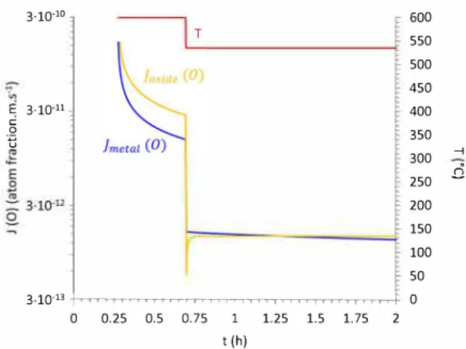
200 150 100 50 0Fig. 12. Evolution of oxygen fluxes getting out of the oidde (orange) and get ting into the rnetal (blue) as a function of tirne during the ternperature transient frorn 600 °C to 535 °C. (For interpretation of the references to colour in this figure legend, the reader is referred to the web version of this article.) the partial reduction of the oxide can be easily explained through the
. fl TiO,ITi d JTilTiO, h 'd f th
evolut10n of local oxygen uxes J0 (ox) an O (met) on eac s1 e o e
oxidelmetal interface. Fig. 12 presents the evolution of these oxygen fluxes as a function of time during the temperature transient from 600 °C down to 535 °c. The activation energy of oxygen diffusion in the oxide (G0 (no,)= 243 kJ.mol-1) is higher than in the metal (Go (Ti)= 203 kJ.
mol-1). This implies that the diffusion coefficient of oxygen in the oxide is more sensitive to temperature changes and therefore so is the asso ciated oxygen flux in the oxide. In the present case, the quick temper ature drop from 600 °c down to 535 °C causes the oxygen flux getting out of the oxide to be temporarily lower than the one getting into the metal. The oxygen flux in the oxide reaching the oxidelmetal interface is then no longer sufficient to sustain oxygen diffusion in the metal. Considering the equilibrium conditions at the interface, this leads to a partial reduction of the oxide scale until the flux balance at the oxidel metal interface becomes positive again. Such a condition is progres sively reached, because the O flux in the metal decreases with its con centration gradient, coupled with the O flux in the oxide that remains high, because of the very low growth of the oxide scale during the lower temperature dwells. The oxide scale then starts re-growing parabolically until any new thermal perturbation occurs.
As far as titanium oxidation is concerned, such a phenomenon has never been evidenced experimentally nor reported. However, the pre sent calculations show that, under the conditions explored here, this phenomenon is rather insignificant. It is difficult to anticipate what it might imply in terms of mechanical degradation. This phenomenon could lead to the temporary formation of a saturated a-Ti(O) area be tween the oxide scale and the remaining metallic matrix. Formation of such a brittle phase, perhaps porous because it results from the reduction of an oxide phase, might noticeably affect the mechanical properties of the component, favoring crack initiation conditions already induced by the oxidation of the material.
Fig. 13 presents the evolution of mass gains per unit area over four consecutive thermal cycles. It indicates that the material behaviour is slightly different during the thermal cycles that follow the initial one, confirming the transient nature of the first cycle.
Fig. 14 presents the evolution of OAZ and oxide scale thicknesses as a function of the square root of the number of thermal cycles for 16 thermal cycles. According to Fig. 14, OAZ and oxide scale thicknesses evolution over time follow parabolic laws over the number of thermal cycles as long as the sample does not start to saturate in oxygen. The growth rate is much higher for the OAZ than for the oxide scale. The parabolic rate constants are respectively 0.97 µm.nb;;,1/i: for the OAZ, and 9.0-10-2 µm.nb;;.1/i: for the oxide scale. For pratical purposes, it is
C. Ciszak et al 0.05 T 0.04
5
0.03 <( Ê 0.02 total oxide 0.01 0 0 5 10 15 20 25 30 t (h) 35 600 550 500 450 400 350 -, 3006
250 200 150 100 50 0Fig. 13. Evolution of mass gains per unit area over time for 4 thermal cycles.
4 �'\,, 0,0 0 0 3.5 0 0 .0 0 3 0 0 Ê 2.5 0 0
�
0 2 0 C5 1.5 f- 0 1 cf 0.5 oxide 0 0 0 0 0000000000 0 0 0 0 1 2 3 4 (Number of cycles) 112Fig. 14. Evolution of OAZ. (blue) and oxide scale (green) thicknesses with the
square root of the number of thermal cycles. (For interpretation of the refer ences to colour in this figure legend, the reader is referred to the web version of this article.)
interesting to calculate the equivalent isothermal oxidation treatment that would give the same parabolic rate constants. This was applied to the present case; results show that an isothermal oxidation at a tem perature of 538 °C would lead to the same OAZ growth rate and an isothermal oxidation at a temperature of 546 °C would lead to the same oxide scale growth rate. Again, these values show the important contribution of the short period at 600 °C over the entire cycle. Of course, ail these considerations are only valid if the metallic matrix does not undergo any significant metallurgical evolution.
4. Conclusion
The aim of this work was to study the influence of different features on the high-temperature oxidation behavior of titanium alloys based on O diffusion modelling. A new 1D finite differences numerical mode! which includes boundary displacement, has been developed for Ti-alloys oxidation. The model's input parameters are the O diffusion coefficients in the alloy and in the Ti oxide phase, along with the equilibrium con centration at the oxidelgas and meta!loxide interfaces. Output data are: the oxygen concentration profiles in the two phases as well as the oxide growth and the metal recession.
For a given sample, it is therefore possible to calculate which pro portion of its mass gain is attributable to oxide scale growth and which
proportion is attributable to O diffusion in the matrix.
In the calculations carried out in this study, the input parameters were chosen in order to reproduce the literature-based experimental data obtained on Ti-6Al-2Sn-4Zr-2Mo-Si alloy. For this alloy, the Oxygen Affected Zone (OAZ) thickness, deduced from the O concentration pro file calculations, was defined as the part of the alloy with over 0.5 at. % of O. This corresponds to the brittle region found in previous literature results. With this definition, it was possible to follow OAZ growth ki netics as a function of different parameters and oxidation conditions.
First, it is important to state that ail calculations show that, even though O diffusion in the alloy only accounts for 30 % to 50 % of the total mass gain, the OAZ depth in the alloy is significantly thicker than the oxide scale. This is of major concern as far as embrittlement is concerned.
Second, the effect of nominal O concentration on the theoretical life span - when the latter is controlled by OAZ thickness - was deduced from analytical calculations for a typical wall thickness of 1 mm. It shows that depending on the nominal O concentration of the alloy batch, ranging from 0.15 at. % to 0.45 at. % (1 500 at. ppm to 4 500 at. ppm), the theoretical life span estimated from the OAZ depth in relation to the sample thickness, can be divided by two. The results also give an esti mation of the life span's order of magnitude at in-service temperatures: typically, only one thousand hours at 650 °C to ten thousand hours at 500°C.
Third, it was shown that the new numerical tool - PyTiOx - can overcome certain limitations relative to analytical models. The case of thin samples or thin parts is important, especially for additively manu factured components. Results from numerical models show that Pawel's mode!, which consists in a few modifications of Wagner's mode! that captures the treatment of finite size samples by analytical approxima tion suffers from a Jack of consistency. It does not reproduce correctly the �oupling between oxide growth and O diffusion in the alloy once the O diffusion profile reaches the middle of the sample. In this case, the numerical mode! should be used. Through this method, it is possible to calculate the increase in oxide scale growth kinetics as the substrate becomes richer in oxygen.
Fourth, the numerical mode! was used to calculate the oxidation induced by a temperature transient similar to the conditions undergone by an aircraft engine component. Results show that the shortest time dwell, corresponding to the take-off stage, which is when the tempera ture is the highest, has the strongest effect on OAZ and oxide scale growth. However, calculations also revealed that the longer dwells corresponding to cruise stages cannot be completely neglected. Calcu lations over several cycles also confirmed that the OAZ thickness follows a parabolic evolution with the number of thermal cycles, the parabolic rate growth of the OAZ being about 10 times higher than that of the oxide scale in these conditions.