Differential Explanations for Energy Management in Buildings

HAL Id: hal-01576282

https://hal.archives-ouvertes.fr/hal-01576282

Submitted on 23 Aug 2017

HAL is a multi-disciplinary open access

archive for the deposit and dissemination of

sci-entific research documents, whether they are

pub-lished or not. The documents may come from

teaching and research institutions in France or

abroad, or from public or private research centers.

L’archive ouverte pluridisciplinaire HAL, est

destinée au dépôt et à la diffusion de documents

scientifiques de niveau recherche, publiés ou non,

émanant des établissements d’enseignement et de

recherche français ou étrangers, des laboratoires

publics ou privés.

Differential Explanations for Energy Management in

Buildings

Amr Alzouhri Alyafi, Monalisa Pal, Stephane Ploix, Patrick Reignier,

Sanghamitra Bandyopadhyay

To cite this version:

Amr Alzouhri Alyafi, Monalisa Pal, Stephane Ploix, Patrick Reignier, Sanghamitra Bandyopadhyay.

Differential Explanations for Energy Management in Buildings. Computing Conference 2017, SAI, Jul

2017, Londres, United Kingdom. �hal-01576282�

Differential Explanations for Energy Management

in Buildings

Amr ALZOUHRI ALYAFI

Monalisa PAL

Stephane PLOIX

Patrick REIGNIER

Sanghamitra BANDYOPADHYAY

August 22, 2017

Abstract

In the field of building energy efficiency, researchers generally focus on building performance and how to enhance it. The objective of this work is to empower the building occupants by putting them in the loop of effi-cient energy use, supporting them to achieve their objectives by pointing out how far their actions are from an optimal set of actions. Different levels of explanation are investigated. Indicators measuring the distance to optimality are, firstly, proposed. An algorithm that generates deeper explanations is then presented to determine how changing some actions impacts comfort. The paper emphasizes the importance of explanations with a real case study. It identifies the type and level of explanations needed for different occupants. The concept of replay is presented. An occupant can replay his past actions and learn from them.

Keywords: building; efficient energy use; exploration of differential expla-nations; causality; multi-objective optimization; differential evolution; Pareto-optimality; ambient intelligence; user advice generation

1

Introduction

Considering the massive increase in energy demands, building consumption is a very fundamental domain as it constitutes more than 40% of the globally

sup-∗_{GSCOP, Grenoble Institute of Technology, 46 avenue Felix Viallet, Email:}

amr.alzouhri-alyafi@imag.fr

†_{Indian Statistical Institute 203, Barrackpore Trunk Road, Kolkata - 700108, India Email:}

monalisap90@gmail.com

‡_{GSCOP, Grenoble Institute of Technology, 46 avenue Felix Viallet,}

Email:stephane.ploix@grenoble-inp.fr

§_{Univ. Grenoble Alpes, CNRS, Inria, Grenoble INP, LIG, 38000 Grenoble, France,}

Email:patrick.reignier@inria.fr

¶_{Machine Intelligence Unit Indian Statistical Institute 203, Barrackpore Trunk Road,}

plied energy [1]. It illustrates the importance to decrease or limit the emissions from buildings. Enhancements in construction techniques, insulation and build-ing regulations have increased the relative energy impact of occupant’s actions in the energy consumption. It is therefore important that occupants under-stand the impact of their actions in order to reduce the energy consumption while meeting their demands on expected comfort.

An energy management system with explanatory capabilities relies on phys-ical models. These models are used to simulate and predict the evolution of various variables (temperature, air quality, consumption, etc.) according to ac-tions. Depending on the service provided by the occupants, the models can be used in a direct way for simulating an action’s impact, or in an indirect way to compute the best actions according to some criteria. Due to their complexity and mathematical formalism, models and optimization results are however not suitable for direct interactions with inhabitants: the intrinsic knowledge they contain is not directly intelligible. Human beings are trained, since elementary school, to think and to understand the world through causal representations like: what happens, when does it happen, what affects it, and what does it affect? [2]. This causal knowledge is hidden inside the equations and should be explicit.

The paper focuses on the generation of explanations about energy impact of user actions. Explanations occur in different ways [3] and for different reasons. One of the main motivation for having explanations is to be able to manage in a better way if similar events or scenarios arise in future [4]. Explanations usually rely on causal relationships. There are at least four kinds of causal explanations: common cause, common effect, linear causal chains, and causal homeostasis (cyclic causal relationships) [5]. According to [6], explanations are ubiquitous, come in a variety of forms and formats, and are used for a variety of purposes. Still, the common feature about most explanations is their limitation. For most natural phenomena and many artificial ones, the full set of relations to be explained is complex and far beyond the grasp of any one individual.

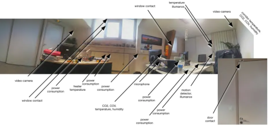
The paper focuses on a real case of study: an office, where 4 persons work. It is equipped with 27 sensors collecting information about CO2 concentration,

humidity, electrical consumption, luminescence, temperature, presence, occu-pancy etc. It is also equipped with 2 cameras to verify the occupant’s actions and their routines in historical data. A panoramic photo of the office with sensors is presented in Fig. 1.

The comfort criteria for this office are the thermal comfort and the air quality based on CO2. The office does not contain any controllable HVAC system. This

work proposes a method for occupants to better understand and learn how to improve their actions. In this scenario or similar ones, changing the door and window positions are the only possible actions occupants may perform. Such an application in energy building is first of its kind, as par the author’s knowledge, and here lies the novelty of the proposed work.

The next section shows a brief description of the problem and a general approach to resolve it. Section 3 describes the motivation for generating expla-nations for energy management systems while presenting the physical models.

video-camera video-camera CO2, COV, temperature, humidity microphone power consumption power consumption power consumption power consumption power consumption power consumption door contact window contact window contact motion detector, illumance illumance temperature heater temperature corridor temperature, CO2, COV, humidity

Figure 1: Panoramic photo of the office with sensors

Section 4 proposes a new indicator that helps the occupants to understand the gap between their actions and optimal actions according to comfort criteria. Section 5 focuses on how to show to the occupants the consequences of their actions as compared to optimal actions, by generating differential explanations and influences.

2

Problem Statement

The main objective of the paper is to propose solutions to assist occupants to better understand how they can modify their behavior and make better decisions with respect to their own comfort criteria. Due to the complexity of the building physics and unconscious routines, occupants face difficulties while trying to understand what is happening and why they need to change their daily routines to obtain better comfort, or to better compromise between comfort and cost. Generation of contextual explanation is therefore at stake.

Explanations should rely on causal relationships i.e on an ordering in phe-nomena modeled by variables: the causes, i.e. the occupant actions (A) or contextual (C) phenomena, the final effects (E) and the intermediate effects (I). It is summarized in Fig. 2 for the studied office. The arrows in the figure represent the cause-effect relation between these groups.

The different groups of variables are given by:

1. Context group: it contains all the uncontrollable variables that the system needs to take into consideration like the outside temperature Tout, the

humidity, the temperatures in the neighbor zones Tcor, the number of

occupants, etc.

2. Actions group: it contains all the different actions that the system can propose to the occupants to enhance their comfort levels (like opening the window ζw, and opening the door ζD).

Figure 2: General schema of explanations

3. Effect group: it contains the variables that will be directly experienced by the occupants like thermal dissatisfaction σT and air quality dissatisfaction

σair.

4. Intermediate group: it contains different sub-groups and different levels for multiple intermediary variables. These variables are either measured like the indoor temperature Tinand the indoor CO2concentration Cinor

estimated like the heat flow ϕheat and the air flow ϕair.

All of this can be reformulated as: A, C−→ E where:I A is the set of variables modeling occupant’s actions, C is the set of contextual variables,

I represents the intermediate variables, and E represents the effect variables.

The effects resulting from the best actions according to some given criteria can be computed.

It is denoted by: A∗, C I

∗

−→ E∗ where: A∗ is the optimal set of actions,

I∗ represents the intermediate variables generated from optimal actions, and E∗is the optimal effects that can be achieved.

To generate the explanations, a concept of a qualitative distance is defined by comparing the actual scenario (˜x) to the optimal one (x?_{), which is given by:}

Πv−3,v−2,v−1,v1,v2,v3(x ? − ˜x) : x?− ˜x < v−3 → very low v−3≤ x?− ˜x < v−2→ low v−2≤ x?− ˜x < v−1→ slightly low v−1≤ x?− ˜x < v1→ no change v1≤ x?− ˜x < v2→ slightly high v2≤ x?− ˜x < v3→ high x?− ˜x ≥ v3→ very high (1)

This mapping is done to show the occupants the impact of their actions on the comfort criteria, and to convince them why do they need to change their behavior when it is far from optimality.

These concepts are going to be used firstly to explain how far actions are from the optimal actions, then to compute what can be gained by changing the actions.

3

Physical Knowledge Model

Advanced energy management systems rely on one or more physical models. For example, the physical model for predicting the inside temperature for the office is the following [7]:

Tn, Tin and Tout represent respectively the temperatures of the adjacent

corridor, the office and outdoor.

RD and RW represent respectively the thermal resistances of the door and

the window when they are closed.

ζDand ζW are 1 if the door or the window is opened, 0 otherwise.

Riand Cirepresent respectively the resistance and the capacitance of walls.

φinrepresents the internal thermal gains: solar gains, gains of electric devices

and gains due to occupancy.

Let 1 R = 1 Ri + 1 Rout + ζW RW + 1 Rn + ζD RD (2) where: RD= 1 ρaircp,airQD (3)

ρair is the air volume in the zone.

cp,air is a specific mass heat of air.

QD is the air speed traversing the door.

RW =

1 ρaircp,airQW

QW is the air speed traversing the window. dτ dt = R − Ri R2 iCi + R RiCi φin+ R RiCi ( 1 Rout + ζW RW )Tout + R RiCi ( 1 Rn + ζD RD )Tn (5) Tin= R Ri τ + R( 1 Rout + ζW RW )Tout+ R( 1 Rn + ζD RD )Tn (6)

with Rn, Rout, Ri and Ci being time-invariant.

Equation (6) serves as a model to predict the inside temperature. By ob-serving the variables included in it, it is clear that the inside temperature is related to different phenomena like outdoor temperature, corridor temperature, the different sources of heat inside the office, and actions that are taken by occupants regarding the position of the door and the window.

Determination of the air quality is usually done by measuring the concen-tration of CO2 in the air. The following air quality model has been used:

Ccor, Cinand Cout represent respectively the CO2concentration of the

cor-ridor, the office and outdoor. V stands for the volume of the office and n(t) for the number of occupants [8].

VdCin

dt = −(Qout(t) + Qcor(t))Cin+ Qout(t)Cout +Qcor(t)Ccor+ SCO2× n(t)

(7)

Assumptions :

Qout(t) = Q0(t)out+ ζW(t)QW (8)

Qcor(t) = Q0(t)cor+ ζD(t)QD (9)

Then, it yields to:

VdCin dt = − (Q0(t) out_{+ Q} 0(t)cor+ ζW(t)Qw+ ζD(t)QD)Cin + (Q0(t)out+ ζW(t)QW)Cout + (Q0(t)cor+ ζD(t)QD)Ccor + SCO2× n(t) (10)

Further details of the physical model can be found in [7]. From Eq. (2) to (10), it is clearly noticeable that the desired criteria, thermal comfort and air quality, are dependent on many different phenomena from different zones and from different actions.

Another very important element in an energy management system is the optimizer [9]. The optimizer acquires the available data and the output of

various models to compute the optimal scenario according to the chosen comfort criteria and the occupant’s preferences. The details on the optimizer used for this paper is provided in Section 4.

The output of the model and the optimizer are used to compute the best set of actions by optimizing the occupant’s comfort criteria. Figure 3 represents the different measured temperature that were taken from different thermal zones on a random day from the database of last year (e.g. 05/June/2015) with a red box marking the zone from 2pm to 3pm. Here the output of the system optimizer is depicted as ’office temperature best’. Same is done in Fig. 4 for the air quality (CO2 concentration). Figures 5 and 6 correspond respectively to the

door and the window positions manually controlled by the inhabitant and the recommended actions. Observing the zone between 2pm and 3pm, it can be seen that the system recommends to close the window and open the door. This would prevent the inside temperature from reaching the outdoor temperature and opening the door would help keeping the temperature closer to the corridor temperature, which is below the outside temperature. However, doing these recommended actions would cause an acceptable degradation in the air quality. Based only on these observations, it is very complex to correlate all these different data to understand why the energy management system is recommend-ing some actions. If the user’s behavior is not the same as the proposed optimal scenario, he will have to change his habits. To help him change his habits, it is important to explain him what are the consequences of each of his non optimal action so that he can decide which one he will really change. The proposed ap-proach tries to benefit from the physical model then figures out how to extract useful information from different measured and calculated data, and represent them in a way that makes more meaning for the inhabitants.

4

Distance to Best Compromises

This section deals with the assessment of how far is the actual behavior from the optimal one. There are different comfort criteria, such as reduction of the CO2 concentration, maintaining the office temperature within preferred levels,

reducing the humidity level and other possible cost criteria such as minimizing energy consumption, minimizing energy cost taking into account possible vari-able tariffs. Hence, the problem is a multi-criteria problem. For computing the distance to best compromises, the distance to the Pareto-front is to be calcu-lated. There is a need for an indicator showing the occupant how much the degradation in their comfort levels generated by their actions is far or close to the achievable optimal solution.

This work presents a case study which considers optimal scheduling of actions according to the minimization of thermal (σT) and air quality dissatisfactions

(σair) which stand for final effect variables in Fig. 2. Quantitatively, thermal

and air quality dissatisfaction are given by Eq. (12) and (13). The thermal dissatisfaction is based on a preferred office temperature range from 21◦C to

Figure 3: Different temperature mea-surements and system output

Figure 4: Different CO2 concentrations

and system output

Figure 5: Actual and recommended door position

Figure 6: Actual and recommended window position

23◦C. Similarly, the CO2 based air-quality dissatisfaction increases with CO2

concentration from the minimum concentration of 400 ppm (parts per million). Following this, the section describes how the distance to best compromises is calculated. It also presents a brief description of the optimization algorithm which acts as the tool to obtain the optimized schedule of actions.

4.1

Criteria and Compromises

The dissatisfaction minimization problem can be formulated as shown in Eq. (11) where the solution vector A, for actions (Fig. 2), is a 24-dimensional binary sequence representing the status (open = 1 / close = 0) of door and window over 12 hours (8 am to 8 pm) which influences temperature and CO2

concentration and in turn influences the dissatisfaction levels (as quantified in Eq. (12) and (13)).

Minimize:

D(A) = [σT(A), σair(A)] =

    12 P k=1 σk T(A) 12 , 12 P k=1 σk air(A) 12     (11)

The dissatisfaction for the thermal comfort at the k-th time period is given by: σk_T(Tin) =      21−Tin 21−18, if Tin< 21 0, if 21 ≤ Tin≤ 23 Tin−23 26−23, if Tin> 23 (12)

where Tin stands for the office temperature and is a function of the

occu-pant’s actions A.

Similarly, the air quality dissatisfaction for the air quality at the k-th time period is given by:

σairk (Cin) = ( 0, if Cin≤ 400ppm Cin−400 1500−400, if Cin> 400ppm (13)

where Cin stands for the CO2 office concentration and is also a function of

A.

The data recorded by the sensors correspond to some states of door and window positions. Based on the recorded data, the set of 12 temperatures (Tk

in(A), recorded in◦C) and the set of 12 CO2concentrations (Cink (A), recorded

in ppm) where each value is the average for the k-th hour, helps in quantifying the thermal and air quality dissatisfaction. The aim of the optimization is to minimize daily average of the thermal and the air quality dissatisfaction levels

for the occupant and thereby determine the ideal scenario (A?) of door and window position over the 12 hours of the day which will help achieve these minimal dissatisfaction levels (E?). The occupant when provided with these optimal actions (A?) is expected to learn the scope of possible enhancement as compared to their past actions ( ˜A). This learning takes place with the help of the differential explanations and influences which is explained in detail in Section 5.

For optimization, the multi-objective version of differential evolution (DEMO) [10] has been employed. The thermal and air quality dissatisfaction are con-flicting in nature. For example, when outdoor temperature is lower than the preferred temperatures, opening the window can decrease the office tempera-ture and hence increasing thermal dissatisfaction while on the other hand, it will decrease the CO2concentration and hence decrease air quality

dissatisfac-tion. Thus, a set of trade-offs is obtained which represents the different levels of thermal and air quality dissatisfaction as a solution for the multi-objective optimization problem.

4.2

Compromises of Interest

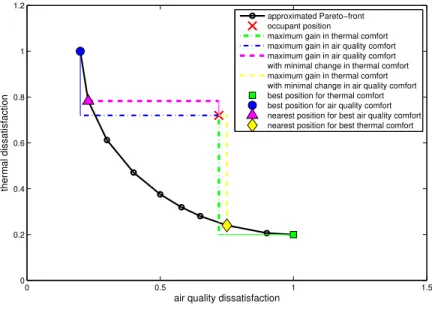
The set of trade-offs gives rise to a surface in the objective space which is popularly known as Front. In other words, for this work, the Pareto-Front is an approximated curve based on the optimization results when plotted as thermal dissatisfaction versus air quality dissatisfaction or vice-versa. From the recorded data, the thermal and air quality state can also be marked and hence, present the system state compared to optimal state in a graphical format as shown in Fig. 7. The system state depicts the aggregate result of a non-optimal scenario as it is played by the occupants and thus reflects the quality of their behavior.

Based on each criteria, several points on the approximated Pareto-front are selected and the occupant is presented with a set of four possibilities which are as follows:

1. The state of the house or the actions (opening/closing of doors/windows) that can be considered by the occupant for achieving minimum air quality dissatisfaction (or equivalently maximum air quality comfort) while suf-fering some losses on the thermal comfort. This is marked by a blue circle on Fig. 7.

2. Like the previous case, the actions that can be considered by the occupant for achieving maximum thermal comfort while suffering some losses on the air quality comfort. This is marked by a green square on Fig. 7.

3. The actions that can be considered by the occupant for obtaining max-imum improvement on the air quality comfort while sacrificing minimal amount of thermal comfort. This is marked by a magenta triangle on Fig. 7.

0 0.5 1 1.5 0 0.2 0.4 0.6 0.8 1 1.2

air quality dissatisfaction

thermal dissatisfaction

approximated Pareto−front occupant position

maximum gain in thermal comfort maximum gain in air quality comfort maximum gain in air quality comfort with minimal change in thermal comfort maximum gain in thermal comfort with minimal change in air quality comfort best position for thermal comfort best position for air quality comfort nearest position for best air quality comfort nearest position for best thermal comfort

Figure 7: Optimal scenario and consequences of occupant’s historical actions.

4. Like the previous case the actions that can be considered by the occupant for obtaining maximum improvement on the thermal comfort while sacri-ficing minimal amount of air quality comfort. This is marked by a yellow diamond on Fig. 7.

It is further emphasized that each of these vectors (black points) in the Pareto-front as shown in Fig. 7 corresponds to some scenario and thus, repre-sents a behavior of the occupant in terms of openings and closings of doors and windows over 12 hours on a particular day.

4.3

Multi-objective Differential Evolution

The goal is to provide the occupant with support to improve his behavior by understanding how far he is from optimal behavior. The optimal behavior is a set of solutions consisting each in a scenario of openings and closings . This optimization problem is addressed with the multi-objective version of differential evolution (DEMO) algorithm [10]. The algorithm is briefly described next. It consists of the following steps: initialization, mutation, recombination and selection.

4.3.1 Initialization

For the first generation, several numbers (20, for this work) of population candi-dates are randomly initialized where each candidate is a 24-dimensional vector

(A) whose each element is either open (1) or close (0) status of door or window. 4.3.2 Mutation

In this step, for every i-th candidate in the population, three candidates and random indices r1, r2and r3are chosen such that i, r1, r2 and r3are mutually

exclusive. The donor vectors, Vi,G, are generated at the mutation step for

generation G by Eq. (14) where F is called the scale factor which is randomly selected such that F ∈ [0, 2]. To ensure that the constituents of the vectors are binary, the floor function (b.c) has been employed.

Vi,G= Ar1,G+ bF × (Ar2,G− Ar3,G)c (14)

4.3.3 Recombination

The constituent of donor solutions and candidate solutions are chosen to con-struct the trial solutions, Ui,G, based on the crossover ratio, CR ∈ [0, 1] which

is a random value. Recombination follows Eq. (15) which suggests that higher value for CR favors selection of donor solutions and hence, CR was chosen to be 0.8. A random index Irand is selected for which the constituent of the donor

is considered so that the trial vector is always new.

uij,G=

(

vij,G, if randij ≤ CR or j = Irand

aij,G, if randij > CR and j 6= Irand

(15)

4.3.4 Selection

The fitness evaluation of a solution is dictated by Eq. (11). Since there are multiple criteria for selection, Pareto-dominance relation between the fitnesses of the trial and candidate solutions helps to decide which solution is chosen for the next generation. Selection is governed by Eq. (16) whereas Eq. (17) demonstrates Pareto-dominance relation [11] where A1Pareto-dominates A2i.e.

A1 A2. Since, the aim of this optimization problem is to increase the comfort

of the occupant, minimization of dissatisfaction defined in Eq. (12) and Eq. (13) are to be considered.

Ai,G+1=

(

Ai,G, if D(Ai,G)  D(Ui,G)

Ui,G, otherwise

(16)

∀i ∈ {1, 2}, di(A1) ≤ di(A2)

and ∃j ∈ {1, 2}, dj(A1) < dj(A2)

(17)

At the end of a large number of generations (300 for this work) by which the optimization is believed to have converged to some optima, a set of solu-tions and the associated set of criteria are obtained. At the termination of the optimization algorithm, the subset of solutions is selected such that no other

solution Pareto-dominates any solution of this subset. This subset is known as the Pareto-optimal set and the corresponding criteria forms a set known as Pareto-Front.

Pareto-Front represents the set of the optimal possible solutions that the occupant can take depending on his preferences. Based on this Pareto-Front, the suggestions illustrated in Fig. 7 are obtained. The assessment of the best candidate solution proceeds as follows. The city-block distance, as given by Eq. (18), (representing the net dissatisfaction) [12, 13] of every objective vector, Di,

from the reference objective vector, D0, is used as an indicator. The origin

(coordinate (0, 0)) of the objective space is considered as the reference objective vector because it is the minimum possible value either of the thermal or air qual-ity dissatisfaction can attain. Hence, this qualqual-ity indicator is used for ranking solutions at every generation of optimization and also for reporting the best can-didate solution after termination of the optimization algorithm. Best cancan-didate solution is that solution whose objective vector is closest to the origin of the ob-jective space. This obob-jective vector represents the best trade-off among all the conflicting objectives (considering equal preference of the different objectives) and its corresponding solution is the approximation of the optimal schedule of door and window opening/closing (A∗) that the occupant can consider. The indicator, given by Eq. (18), can also be used to measure the distance between the a Pareto-optimal solution and the user position by replacing D0 with the

dissatisfaction values obtained from the historical data.

Dist(Di, D0) = 2

X

k=1

|dik− d0k| (18)

To assess the problem at hand, the solution from the optimization problem obtained using the data of a random day from last year (i.e. recordings of 05/May/2015) is depicted in Fig. 8. The user position or the dissatisfaction on 05/May/2015 obtained from historical data is marked as a blue cross on Fig. 8. The solution corresponding to the nearest objective vector of the Pareto-Front from the origin is the best schedule proposed to the occupant. From the set of different solutions the four compromises of interest as mentioned in Section 4.2 are chosen. Based on this example, solutions 1 and 2 merges with solutions 3 and 4, respectively, and forms the end coordinates of the curve representing the Pareto-Front. Hence, two solutions at both the ends of the Pareto-front along with the solution nearest to the ideal objective vector (origin) are the schedules to be analyzed further. These proposed schedules along with the schedule of actions performed by the occupant results in a set of 12 temperatures and CO2

concentrations, which are shown in Fig. 9 and 10 respectively. The observations made from Fig. 8 is not so much evident for the occupant. However, from Fig. 9 and 10 the occupant can understand how much gain in thermal comfort can be achieved in different hours using the proposed optimal set of actions. Moreover, from this optimal set of actions the physical model can generate its associated state, which can be compared with the occupant’s state to generate the differential explanations and influences (explained in Section 5) and thus

present to the inhabitant the possible changes in actions to improve his comfort. 0.10 0.15 0.20 0.25 0.30 0.35 0.40 0.45 0.50

Thermal Dissatisfaction

Air

Q

ua

lity

Di

ssa

tisf

ac

tio

n

Several Possible States

Pareto-Front

User Position

Figure 8: Results from Multi-objective Differential Evolution for comparison with User Position

From these results, it can be observed that the usual schedule of actions followed by the occupants is worse with respect to all the three proposed sched-ules. Following any of the proposed schedules of actions will lead to decrease in the dissatisfaction with respect to both air quality and office temperature. This is consistent with both the temporal results (Fig. 9 and 10) and the resultant Pareto-Front (Fig. 8).

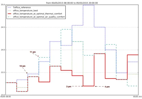
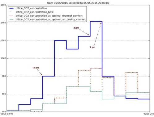
As an example scenario, the temperature and CO2 concentrations based on

the occupants behavior peaks between 3pm to 4pm as shown in Fig. 9 and 10. From Fig. 9, during 3pm to 4pm, it can be observed that if the scenario for optimal air quality is chosen, the temperature decreases but it decreases much more if the scenario for optimal thermal quality is chosen. Even at times like the period between 11am to 12pm in Fig. 9, reaching optimal air quality comfort can lead to increase in room temperature i.e. loss in thermal comfort.

Similarly, from Fig. 10, during 3pm to 4pm, it can be observed that if scenario for optimal thermal quality is chosen, the CO2 concentration in the

room decreases but it decreases much more if the scenario for optimal air quality is chosen.

With further analysis, it can be seen from Fig. 9 and 10 that for most of

Figure 9: Average office temperatures at different hours showing the proposed temperatures and the recorded temperatures

the hours, the curve corresponding to best schedule of actions (average dissatis-faction nearest to the origin) lies between the curves which originates from the end points of the Pareto-Front. This is not the case at the end hours of the day. However, it can be addressed to the fact that the minimization is performed on the average dissatisfaction measured across the entire day and not at every hour. Hence, using this proposed method optimal schedules can be generated for comparison with the historical schedule of the occupants.

Among the several schedules generated from the Pareto-front, based on the solutions discussed in Section 4.2, a few solutions are chosen for comparison. The user can prefer any of these schedules to compare his past schedule and learn the impact of his actions. The information on impact of his actions is generated using differential explanations as described in the next section. Thus, in order to compare his past actions, a single schedule has to be rendered. Considering equal preferences of the occupants with respect to thermal and air quality dissatisfaction, the schedule generated from the point on the Pareto-Front which is closest to the origin of the objective space (Eq. (18)) is presented for generating the differential explanations.

Based on these results, occupants can get an indicator of the amount of gain or loss in temperatures and CO2 concentrations to be achieved by them while

following the actions proposed by the system for the entire day. The differential explanations, explained in Section 5, will lead the occupants to understand what actions are to be taken to achieve these best comfort levels.

Figure 10: Average concentrations of CO2 at different hours showing the

pro-posed concentrations and the recorded concentrations

5

Differential Explanations and Influences

Differential explanations are constructed by analyzing the difference between two scenarios (the historical one and the optimal one calculated by the system) to assist the occupants to understand the impact and the effect of their daily actions on the optimality of their desired criteria.

From the optimization results, occupants can understand their position ac-cording the possible set of the optimal solutions for the entire day. Differential explanations will help them to understand how and what needs to be done to reach the chosen optimal solution according to their objectives.

This comparison includes the set of actions, the intermediate variables, and the effects. The variables are concerned with the consequences of the difference between the users’ actions and the optimal actions, and form the basis for the explanations. With this, it is possible to generate an indicator for the impact of those actions on the optimality. It also requires evaluation of the different criteria and represents them in the form of cause-effect relation to make them more clear for occupants.

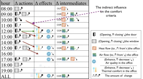
In Fig. 11, the differential explanations are illustrated in a table where the first column represents the distance of optimality for actions with what the occupant should have done according to the optimal plan, as shown in Eq. (19). A?_k− ˜Ak = ∆Ak (19)

where A?

k represent the action (Fig. 2) calculated by the optimizer at instant

k while ˜Ak represents a measured occupant’s action at the same instant. The

variable, k, can take any value in [0, 23]. In this paper, k = [8, 20] , ∀k, because it focuses on the time where occupants are present (daytime period). At 8am, for instance, the inhabitant should have opened the window more. At 4pm, the user behaves according to best scenario.

The second column presents the effects (Fig. 2), like in the thermal comfort and the air quality. This is given by Eq. (20).

E_k?− ˜Ek = ∆Ek (20)

where E?

k represent the calculated effect by system at instant k while ˜Ek

represents the measured effect. The right-hand-side of Eq. (19) and (20) denotes the difference in actions of the occupants and its resulting difference in the effect at the k-th instant, respectively.

To better represent the causality in the explanations and extract the knowl-edge from the system, the intermediate variables are added in the third column of Fig. 11. Those variables are extracted to render the knowledge from the system explicitly.

The last row labeled ALL represents the overall gain or loss in the com-fort criteria throughout the day. To generate a small summary and give the inhabitant an indicator to optimality in general, for the entire day.

When computing the differential explanation, it is necessary to transform quantitative variable values into qualitative ones for a better understanding

Figure 11: Differential explanations help the inhabitants to understand their actions like at 4pm, the user behaves correctly (its action was similar to the proposed optimal plan); at 12am, the inhabitant should have opened the door for much longer time, this would helped him getting a high improvement in his thermal comfort and slight enhancement in the air quality.

for the occupants and defines the qualitative distance. For instance, telling the occupant that closing the door at 2pm will cause a lot of decrease in the airflow and that he will obtain a significant decrease in the air quality level is easier to understand rather than telling that a difference in airflow of 30% will lead to a difference in CO2 concentration of 400 ppm. The transformation

from quantitative to qualitative here is done by dividing the value domain of a variable into 7 sub-domains (3 positive, 3 negative and 1 no-change levels). Those levels were chosen from the physical world according to their impact on the model and the occupant.

The levels for the variations in thermal dissatisfaction are given by: ΠT_{−0.25,−0.15,−0.05,0.05,0.15,0.25}(∆σ_Tk(Tin))

The levels for the variations in air quality dissatisfaction are given by: ΠCCO2

−0.2,−0.1,−0.05,0.05,0.1,0.2(∆σairk (Cin))

The levels for the variations in the opening of the door and the window are given by:

Πopening_{−0.7,−0.5,−0.2,0.2,0.5,0.7}(∆ζD)

Πopening_{−0.7,−0.5,−0.2,0.2,0.5,0.7}(∆ζw)

The arguments of each of these discretization functions is the difference of the measured quantity with the proposed optimal value of the quantity.

Except for the no-change level, where arrows are omitted, 1 to 3 arrows have been used to represent the associated sign of variation (arrows direction) and intensity (number of arrows). For instance, in Fig. 11, the logo of window with three adjacent upward arrows means that the occupant should have opened the window for a much longer period of time during the corresponding time period. As it can be seen, the differential explanations are much easier to understand than the analysis of the 11 plotted curves (Fig. 3 to 6) where the inhabitant has to correlate the different actions, effects and intermediate variables. With differential explanation, it is thus easy for an occupant to identify the actions that needs to be modified, monitor the difference gained with respect to different criteria while at the same time use the intermediate variables as elements of understanding.

The differential explanation is providing a list of behavior modifications (opens the door for a longer period, for instance) with the associated impact. However, there are two limitations with such a description.

First, there is not a direct link between an action modification and its im-pact. Buildings have inertia i.e. energy dynamically stored in their structure. This inertia causes a delay and has a smoothing effect on different changes in the building preventing a rapid degradation or augmentations in temperature. Inertia is also present in the room volume for the CO2 concentration. Thus,

occupant actions might have a delayed impact.

Figure 12: Differential Explanations with Influences

In Fig. 12, closing the door at 10am does not have an immediate impact but it has a strong influence on the air quality at 12pm: it is a calculated delayed impact.

impor-tance: some of them have a limited influence and could be skipped if necessary (the inhabitant might not want for instance to interrupt his current activity to close the window). But some of them should be followed because of their high influence on the selected criteria (like the previous door example having a strong influence on the air quality).

Lets consider

˜

A = { ˜Ai,k; ∀k}

A?= {A?_i,k; ∀k} (21) where i stands for the different actions (window and door) and k for the time period. The influence of each action is determined by changing one action at a time like in Eq. (22). In a specific instant the calculated action will be equal to the measured action.

A?_t = {A?_k; ∀k 6= t} ∪n ˜At

o

(22) The physical model is then used to re-simulate the effects.

Physical model: A?t =⇒ E ?

t (23)

By comparing the optimal scenario with a scenario calculated by replacing one optimal action by the action that has been really done, it is possible to evaluate the impact of occupants behaviors that they may have on the comfort level and how it is preventing them from reaching the optimal level. For instance, on Fig. 12, occupant might discover that opening the window for longer time requested by the system at 8:00 will not change much the air quality at 12:00 but not closing the door at 10:00am could dramatically change the level of the air quality at 12:00pm.

E_t?− E?

k = ∆E (24)

Thus, the proposed method allows the occupants to have an explanation based on the cause-effect relations of their actions and they may decide to change their routines, learning from their historical actions.

6

Conclusion

The main objective of this paper is to help the occupants to get a better un-derstanding of their energy management system and their actions. This work discusses and presents why explanations are needed and why they are important for occupants apprehension of the energy management system and the impact of their actions. It presents the concept of differential explanations i.e. a type of cause-effect explanations and also presents the concept of influence of the in-habitant’s actions to clarify for him/her the long term effect of his/her actions. This study uses the multi-objective version of differential evolution (DEMO) for

proposing optimal actions to the occupant based on his/her past actions. This is preliminary work dealing with thermal and air quality comfort criteria.

In future, this work will examine different methods to build and generate qualitative models to define causality between actions and their causal chain of impacts. This can be done by using causal physical models like bond graphs [14] and try to profit from the techniques of the causal graph to formalize the causal explanations like by using GARP3 [15] as workbench for qualitative reasoning and modeling.

Another aspect to be explored is the optimal schedule obtained when other criteria such as humidity, consumption of energy, price of electricity, etc. come into play. Besides having multiple criteria, the occupant may be biased towards certain criteria. Hence, the preference of the occupant plays a crucial role in decision making. Incorporating such user preferences is another open area of research. As the only machine learning tool used in this work is the optimization algorithm, the comparison of the performance of the proposed approach using other optimization algorithms is to be studied further.

Acknowledgment

This study has been supported by the Indian side of the project sanctioned vide DST-INRIA/ 2015-02/ BIDEE/ 0978 by the Indo-French Centre for the Promotion of Advanced Research (CEFIPRA —IFCPAR).

This work benefits from the support of the INVOLVED ANR-14-CE22-0020-01 project of the French National Research Agency [16] which aims at imple-menting new occupant interactive energy services, like MIRROR, WHAT-IF and SUGGEST, into a positive energy building constructed at Strasbourg in France by Elithis.

References

[1] E. of France EDF. (2016) Le btiment, premier poste de consommation dnergie en france. [Online]. Avail-able: https://www.lenergieenquestions.fr/le-batiment-premier-poste-de-consommation-denergie-en-france/

[2] B. Bredeweg and K. D. Forbus, “Qualitative Modeling in Education,” AI Magazine, vol. 24, no. 4, p. 35, Dec. 2003. [Online]. Available: http://www.aaai.org/ojs/index.php/aimagazine/article/view/1729

[3] F. C. Keil, “Explanation and Understanding,” Annual review of psychology, vol. 57, pp. 227–254, 2006. [Online]. Available: http://www.ncbi.nlm.nih.gov/pmc/articles/PMC3034737/

[4] F. Heider, The Psychology of Interpersonal Relations. Psychology Press, 1958.

[5] E. Sober, “Common Cause Explanation,” Philosophy of Science, vol. 51, no. 2, pp. 212–241, 1984.

[6] R. A. Wilson and F. Keil, “The Shadows and Shallows of Explanation,” Minds Mach., vol. 8, no. 1, pp. 137–159, Feb. 1998. [Online]. Available: http://dx.doi.org/10.1023/A:1008259020140

[7] S. P. Lisa SCANU, Pierre BERNAUD and E. WURTZ, “Mthodologie pour la comparaison de structures de modles simplifis.” France: IBPSA, 2016. [8] M. Amayri, S. Ploix, and S. Bandyopadhyay, “Estimating occupancy in an office setting,” in Sustainable Human Building Ecosystems, Carnegie Mellon University, Pittsburgh, USA, 2015, pp. 72–80.

[9] L. D. Ha, H. Joumaa, S. Ploix, and M. Jacomino, “An optimal approach for electrical management problem in dwelings,” Energy and Buildings, vol. 45, pp. 1–14, february 2012.

[10] T. Robiˇc and B. Filipiˇc, “Demo: Differential evolution for multiobjec-tive optimization,” in Evolutionary multi-criterion optimization. Springer, 2005, pp. 520–533.

[11] H. Ishibuchi, N. Tsukamoto, and Y. Nojima, “Evolutionary many-objective optimization: A short review.” in IEEE congress on evolutionary compu-tation, 2008, pp. 2419–2426.

[12] R. A. Melter, “Some characterizations of city block distance,” Pattern recognition letters, vol. 6, no. 4, pp. 235–240, 1987.

[13] R. M. de Souza and F. d. A. De Carvalho, “Clustering of interval data based on city–block distances,” Pattern Recognition Letters, vol. 25, no. 3, pp. 353–365, 2004.

[14] C. Ghiaus, “Fault diagnosis of air conditioning systems based on qualitative bond graph,” Energy and Buildings, vol. 30, no. 3, pp. 221 – 232, 1999. [Online]. Available: http://www.sciencedirect.com/science/article/pii/S037877889800070X [15] B. Bredeweg, A. Bouwer, J. Jellema, D. Bertels, F. F. Linnebank,

and J. Liem, “Garp3: A new workbench for qualitative reasoning and modelling,” in Proceedings of the 4th International Conference on Knowledge Capture, ser. K-CAP ’07. New York, NY, USA: ACM, 2007, pp. 183–184. [Online]. Available: http://doi.acm.org/10.1145/1298406.1298445 [16] A. A. N. de la recherche. (2015) Involved project. [Online]. Available:

http://www.agence-nationale-recherche.fr/?Projet=ANR-14-CE22-0020