CHD : a two-dimensional, multigroup, rectangular geometry, cubic hermite, finite element diffusion code

NUCLEAR

ENGINEERING

MITNE--181

READiNG

ROOM -

M.-CHD: A TWO-DIMENSIONAL, MULTIGROUP,

RECTANGULAR GEOMETRY, CUBIC HERMITE,

FINITE ELEMENT DIFFUSION CODE

by

F. A. Kautz

L.

0. Deppe

June 1975

DEPARTMENT OF NUCLEAR ENGINEERING

MASSACHUSETTS INSTITUTE OF TECHNOLOGY

Cambridge, Massachusetts 02139

AEC Research and Development Report

Contract AT(1 1-1)-2262

MASSACHUSETTS INSTITUTE OF TECHNOLOGY

DEPARTMENT OF NUCLEAR ENGINEERING Cambridge, Massachusetts 02139

CHD: _{A Two-dimensional, Multigroup,}

Rectangular Geometry, Cubic Hermite, Finite Element Diffusion Code

by F. A. Kautz L. 0. Deppe June 1975 COO--2262-10 MITNE--181

AEC Research and Development Report

Contract (11-1)2262

CONTENTS

Abstract

I. Introduction II. Theory

A. The Time-Independent Neutron Diffusion

Equation

B. Finite Element Methods and the Weak Formulation

C. The Weak Form of the Diffusion Equations D. Multigroup Diffusion Equations

1. Generalized Multigroup Equations

2. Conventional Multigroup Equations

E. Spatial Approximations

1. Construction of Basis Functions for

Piecewise Expansion in One Dimension 2. Construction of Basis Functions in

Two Dimensions

3. Varying Cross Sections within the

Expansion Element

4. Matrix Formulation of the Multigroup Diffusion Equations

F. Solution Algorithms

1. Boundary Conditions

a. Vacuum Boundary Condition

b. Zero Derviative Boundary Condition

2. Iterative Processes 1 4 6 6 10 13 16 16 17 19 20 32 45 47 54 54 54 55 55

3. Convergence Acceleration of the Outer

Iteration 57

4. Convergence Tests 59

III. Sample Problems and Results 60

A. The One-dimensional, Ten-region Problem 60

B. The Basic Two-dimensional, Two-composition

Problem 67

C. The Basic Two-dimensional Problem with a Baffle

Surrounding the Fuel Region 72

D. The Basic Two-dimensional Problem with Varying

Cross Sections within the Fuel Region 79

E. Results of IAEA 2-D Benchmark with Various

Coarse Meshes 88

F. Results for Maine Yankee in Two Dimensions

with Various Coarse Meshes 96

G. Results for Zion 1 in Two Dimensions with

Various Coarse Meshes 105

IV. A Guide to User Applications 113

A. Overall Program Flow 113

B. Details of Program Options 113

1. Cross Section 113

a. Input Formats 113

b. Cross Section Collapsing 116

2. Finite Element Expansion Function

Specification 117

3. Geometry and Boundary Condition

a. Spatial Mesh

b. Boundary Conditions

c. Specifications of Elements with either

Varying Cross Section or Constant Cross Section Subregions

4. Flux Input Options

5. Flux Dumps and Restart Procedures 6. Convergence Criterion Specifications 7. Edit Options

a. Element Edit

b. Zone Edit c. Point Edit

C. Description of Input Data 1. Job Title Card

2. Input of Control Numbers

3. Problem Dependent Data

4. Edit Input

V. Programming Information

A. Program Structure 1. Program Flow

2. Role and Function of Subprograms

3. Relation of Problem Variables and Program

Mnemonics

4. Definition of Important Variables in Common Blocks and Argument Lists B. Hardware Requirements C. Software Requirements D. Programming Considerations 120 122 123 125 125 127 128 128 128 130 131 131 131 135 140 143 143 143 143 143 149 149 149 154

1. Variable Dimensioning 154

2. Ordering of Unknowns 154

FIGURES

Figure 1. A Function f(x) and a Uniquely Determined

Interpolate si(x) in the Interval

(xi, xi+1).

Figure 2. One-dimensional Cubic Element Functions

Figure 3. Cubic Basis Functions Appropriate for

Functions and Derivative Continuity

Figure 4. Cubic Basis Functions Appropriate for Flux

and Current Continuity Across Interface

Figure 5a. Linear Element Functions

Figure Sb. Linear Basis Functions Appropriate for

Flux Continuity Across Interface

Figure 6. Hermite Interpolation Data in a Rectangular

Mesh

Figure 7. Bicubic Basis Functions

Figure 8. Basis Functions on Boundary Points of a

Rectangular Mesh

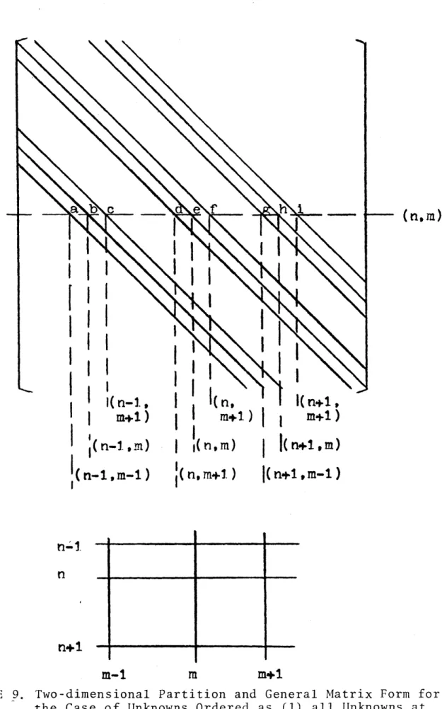
Figure 9. 'Two-dimensional Partition and General Matrix

Form for the Case of Unknowns Ordered as

(1) All Unknowns at Each Point, (2) All Mesh

Columns, and (3) All Mesh Rows

Figure 10. Two-dimensional Partition and Corresponding

Submatrix (e.g., Lg) Structure

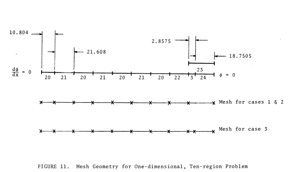
Figure 11. Mesh Geometry for One-dimensional,

Ten-region Problem 22 25 27 29 30 31 34 42 44 51 52 62

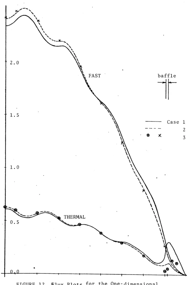
Figure 12. Figure 13. Figure 14a. Figure 14b. Figure 15. Figure 16a. Figure 16b. Figure 17. Figure 18a Figure 18b.

Flux Plots for the One-dimensional,

Ten-region Problem 65

The Basic Two-dimensions, Two-composition

Problem 68

Thermal Flux Plots for the Basic Two-Dimensional, Two-composition Problem at

x = 0.0 70

Thermal Flux Plots for the Basic Two-dimensional, Two-composition Problem at

x = 20.0 cm 71

Geometry for the Basic Two-dimensional Problem with Baffle Surrounding the Fuel

Region 73

Thermal Fluxes at y = 0.0 for the Basic

Two-dimensional Problem with a Baffle

Surround-ing the Fuel Region 76

Thermal Fluxes at y = 20.0 for the Basic

Two-dimensional Problem with a Baffle

Surround-ing the Fuel Region 77

Geometry for the Basic Two-dimensional Problem with Varying Cross Sections within

the Fuel Region 80

Thermal Fluxes at x = 0.0 for the Basic

Two-dimensional Problem with Varying Cross Sections

within the Fuel Region 83

Fast Fluxes at x = 0.0 for the Basic

Two-dimensional Problem with Varying Cross

Figure 19a. Thermal Fluxes at x = 20.0 cm for the

Basic Two-dimensional Problem with Varying

Cross Sections within the Fuel Region 85

Figure 19b. Fast Fluxes at x = 20.0 cm for the basic

Two-Dimensional Problem with Varying Cross Sections

within the Fuel Region 86

Figure 20. Core Layout for IAEA Benchmark 89

Figure 21. CHD 8 x 8 Mesh for IAEA Benchmarks 90

Figure 22. CHD 7 x 7 Mesh for IAEA Benchmark 91

Figure 23. Assembly Power Fraction Comparison for IAEA

Benchmark 92

Figure 24. Percent Error in Assembly Powers for IAEA

Benchmark 93

Figure 25. Comparison of Percent Error in Assembly

Powers with Cubic Hermite and Linear

Hermite Elements for IAEA Benchmark 95

Figure 26. Core Layout of Maine Yankee 97

Figure 27. CHD 11 x 11 Mesh for Maine Yankee 98

Figure 28. CHD 8 x 8 Mesh for Maine Yankee 99

Figure 29. CHD 7 x 7 Mesh for Maine Yankee 100

Figure 30. Assembly Power Fraction Comparison for

Maine Yankee 101

Figure 31. Percent Error in Assembly Power for Maine

Yankee 103

Figure 32. Core Layout for Zion 1 106

Figure 33. CHD 7 x 7 Mesh for Zion 1 107

Figure 35.

Figure 36.

Figure 37.

Figure 38.

Figure 39.

Assembly Power Fraction Comparison for Zion 1

Assembly-averaged-to-core-averaged Power Ratios for Zion 1

Simplified Logical Flow Diagram for CHD Coordinate System Orientation Assumed

by CHD

Program Subroutine Flow Chart for CHD

109

110

114

121

TABLES

Table I. Eigenvalues for the One-dimensional

Ten-region Problem 63

Table II. Element-averaged Results for the

One-dimensional, Ten-region Problem 64

Table III. Eigenvalues for the Basic

Two-Dimensional, Two-composition Problem 69

Table IV. Results for the Basic Two-Dimensional

Problem with a Baffle Surrounding the

Fuel Region 75

Table V. Some Results for the Basic

Two-Dimensional Problem with Varying Cross

Sections within the Fuel Region 82

Table VI. Data for IAEA 2-D Benchmark Analysis 94

Table VII. Data for Maine Yankee Analysis 104

Table VIII. Data for Zion 1 Analysis 112

Table IX. Description of Expansion Function Options 118

Table X. Default Expansion Function Sets 119

Table XI. Function of CHD Subroutines 145

Table XII. Relation of Some Problem Variables to

Program Mnemonics 148

Table XIII. Definitions of Some Important Program

Variables 150

REFERENCES

Appendix A: Macroscopic Cross Sections for Test Problems 158

Appendix B: Inner Products for Cubic Hermite Element

Functions

Appendix C: Sample Problem Input and Output

161 166

CHD: _{A TWO-DIMENSIONAL, MULTIGROUP,} RECTANGULAR GEOMETRY, CUBIC HERMITE,

FINITE ELEMENT DIFFUSION CODE

by F. A. Kautz L. 0. Deppe

ABSTRACT

1. Program Identification: CHD

2. Description of Function: CHD solves the two-dimensional

multigroup diffusion equation in planar geometries using a general rectangular mesh. Regular inhomogeneous (keff) problems subject to vacuum or reflective boundary con-ditions are solved.

3. Method of Solution: A finite element method in which the flux is assumed to be given by a cubic Hermite poly-nomial in each rectangle is used to solve the

accelerated by a Chebyshev Technique.

4. Restrictions: _{Variable dimensioning is used so that any}

combination of problem parameters leading to a container array less than MSIZE can be accomodated. On IBM ma-chines, where CHD uses a combination of single precision

(4 bytes per word) and double precision (8 bytes per word), MSIZE can be several hundred thousand words (in terms of 4-byte words).

5. Computers for which Program is Designed and Others on

which it is Operational: _{IBM 370/168, IBM 360/91, IBM}

360/195.

6. Running Time: A two-group, 81-element, kef calculation

for the two-dimensional, quarter core IAEA benchmark

problem requires about 2.3 minutes of IBM 370/168 time.

Running times vary almost linearly with the total number of unknowns.

7. Programming Language; CHD is written in FORTRAN-IV.

8. Unusual Features of the Program: Element regions can

encompass areas with varying cross sections, with these cross section variations accounted for through the inner products of the basis functions. Thus each element

region can include more than one core assembly, taking advantage of the high-order flux expansion. Flexible edit options, including dumps and restart capability, are provided.

9. Machine Requirements: _{The standard output (scratch)}

units and system input/output units provided with IBM

360-370 machines are sufficient. A relatively large

10. Authors: The authors of CHD are F. A. Kautz and L. 0. Deppe, of the Department of Nuclear Engineering, Bldg.

24-212, Massachusetts Institute of Technology, 77

Massa-chusetts Avenue, Cambridge, MA 02139. The individual

currently responsible for the program is F. A. Kautz.

11. References: Publications which are directly related to

the methods incorporated in CHD are the following: (a) Kang, C. M., and K. F. Hansen, Finite Element Methods for Space-time Reactor Analysis, Sc.D.

thesis, Report MIT-3903-5, MITNE-135, Massachusetts Institute of Technology, Cambridge, MA 02139,

November 1971.

(b) Deppe, L. 0., and K. F. Hansen, The Finite

Ele-ment Method Applied to Neutron Diffusion Problems, Nucl.E. thesis, Report COO-2262-1, MITNE-145,

Massachusetts Institute of Technology, Cambridge, MA 02139, February 1973.

12. Material Available: Source deck, test problems, results

of executed test problems, and this report are avail-able from the Department of Nuclear Engineering,

I. INTRODUCTION

CHD is a program for solving the two-dimensional,

multigroup neutron diffusion equations using a rectangular mesh. The unknown solutions are expanded as bicubic Hermite polynomials in a piecewise manner using the Galerkin method

to arrive at a discrete formulation. The resulting

equa-tions are uncoupled via the power iteration technique, and the group solutions are obtained by direct inversion (using Cholesky factorization) of the coefficient matrix.

The code solves the standard eigenvalue (lamda mode) problems, providing flexible edit options which include

dumps and restart capability. Vacuum and reflection

boun-dary conditions are admissible, consistent with any problem type.

CHD is written in Fortran IV using flexible

dimension-ing so that the size of all arrays is established at the execution of a particular problem; hence, core storage requirements are minimized. Particular features of CHD include:

1. arbitrary group-to-group downscattering,

2. arbitrary group-to-group fission sources,

3. vacuum and reflective boundary conditions on all

sides,

4. rectangular domains,

5. elements which can encompass areas having varying

cross sections,

7. flexible input options for basis functions

specifications,

8. Chebyshev convergence acceleration for outer

iterations,

9. flexible restart and edit options, including

reaction rate edits over subregions within element regions.

The next section of this report contains the theo-retical development of all the methods and approximations used in CHD. Section III contains sample problems and re-sults, Section IV is a guide to user application, and Sec-tion V contains programming informaSec-tion.

II. THEORY

In this section the energy and spatial variables of the diffusion equation are discretized to obtain a set of

linear algebraic equations. The time-independent neutron

diffusion equation is written and discussed in Section II.A.

A general discussion of finite element methods and the weak

formulation of a problem is presented in Section II.B.

Section II.C is devoted entirely to a discussion of the weak

form of the diffusion equations. The multigroup form of the

diffusion equations is presented in Section II.D. The

details of spatial approximations used in CHD are given in Section II.E. The solution of the linear algebraic system obtained by these approximations is discussed in Section II.F.

A. The Time-independent Neutron Diffusion Equation

In this section we introduce the energy-dependent, time-independent neutron diffusion equation and discuss

proper boundary conditions. The derivation of this equation

can be found in Davison [1], Henry [2], and elsewhere [3], [4].

For reactor problems the mathematical model of the physical problem is usually defined so that the solution parameters are at least piecewise continuous across the

subregion interface of the model. Consider, therefore, a

boundary 3M. We assume that 2 consists of contiguous open

subregions Q., Z=1, 2, ... , L, each of which is bounded by

a . Symbolically,

L

Q_ U i Q

Furthermore, let-E < E < E represent the continuous

mi- max

energy variable, and define E H (Emin, E ).

Then, within any region Q , the continuous energy,

time-independent neutron diffusion equation can be written as

T D= - V -D(r, E) V_(r, E) + E t (r,E) D(r,E)

- f dEZ s(r,E'+E)#(r,E') - X(E)f dE'vEf(;E')4(rE'),

= Q(rE),

where

2

( (r,E) _{= scalar neutron flux (n/cm -sec),}

D(r,E) = neutron diffusion coefficient (cm),

Et (r,E) = total macroscopic removal cross section

(cm~ _), E a(r,E) E (r,E'+E) Zf(r,E) V vEf(r. E) E

Et(r,E) E Za(r,E) + maEs(r,E+E')dE',

min

= macroscopic absorption cross section (cm ),

= macroscopic scattering cross section

from E' to E (cm ),

= macroscopic fission cross section (cm ),

= average number of neutrons produced per

fission

= macroscopic fission neutron production

X(E) = fission spectrum for prompt neutrons,

= l/keff, eigenvalue introduced to define

an eigenvalue problem,

k eff = system multiplication factor,

Q(r,E) = extraneous source.

D, E a' s _{and Ef are continuous in each Q., Z=1, 2, ..}

L, and may be discontinuous on 3. If Q(r,E) = 0, then Eq.

(1) becomes an eigenvalue problem.

Eq. (1) is the result of a balance condition applied to

a volume element dr about r and to an energy interval dE about E. The first two terms on the left side of Eq. (1) account for the loses by net leakage and removal. The next two terms account for gains by inscattering from other

energies or by fissions at any energy,

We will impose any of the following homogeneous boun-dary conditions:

@(r,E) = 0

EE:

or for (2)

-5(r,E) =

0,

where 3/3n is the outward normal derivative at M.

The diffusion approximation fails in the neighborhood of material interfaces, where the solution has transients. We assume that the solution satisfies certain boundary

conditions at the interfaces. Rigorous interface boundary

transport theory are discussed in Davidson [1]. However, the following set of interface boundary conditions is more commonly used:

(r,E) = $(r+,E),

Ec

for

rs3Q

D(r~,E) $(r ,E) = D(r ,E)y-(r E). (3)

The negative and positive superscripts refer to opposite sides

of material interfaces. These conditions are the flux and

B. Finite Element Methods and the Weak Formulation

The finite element method consists basically of finding approximate solutions to Eq. (1) which are defined only over subregions (or finite elements) of the problem domain. When joined together, these piecewise solutions form an

approx-imate solution over the whole problem domain.

To generate these approximate solutions to Eq. (1) we

shall expand $ in terms of some suitable basis functions.

However, if we require the basis functions to have the same

differentiability properties and continuity properties as $

itself, then we will have great difficulties finding the

basis functions. _{In order to avoid these difficulties, we}

consider another formulation of the problem which weakens the continuity conditions and permits the use of a much broader class of expansion functions. We will now proceed to illustrate this "weak" formulation of a problem.

Consider the problem defined by

-V24(r)

where L is a linear operator with homogeneous boundary conditions

$(r) = 0

or for re 30

-$(r) = 0 (4b)

and continuity conditions

for re3O

Q(r) represents a source term.

This boundary-value problem can be cast in a varia-tional form. Given the funcvaria-tional

J = (L$,$) -2 (Q,$),

the condition under which J is stationary is given by

(Lp,u) - (Qu) = 0,

for all u in the same function space as

p.

for instance, denotes an inner product defined by

(Qu) =f2Qudv.

Integtating Eq. (6) by parts yields

(Vq,Vu) -f ( $. )udS - (Q,u) = 0.

DZ

(5)

(6)

(7)

Since homogeneous boundary conditions and derivative continuity conditions have been imposed, we see that the surface integral vanishes and we are left with

(V$,Vu) - (Qu) = 0. (8)

Eq. (8) is called the weak form of Eq. (6), and any $(r)

which satisfies Eq. (8) is called a weak solution to the

problem defined by Eqs. (4a, b, c). We observe that any $(r)

which is a solution of Eqs. (4a, b, c) is also a solution of

Eq. (8), and conversely, if the weak solution is in the

domain of the operator L, that is, twice differentiable in each R., then it also satisfies Eqs. (4a, c).

In order to approximate the solution to Eqs. (4a, b, c), we choose a convenient trial function space where the

piecewise functions {ui(r)}If ₁ form a basis. In particular,

we choose u (r) as polynomials of a certain degree satis-fying the same boundary conditions as the analytic solution.

We then seek an approximate solution of the form

M

() = . au (r) ₍₉₎

i=l 1

In the well-known Galerkin method [5], [6] of solving integro-differential equations, the expansion coefficients a are determined from the condition that the equation

obtained by the substitution of $(r) for $ in Eq. (4) must

be orthogonal to the elements u₁ , u₂, ... , uM. This

con-dition leads to the system of equations

(L$,u.) = (Q,u.), ₍₁₀₎

for all i = 1, 2, ... , M.

There are severe limitations to this particular

formu-lation. _{The expansion functions are required to be twice}

differentiable, and the interface continuity conditions are

imposed on the approximate solution. In view of the less

restrictive conditions on $ in the weak form of the problem,

we should expect that the class of appropriate expansion (or

basis) functions is much larger. $ is only required to be

piecewise continuous and may not satisfy the derivative continuity condition which appears as a natural interface

condition. These allow piecewise linear functions to be an

acceptable expansion functions in the weak form. Thus, in order to increase our degree of freedom in choosing expan-sion functions, we seek approximate solutions to the weak formulation of the problem, Eq. (8).

The Galerkin method then requires

(V$,Vu ) = (Q,u ) (11)

C. The Weak Form of the Diffusion Equations

Using the inner product for the space energy problem,

($,u)

f

we define the form (T$,u) as

(T$,u) - (VDV$,u) _{+ (E t} ,u)

-

(fdE'Es

1

- (X(E) fdE'vE f(E')$(E'),u).

In order for the terms of (T$,u) to exist, we must require

that $ and u be continuous and that $ have second

deriva-tives which are square intergrable.

The original (i.e., "rigorous") formulation of the diffusion problem may be stated as a problem of finding

$ in the domain of the operator T satisfying

(T$,u) = (Q,u). (12)

Intetrating the leakage term by parts, we obtain

XfdV(V-DV$,u) = (DV,Vu)

faJdS(Da ,u) , (13)

where the last term on the right is the sum of the surface

integrals for each subregion P of 0. Since $ satisfies

Eqs. (4b, c), the summation vanishes. Thus, Eq. (12) leads

to the weak form

where a($,u) is a bilinear form defined by

a($,u) = (DV$,Vu) + (Et$,u)

- dE'Es(E'+ -E)$ (E')u)

-

(X(E)f

Observe that in order for the terms of a($,u) to exist, we

require that $ and u be continuous and have first derivatives

which are square integrable. We define W1 _{(Q) (generally}

called a Sobolev space) as the set of all functions which

satisfy the above conditions. In view of the boundary

conditions in Eq. (4c), we shall use a subspace of W

(sM,

denoted by W (Q), whose elements satisfy the boundary

con-ditions stated by Eq. (4b).

The weak formulation of the diffusion problem may be

stated, therefore, as a problem of finding $ in W1 (Q)

satisfying Eq. (14), for all u in the function space W ₀ (Q).

Any $(r,E) which satisfies Eq. (14) is called a weak solu-tion to the diffusion problem.

It has been demonstrated by the steps leading from Eq. (12) to Eq. (14) that any $(r,E) which is a solution of Eqs.

(4a, b, c) is also a solution of Eq. (14). It can be shown

[7], conversely, that if the weak solution is twice

dif-ferentiable in each Q (i.e., in the domain of the operator

T), then it also satisfies Eqs. (4a,c). In particular, it

can be shown that the continuity conditions for D $

(cur-rent) in Eqs. (4a, c) are Euler equations in the varia-tion of u in the weak formulavaria-tion. For this reason, the

current continuity condition is called the "natural interface condition."

In the weak form of the diffusion equation, $ is only

required to be an element of the function space W1(2) and need not satisfy the current continuity condition which appears as

a natural interface condition. This allows the piecewise

linear function to be an acceptable function in the weak form. In fact, the weak form is very well suited for the use of piecewise polynomials as basis functions.

D. Multigroup Diffusion Equations

In Sections D and E, we briefly develop approximate methods for the solution of the weak form of the neutron

diffusion equations, Eq. (14). In this section, we consider

approximations of Eqs. (4a, b, c) in energy. The general-ized multigroup equations will be developed first, because of their relationship to formal few group theory [2], and then the conventional multigroup equations will be extracted from these generalized equations as a special case.

1. Generalized Multigroup Equations

We consider expansions of the flux in terms of piece-wise polynomials in both space and energy. The approximate

solution $(r,E) can be represented as

G M

$(r ,E) = ' X a. u.(r)u (E), (15)

g=1 i=l

where u (r) and u (E) are spatially dependent and energy dependent basis functions, respectively. The construction of these basis functions is discussed in Section E, and [7] presents further details.

We define the group flux approximation $ (r) as

M

9g = . _{=1ig 1 -}la. u.(r). (16)

Eq. (15) can then be written as

G

$(r,E) = I $ (r)u (E). (17)

-We apply the Galerkin scheme to Eqs. (4a, b, c), such that qsatisfies, for g=l, 2, ... , G,

(T$u) =(Q,u ) , ₍₁₈

($| ,u ) 0, (18

($,u ) and (DV$,u ) continuous on the material interfaces. _(18c)

where (ou)jf _{DudE. Eqs. (18a, b, c) lead to the generalized multigroup}

equations which are given by, for g=l, 2, ... , G,

G

- = V-D ,7 ,(r) =

with boundary conditions

g (r)| G X tgg' sg~ Vfg'9rg' Q g(r), g'1=1 tgg, sgg'X gg9 = 0, (19a) (19b) (19c) G

I(r), D ,(r) continuous at material interfaces

g g'=1

gg13g-where

D '9 (r) = (Du 9, (E),u 9(E)) ,

tgg 'E t(u , 1(E) u g(E))

sgg, ()= (fdE'Es (E'+E)u , (E'), u (E))

X = (X(E), ug (E)) ,

(fg = f dE'Ef(E'), u , (E')

Q (r) = (Q(rE), u (E))

g 9

2. Conventional Multigroup Equations

The conventional multigroup equations [1], [3], [4] are

obtained as a special case of Eqs. (19a, b, c). In this

a)

case, we specify

S(E), Eg>E>Eg+l

u (E) =

0, otherwise

where S(E) represents an infinite medium neutron spectrum. We then obtain the conventional multigroup equation, for g=1,

2,

G

X

-V-D VgY (r) + E t ) (r) - {z ,D + -v, =

Q

- g- g tg g - sgg g' x fg' g g

with boundary conditions

(r)| = 0, (20b)

g

-

3

(r) and D -4) (r) continuous at material interfaces, (20c)

where

D = 6 ,D g,

g gg g ,

tg ~gg'Z t

E. Spatial Approximations

The central problem in the application of the finite element method is finding appropriate piecewise continuous functions in an appropriate trial space (e.g., Hermite space or spline space) for use as trial functions in the approx-imate solutions to the convential multigroup equations,

M

= a. u.(r). (16)

g ig=' 1

-Polynomials are a natural choice for the basis functions

ui(r). They are easily integrated and differentiated, they

are well known, and they can be made complete. Other trial functions, such as trigonometric functions, can also be used.

Among the possible polynomial spaces, those based upon Lagrange and Hermite polynomials have been most widely

applied to diffusion problems. Lagrange polynomials are generated by using the function values at interval points of

the subregions. Hermite polynomials, on the other hand, are

generated through the use of values of the function and its

derivatives at the boundary of the subregions. In

partic-ular, the same data must be available at both ends of the interpolation interval. This means, for instance, that if one has the value of the function and its first order

deriv-atives at one end (or corner) of the interval, one must also have the value of the function and its first order

deriva-tives at the other end (or corners). Thus, the amount of

data is always an even number of values; hence the poly-nomials are always of odd degree. For neutron diffusion

problems, a desirable feature of Hermite polynomials is the fact that they allow the natural imposition of flux and current continuity conditions.

In the next two subsections of section E, we will sum-marize the construction of a complete basis for the piece-wise expansion of the solution to the weak form of the multigroup neutron diffusion equations, in one and two

dimensions, and in terms of the Hermite polynomials of the first and third degrees. The third subsection deals with varying cross sections inside the expansion elements, and the fourth subsection discusses the application of the

Galerkin technique to the weak form of the multigroup equa-tions and the matrix formulation of the problem.

1. Construction of Basis Functions for Piecewise Expansion

in One Dimension

We will now examine construction of the cubic Hermite basis functions appropriate for the expansion of the unknown solution in a one-dimensional space and indicate afterwards

the use of linear basis functions. In the next section, we

will consider the extension to two dimensions.

Consider a one-dimensional closed interval Q=[a,b] with a partition A of 0 such that

A:a=x <x2 ''''M = b, (21)

where A = (xi, xi+), i=1, 2, ... , M-1 are open subintervals

sufficiently smooth function f(x) in [xi, x i+], illustrated

in Fig. 1. When the values of both the function and its

first derivative at x and x i+1 are known, we consider the

use of polynomials si(x), of degree 2m-1 (where m=2 for the cubic interpolate) such that si(x) satisfies

S (P) (x.) = f (P (x.)

s i(p)

(22a)

(22b)

where s. ₁ (x.) _(x.)11 = -s.(x).

x

This type of interpolation

is called Hermite interpolation and it is known [8] that Hermite interpolate si(x) can be uniquely determined.

The Hermite interpolate si(x) of f(x) can be expressed a general way by

s (x) = m1 f(P)(x +)uP+(x) + f(P)(xi+l)up+1 (xI,

p=0

where the functions {uP±}, for m>1, are known as element

1

functions (i.e., piecewise polynomial functions) and are defined by 2m-1 1 _x, I a x ,x _- <x x , up(x) ₌ 1 J+

(x)

S. (x)

function and

derivative

values known _-derivative

values known

f(x)

a x ₁ xi+ 1 b

xD

FIGURE 1. A Function f(x) and a Uniquely Determined Cubic Interpolate S. (x) in the Interval [xi, x=l]

such that

uP xi)= 6. .6

0<pm-g1 j ij pg <p<m-l,

dx J P9'

where x.=x ±0. _{Note that u (x) and uP (}

j= i1 1+(x)are nonvanishing

over the same interval _{[x ,xi+i}

For the cubic Hermite interpolate (m=2), we have

s.(x) = f(x.)u +(x) + f(x _{)u + (x)u 1+}

+ f(l) (xi ₁)uK(x)

(25)

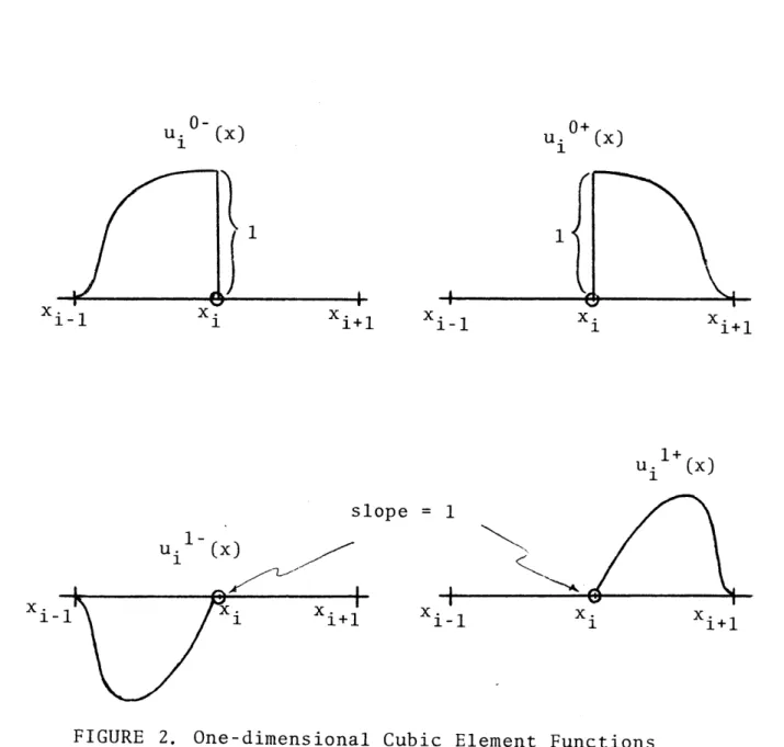
where the cubic element functions are

0-u (x) = 3 -- 2 X i 3 -0,1 x x<x, (26a) otherwise, 2 3 -i14 ( i+1~I i) 2x 2( _1-x -2 i+1~ _if 0, 3 > li <X x i+l' otherwise, 1 -u. (x)= _ i-1 2

i-l-x i-x x -xi i i-1P

x <ix<xi otherwise, 0+ u.(x (26b) (26c) 0,9

2 3 ________i) I i+1 i

(x i+; x ) x i-Xj 1-x - i+1

1+

ui +X (26d)

0, otherwise.

These element functions are illustrated in Fig. 2.

The error bound of the general Hermite interpolation is

stated by well-known theorems in [9], [10]. Within the %

interval [xi, xi+₁ ], the pointwise interpolation error for

one-dimensional neutron diffusion problems is bounded by

I

d 1 L(Ar)

where p=2m for this case and K is a positive constant

inde-pendent of jxi+1 --xil. The above expression states that the

bound in the pointwise error between f(x) and s(x) for a

piece-wise continuous function f(x) is of order 2m. Thus, for

the cubic Hermite interpolation (m=2), the error is

4

I

of O(Ax 4). For the linear Hermite interpolation (m=1),

the error is

SIf(x)-s (x) II <KI i(+ ₁~x)i 2

or O(Ax 2). The pointwise error in the derivatives is also

bounded with an appropriately lower exponent.

Now we consider the interval [a,b] partitioned into (M-1) contiguous subintervals. We can approximate the unknown so-lution of a problem over the whole interval by a sum of piecewise approximations, using a set of element functions

u 0-(X) xi 1 x1+1 _xi-i1 slope = 1 1-u. (x) i xi+1 xi-i

FIGURE 2. One-dimensional Cubic Element Functions

u 0+ xi-1 1 xi I-Xi+1 1+() xi-1 u X i Xi+1

7

1

in each subinterval, {uf , u'*, up-: 2<i<M-1, o<p<m-1}. Thus,

s(x) incorporating cubic Hermite element functions can be rep-resented by M-1 s(x) = [ s.(x) i= 1 M-i 1 ( )-I 1 0 (x+)up+x ()+f(P (x.)u+1(x)} M-1 + 0+ - 0 ()+ 1+

{f(x+)u. (x) if(x+₁ )ui+1(x) + f (+)ju((x)

i(1)

1-+ ( (x )u (x)}, (27)

where s (x) represents the Hermite interpolate in the element

A., defined by Eq. (23). The f's are unknowns to be

deter-mined.

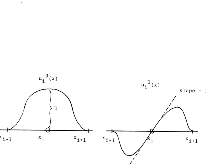
Function and derivative continuity can be naturally preserved by requiring

f(x+) = f(x.) = f(x.)

2_{<i<M-1 (28)}

f ( ( x ) - f ( ( x - f (1)(x i)

The conditions (28) lead to generation of the basis func-tions appropriate for the approximation of an unknown solution inside the interval [a,b], preserving function and derivative continuity across the interfaces. These coupled basis

func-tions are illustrated in Fig. 3.

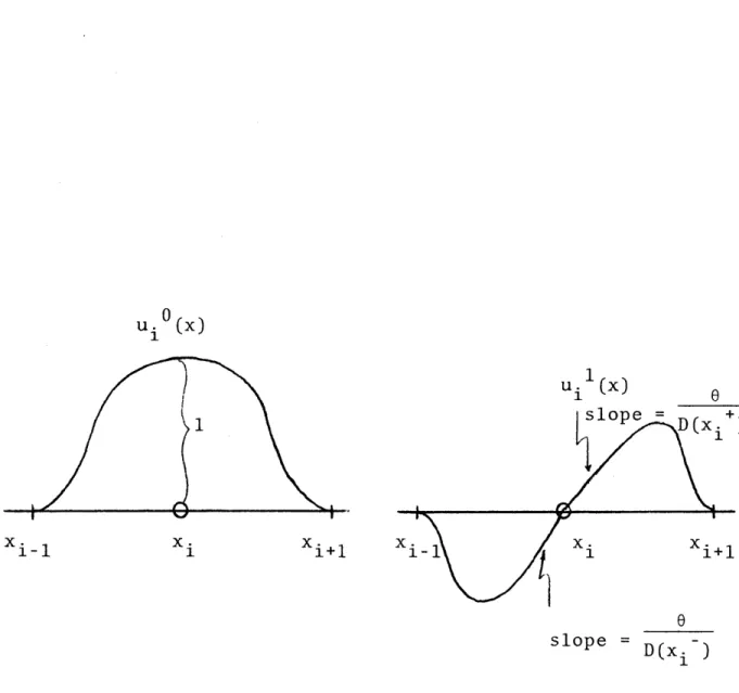
For neutron diffusion problems, however, we want to re-quire current continuity across the partition interfaces. This condition can be met if the 1-type (first derivative) basis functions are redefined in the following manner:

i

u. (x)

i

slope = 1

xi+₁

FIGURE 3. Cubic Basis Functions Appropriate for Function and Derivative Continuity 0

u. (x)

1

xi-1 xi

o u (x x, D(xi) u.(x) = (29)

o

where 0 is a normalization constant and uJ (x) are given by

Eqs. (26c, d). The normalization constant 0 is introduced in

order to produce stiffness matrices having small condition

numbers [7]. We usually choose 0 such that D ~ 1. These

D(x.) modified basis functions are illustrated in Fig. 4.

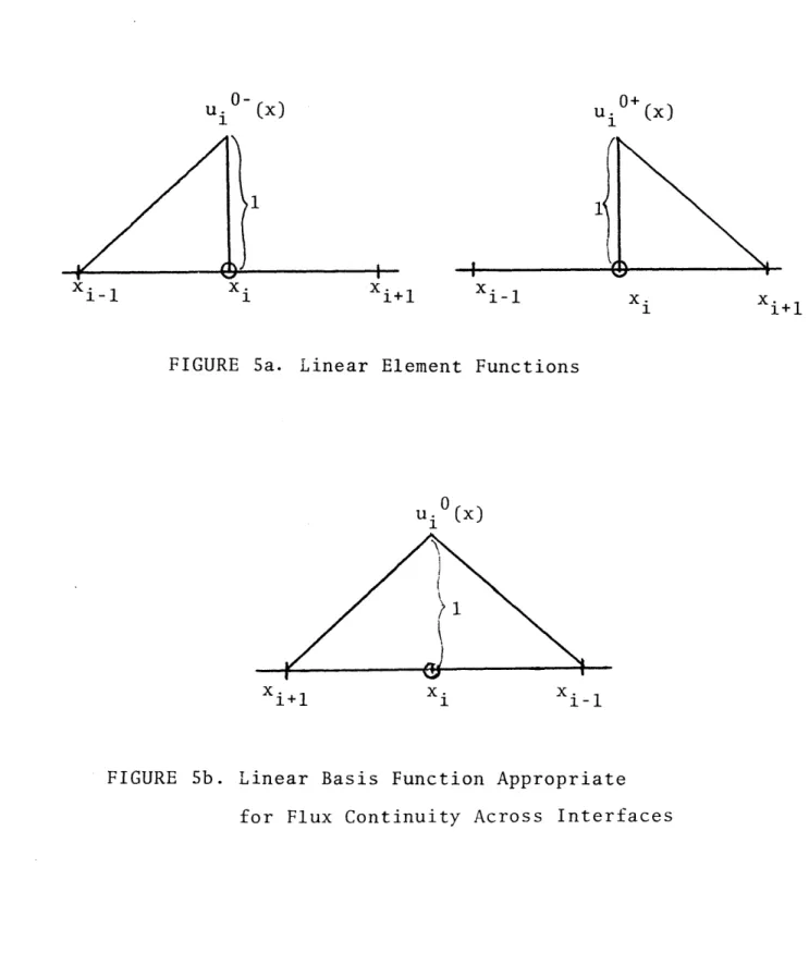
If piecewise linear element functions are used, we will be able to preserve only function continuity across the

par-tition interfaces. The element functions, illustrated in Fig. 5a, are represented by

x-x. x i - li-1 i u. (x) = (30a) 0 , otherwise, Xi+l- _{x <} 0+ u (x) = (30b) 0 , otherwise,

When the p oper coupling conditions (functions con-tinuity) are imposed, we will have defined the basis func-tions for the expansion, as illustrated in Fig. 5b.

u 0

uu _(x)

slope = (x

i-1 _{i i+1 i-1}

xi x.i

16

slope _D(x.)

FIGURE 4. Cubic Basis Functions Appropriate for Flux

and Current Continuity Across Interfaces x

.1

u. (x) _u 0+

1

K

x .

1 xi+l x x

FIGURE 5a. Linear Element Functions

u0

xi+l _{xi xi-l}

FIGURE 5b. Linear Basis Function Appropriate for Flux Continuity Across Interfaces

xi-₁

xi+l

It can be shown [7] that for the Hermite interpolate

s(x) [given by Eq. (27)] of the function satisfying the weak

form of the diffusion problem, the error bounds are

(f (x) - s (x)

)<K~x(mq

dx q LO [a, b]

where Ax = max Ix i+l-xi and K is a constant independent

l<i<M-1

of Ax. Thus, for the linear Hermite interpolation (m=l), the error in the function approximation is

2

II(f(x)-s(x))

L '[a,b] 2

or O(Ax ). For the cubic Hermite interpolation (m=2), the

error is 4 II (f(x)-s(x))||I <K2 Ax L'[a,b] 4 or O(Ax ).

2. Construction of Basis Functions in Two Dimensions

We now consider a two-dimensional region Q=[a,b]x[c,d] and assume an orthogonal coordinate system. Using Cartesian

coordinates, we define Tr to be a partition of Q such that

7T: a=x 1<x 2<- -<xM = b

(31)

c=y <y2< ...<yN = d.

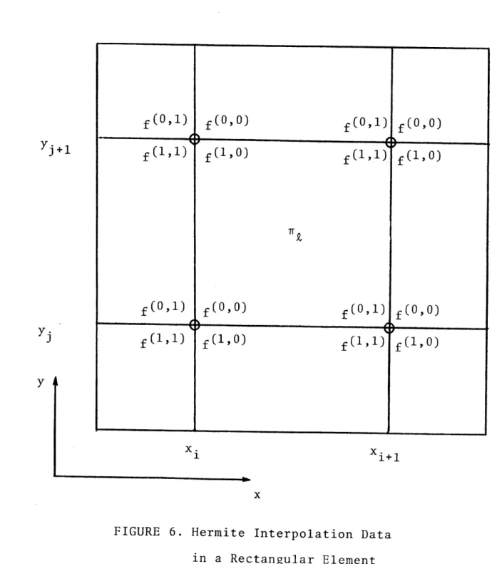
The set of all mesh points generated by 7 will be denoted Z,.

aenoted f., for k 2 1, 2, ... , L, with L = (M - 1) x (N - 1).

Each element 'rr has a set Z of 4 mesh points, namely the

corners of the mesh element. (See Fig. 6.)

The element functions in two dimensions are generated

by taking products of the one-dimensional element functions

in each direction. For instance, the two-dimensional

bi-cubic Hermite interpolate s,(x,y) in a mesh element 7r (see

Fig. 6) can be represented by

s (x,y) = f upx+(x)upy+(y) + p =0 p =0 i'Ti xy + fpx uX (x)u (y) + (i+1, i) (ExP) Ex+ p -+ f(XY) u, (x)u ( + 1 j+1) + f yj+1 u x )u (y) , (32)

where the subscripts (x ,y ) on f denote a value of the

function or its derivative at mesh point (i,j), and the

superscripts (pxp y'denote the p th derivative in the

x-direction and the py th derivative in the y-direction. Note that there are 16 coefficients (i.e., values of f) required to

specify a unique s (x,y). For this Hermite interpolation,

the interpolation data required to specify s,(x,y) are the

function values at the 4 mesh points of the element 7 ., the

first derivative in each direction at the 4 mesh points, and 2

the 4 mixed derivatives at each mesh point, i.e., at

each corner. Thus we have 4 values, 4 derivatives in x, 4

Yj+1

f(1,1)

f(1,o0)

(1,1

FIGURE 6. Hermite Interpolation Data

Hermite data are illustrated in Fig. 6.

The uniqueness and the approximation error for the Hermite interpolation are stated by theorems (with proofs)

in [7]. _{It is shown that a two-dimensional polynomial}

interpolate s ,(x,y), incorporating sufficiently smooth func-tions, satisfies the following expression for the pointwise error bound:

(f(x,y)-s ,(x,y))| <KAx(2mx-px) +

o ~x y L ( + K A (2my-py) y y (33) for 0Op <m -,

O<p

where K and K are positive constants independent of Ax

and Ay, respectively, and where (2_{mx -1) and (2m Y-1) specify}

the degree of the one-dimensional polynomials in each

direc-tion. Consequently, for the case of bilinear and bicubic

Hermite interpolation we have the following pointwise inter-polation error bounds:

j~~xy)s(xy)~2 2

f(xy)-s (xy)| L(7) <K Ax + K Ay (linear)

<K Ax + K Ay (cubic)

i.e., O(Ax2) + O(Ay2) for the linear and O(Ax 4) + O(Ay 4) for

the cubic interpolation.

In the region [a,b] x [c,d] partitioned into (M-1) x (N-1) contiguous subregions (or elements), we can approximate the

unknown solution of the problem over the whole region by a sum of piecewise approximations, using a set of element

(p , y)

functions in each mesh element, {u..

7

-O<p <m -l, -O<p <m -l}. Thus, the interpolate s(x,y)

incorporating bicubic Hermite element functions can be repre-sented by

L

s(x,y) = I st(x,y)

Z=1

N-1 M-1 1 (p ,p ) p +xp[ (y) +

j=i

x _y

+ f x'y0 u +(x)u y (y) +

(xi+1 '7

+fp P up x+ (XUp +

+f xEy91 (x)u. (y) +

(x ,yj +)

+ f x'E y u P+(x)u p (y) , (34)

(i+1'7j+13 i l ~

where s (x,y) represents the Hermite interpolate in the element ff

As in the one-dimensional case, basis functions for two-dimensional neutron diffusion problems can be defined

by imposing appropriate coupling conditions on the element

functions. The unknown solution of a two-dimensional problem

can then be approximated by considering a convenient partition of the problem domain.

First we consider the use of bilinear element functions. In this case there is one basis function at each mesh point which is defined by

0+ 0+ u. (x)u. (y), I 1 j 0- 0+ (0,0) u. (x)u. (y), II u (x,y) = 1 J 0-

0-u (x)u (y), III ₍₃₅₎

0+

0-u (x)u (y), IV

where the roman numerals refer to spatial mesh elements

sur-rounding point (ij) (as shown in Fig. 7). The piecewise

linear functions u. 0>x) 0 (y) are defined by Eq. (30).

1 J

up0,0)(x,y) is continuous; however, it does not satisfy the

continuity of D -1.

Next, we consider the construction of bicubic basis

functions from cubic element functions. These basis

func-tions depend on the diffusion coefficients surrounding a point (ij). Thus we consider two cases separately.

Case 1. DID III= D₁ IDiV

This condition is satisfied for any interior mesh

points or interface points except the singular points. The

proper basis functions are given by (see Fig. 7):

0+ 0+

u. (x)u (y), I

0- 0+

u. (x)u. (y), II

u(0,0) (xy) = (36a)

1J _0-

0-u. (x)0-u. (y), III

1 J1

0+

0-u. (x)0-u. (y), IV

u(1, _{U. 0)(xy)(xy} (x)u _{(xu ()}0+ 6 1-u I 1-(x ou 1+ DwIui

(

x)u0- _xi.()

_(y)

I II (36b) III IV or _{and y}

III ma be replaced by D 0_IV and D_III respectively.

u (0,1),y)_(xi) 0 0+ D-U-II 1+ (x)u. (y) , (x)u. (y) 3 0 _{u0 (x)u1 (y),} I I2 6 1+

III (x)u ₂₁(y), I (36c) III IV or D and D may u ij (x,y) = be replaced by a I 01+ 1+

nU. (x)u. (y),

DI 121 u ( D u x)u. (y) (x)u. 21 and D respectively. IV I II (y), III 0 1+ 1 -- U (X)u.j (y), IV (36d)

6 denotes a normalization constant and is generally taken

such that -~l. _D u(x), u(y), p=O, 1, are cubic element

13

functions defined by Eq. (26). The basis functions satisfy

the interface conditions of neutron flux and current contin-uity.

Case 2. DID III/ _{D ID I}

In this case, point (ij) is a singular point. It is well known that the diffusion approximation fails in the neighborhood of material interfaces, where the solution has transients. We do not expect analytic solutions near singu-larities to truly represent the physical neutron distri-bution. Furthermore, from a practical point of view, in many problems one is more interested in overall measures of

core performance (e.g., keff- reaction rates in assemblies

or larger regions). _{In these cases one may argue that,}

whatever the analytic singular component of the solution, it is a localized effect and its contribution to the overall results should be very small.

In calculations of realistic two-dimensional problems, on the other hand, one will have some pattern of zones with different fuel enrichments throughout the core, so that many

of the actual mesh points will be singular points. We

expect the singularity to be a function of the magnitude of the material discontinuities. A singularity will have a

greater influence at water-fuel interfaces than at interfaces between fuels of different enrichments.

singular points in problems where one is primarily concerned with region-averaged quantities (e.g., reaction rates for

depletion analysis). For instance, when DID III/ D ID y it

is easy to show that the interface conditions of current continuity permits P(x,y) to have only

-D(x)Y) (i,j) " (xY) I (i,

j)

Therefore, in Eq. (36), u 0? 1)(x,y) and u '0 (x,y) could be eliminated, leaving the proper basis functions to consist of two functions

u(0,0)(x,y); Eq. (36a),

(37) u .' (x,y); Eq. (36d).

1J

However, since the analytic solution at singular points is

not necessarily required to satisfy 4-4(xy) 1 c(xy) =0

the use of the basis functions defined by Eq. (37) can distort the solution and can lead to poor approximations, especially for coarse mesh calculations.

Another approach would consist of arbitrarily speci-fying first derivative continuity by making all coefficients

= 1 in Eq. (36). This approach intuitively seems

conv-enient for singular points surrounded only by fuel regions, where diffusion coefficients do not change drastically.

Another approach takes advantage of the fact that, in the weak form of the diffusion problem, acceptable solutions are the functions which satisfy the conditions

(i) 4(x,y) is continuous in 0,

(38)

This condition relaxes the current continuity condition, and thus it would be desirable to choose basis functions at the singular point which are continuous but for which the first derivatives are unspecified. The reason for this particular choice is that we want the approximation schemes themselves to choose the optimal coupling relation. Below we present such a set of basis functions, which has a minimum number of functions but whose first derivatives are not unnecessarily restrained, i.e., they are uncoupled.

u 0) (x,y) = Eq. (36a) (39a)

1- 0+

u. (x)u (y),

1 3

(1- 0) 1-

0-u (x,y) = u (x)u (y),

0,

1+ 0+

u. (x)u (y),

(1+, 0) 1+

0-u (x ,y) u (x)u (y),

0, (0,1- , 0+ 1-u9 1-(x,y) =u (~ y, 0+ 1+ u xu. (y) (0,1+) 0- 1+ u ,y) =u q (x)u6(x u. (x,y) = Eq. (36d). II III I & IV I IV II & III III IV I & II II III

eS

_IV

II I III IV i-1 i i+1 0,0) (0,1) ij

LI0,

x

2j;

-I

I

I

>

₁

Bicubic Basis Functions Yj+1 y. Y-1

I

22?

_ij

(

These functions are shown in Fig. 7. There are six

inde-pendent basis functions. u(0,0) and u satisfy both

13 13

the continuity of flux and currents. The remaining

func-tions are partially coupled basis funcfunc-tions, and so the interface conditions are partially satisfied by these

func-tions. Note that the coupling between u.-.') and u ,

1J 1J

and u(0,1-) and u(0,1+) are unspecified so as to be

deter-1J 1j

mined by a particular numerical scheme, say the Galerkin scheme. Numerical results [7], [11] indicate that approx-imations using these sets give better convergence on flux shape and eigenvalues than those using basis functions whose derivatives are erroneously fixed, such as the functions

e

given by Eq. (37) or the functions defined by setting = 1

for the coefficients in Eq. (36).

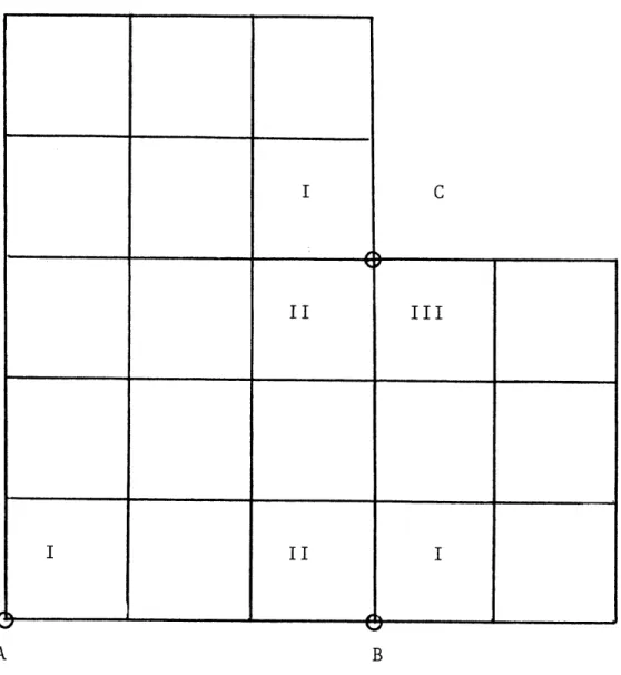
Generation of basis functions on the boundary can be considered as a special case of the above considerations. These are obtained by coupling element functions whose sup-ports are nonzero (i.e., element functions which are nonzero

in a particular boundary region). For example, consider the portion of a rectangular mesh as shown in Fig. 8. The basis

functions at point A coincide with element functions in region I. The basis functions at point B are obtained by coupling two element functions in regions I and II. Finally, the basis functions at point C are obtained by coupling three element functions defined on regions I, II, and III.

As in the one-dimensional case, it can be shown [7] that for the Hermite interpolate s(x,y) {given by Eq. (34)] of the function satisfying the weak form of the two-dimensional

of a Rectangular Mesh

A B

diffusion problem, the error bounds are 8(px~p )KA (2m -p X)+ apxa p y

(f(x,y)-s(x,y))|I

)

+--l<i<M -1 li+1i-il- A _l<j<N- max _{1 j+1~ j , a}and K

and K are constants independent of Ti and A. Consequently,

for the case of bilinear and bicubic Hermite interpolation we have the following interpolation error bounds:

2 2

If(x,y)-s(x,y)|| L <Kx 1Ax + K ₁ Ay (bilinear)

4 4

<Kx,₂Ax + Ky,₂Ay (bicubic).

K ,K and Kx, 2, Ky,2 are the upper bounds of K and K

for the bilinear and bicubic approximations, respectively.

3. Varying Cross Sections within the Expansion Element

We have tacitly assumed up to this point that the diffusion coefficient is a piecewise constant function. However, the weak form of the diffusion problem is properly posed for a more general behavior of the diffusion coef-ficient. In particular, a unique solution to the problem

will exist if D(x,y) takes the form of a piecewise con-tinuous function rather than a piecewise constant function.

From the theoretical viewpoint, piecewise continuous diffusion coefficients present no particular difficulties.

From the viewpoint of approximation methods, the change merely alters the evaluation of elements in the coefficient matrix.

The number of basis functions or unknowns is approxi-mately equal to some integer times the number of mesh points, and we assume that mesh points are always located at element

interfaces. If the system we are modeling has many material

discontinuities, then we will have many unknowns. It is

evident, therefore, that if the spacing between material discontinuities is very small, then finite difference meth-ods may be adequate for the problem, and one need not con-sider higher-order methods. On the other hand, it seems attractive to use coarse meshes with some higher-order

method in an attempt to arrive at accurate solutions with a

small computing burden. For highly heterogeneous systems,

it is clear that we must consider the problem of mesh ele-ments which extend over material discontinuities. Finite

elements techniques incorporated in the code CHD were devel-oped to address this problem.

The techniques employed in CHD use element and/or basis functions which are smooth within their region of definition. Material property discontinuities within this region are

accounted for in the basis function inner products. The

approximate solution, therefore, will be smoother than the actual solution, although the effects of the discontinuities

will be averaged into the approximate solution through the elements of the coefficient matrix.

4. Matrix Formulation of the Multigroup Diffusion Problem

We now present the matrix form of the equations which result from the application of the finite element method to

the multigroup diffusion problem.

As was done in the development of the two-dimensional basis functions, we will consider a partition of the problem

domain in Cartesian coordinates. The partition will place M mesh points along the x-axis and K mesh points along the

y-axis. As for physical considerations, a PWR analysis, for

instance, which uses a mesh grid coinciding with the core assembly interfaces produces remarkably accurate results.

Consider now Eq. (20a) specialized to the cases of

general downscattering (with no upscattering) and no extraneous

source (which defines an eigenvalue problem). The

within-group scattering cross section is subtracted from the total cross section to form the removal cross section, Z

rg Thus we have

-V-D1 VD $1 (x,y) -V-D V( (x,y) SErl ₁

_(xy)

group flux approximation

M N K(i,j) D (x,y) = Y X I g i=1 j=l k=l can be written as g a.. u..k(x,y),

where K(i,j) is the number of basis functions at point

It i assumed that M, N, and K(i,j) are the same for all energy

groups. We apply the Galerkin scheme to the weak formulation

of Eq. (41) and that 5 satisfies

+ (Erl 1,uijk)Q = G Xi = A fg'g, ijk Q gA-(D V _{Vu ijk)Q2+ rg (Dg, uijk)Q} g-l ug X g=2, sgg' g, ,u G. for i=l, j=l, k=l, where (u,v) ... , M ... , _{K(i,j) I} = f uvdV.

Rewritten in matrix operator form, Eq. (43) becomes

S- F} a -X G 9 g (x,'y) (x~y) fgI g The ,(x,y), (41) (42) (ij). G g = 1 ijk) Q' (43) (D 1 _{,llv uijk G} I v X, {& 0, 1 (44)

where

al, *.., ajG1

The form which the a takes can be seen from examination of

Eq. (42).

In a two-group problem, for example, Eq. (44) can be written in the general form

[0 _O

LJ( a

X

_F

ja

I " Is

=21 =221 -2 -21 O-2'

or, as two coupled matrix equations,

L a [El[Fa, + Fa]

-l -1 11: - =12-2J

L a , F a 2] a(46)

- 22 2 1 22 21 1

where the L matrices incorporate the diffusion and removal

=g

terms the Fg, matrices incorporate the fission terms, and

the S₂1 matrix incorporates the group 1 downscattering terms.

The term F2 1a, is the source of fission neutrons to group 2

arising from fissions occuring in group 1, and F2 2 22 is the

source of fission neutrons to group 2 arising from fissions occuring in group 2. In the usual two-group analysis,

however, these two particular fission sources are assumed to

be negligible (i.e., x2=0), and Eq. (46) reduce to the more

common form of the two-group equations,

L1 1 I [ a= +

(47) k2-2 = 21 11

A few comments should be made regarding the forms of