CHANGE IN RESIDENTIAL PRICES: A Cross-Sectional Time-Series Analysis
for the Boston Metropolitan Area by
ANNE E. KINSELLA B.A., Economics
Clark University, Worcester, MA (1985)
Submitted to the Department of Urban Studies and Planning in Partial Fulfillment of the Requirements of the Degree of
Master in City Planning and
Master of Science in Real Estate Development at the Massachusetts Institute of Technology
February 1991 Anne E. Kinsella
The author hereby grants to MIT permission to reproduce and to distribute copies of this thesis document in whole or in part.
Signature of Authort{ u
Afine E. Kinsella Department of Urban Studies and Planning January 18,1990
Certified by
-7i
i1( byLyna L. WigginsAssistant Professor, Depa ment of Urban Studies and Planning
Thesis Supervisor
3JT'nuary 18, 1990
Accepted by
Phi lip L. Clay Associate Professor, Director MCP Program Accepted by
Gloria Schuck Director of Education Interdepartmental Degree Program in Real Estate Development
CHANGE IN RESIDENTIAL PRICES: A Cross-Sectional Time-Series Analysis
for the Boston Metropolitan Area by
ANNE E. KINSELLA
Submitted to the Department of Urban Studies and Planning in Partial Fulfillment of the Requirements of the Degree of
Master in City Planning and
Master of Science in Real Estate Development at the Massachusetts Institute of Technology
February 1991
ABSTRACT
In this thesis a pooled time-series cross-sectional analysis of rates of appreciation in single family home prices was conducted at the intra-regional level. The window of analysis included 103 individual or combined cities and towns within the five counties comprising the Boston Metropolitan Area: Essex, Plymouth, Middlesex, Norfolk and Suffolk.
The raw database used embodied all real estate transactions, commercial as well as residential, which occurred within the study area between 1983 and 1989, the time-frame for this analysis. From this database appreciation rates in single family home prices were estimated employing a weighted repeat sales regression model. This model was run subsequent to a series of measures taken to improve data integrity, including: address correction; elimination of all transactions on other than single family homes; removal of outlying observations; and inflation adjustment.
After calculating rates of appreciation in single family home prices by community, by year, a number of fiscal, demographic and location specific variables were introduced to explain differential rates of appreciation across time and space. Finally, spatial analysis of the data and regression results was performed using thematic mapping tools to aid interpretation of the model.
The regression results demonstrate that during periods of economic vitality, as was evident in the study area during the mid 1980s, communities generally viewed as less desirable exhibited higher rates of appreciation in home values than other localities, due to the effects of market speculation. In contrast, during periods of stable growth or decline, home buyers tend to be more risk averse, thus more attractive communities with favorable packages of public goods and amenities fared better.
Thesis Supervisor: Lyna Wiggins
Title : Assistant Professor, Department of Urban Studies and Planning
CHANGE IN RESIDENTIAL PRICES: A CROSS-SECTIONAL TIME-SERIES ANALYSIS FOR THE BOSTON METROPOLITAN AREA
CHAPTER 1: INTRODUCTION: PROBLEM STATEMENT 10 CHAPTER 2: REVIEW OF RELEVANT LITERATURE 15 A. The Determinants of Housing Prices 15
1. Structural and Property Characteristics 16
2. Fiscal and Financial Determinants 17
a. National Level 17
- Mortgage Interest Rates 17
- Personal Income Tax Rates 17
b. Local Level 18
- Property Tax Rates 18
- Educational Expenditures 21
- Other Fiscal Variables 23
3. Locational Determinants 24 a. Zoning 24 b. Land Use 25 c. Density 25 d. Accessibility 26 e. Owner Occupancy 28 4. Population Characteristics 28 a. Income 28 b. Employment 30 c. Racial Composition 30 d. Poverty Rate 31 e. Crime Rate 31 f. Population 32 g. Age Composition 33
B. Measures of Housing Price Change 37
1. Median Sales Price 37
2. Hedonic Price Indices 38
3. Repeat Sales Method 40
C. Conclusions 41
THE CONTEXT: ECONOMIC CONDITIONS OF THE 1980 A. The National and Regional Picture 42
1. Income 43
2. Employment 45
3. Unemployment 49
4. Construction and Mortgage Lending 49
B. The Study Area 53
CHAPTER 4: METHODOLOGY 69
A. Dependent Variable: The Weighted Repeat Sales Model 70 1. Data Set Preparation:
Selection and Aggregation of Municipalities 74 2. Quantifying Real Housing Price Appreciation 75
a. Data Clean-up 78
b. Elimination of Erroneous and Extreme Cases 78
c. Inflation Adjustment 80
B. Variables Chosen to Elucidate Housing Price Differences 82 1. Financial and Fiscal Determinants 84
a. National Level 84
b. Local Level 84
- Effective Property Tax Rates 84
-Dummy Variable for Differential Tax Rates 87
-Educational Quality 88 2. Locational Factors 90 a. Percent Residential 90 b. Percent Industrial 91 c. Density 91 d. Residential Construction 92 e. Accessibility 94 - Automobile 96 - Public Transit 98 3. Population Characteristics 99
a. Department of Revenue - CACI Adjustment Methodology 99 b. Real Median Household Income 101
c. Unemployment Rate 102 d. Racial Composition 103 e. Number of Households 103 f. Age Cohorts 104 Page 5 CHAPTER 3:
MODEL RESULTS
A: Housing Price Appreciation Index: WRS Regression Results 108
B: Model Specification 109
1. Overall Model Fit 109
2. Fiscal Determinants 119
a. Effective Property tax Rates 122
b. Dummy Variable for Differential Tax Rates 129
c. Education 131 3. Locational Factors 136 a. Percent Residential 136 b. Percent Industrial 137 c. Density 139 d. Housing Permits 143 e. Accessibility 146 4. Population Characteristics 149 a. Income 151 b. Unemployment 155 c. Percentage White 156 d. Number of Households 157 e. Age Cohorts C. Conclusions 163
CHAPTER 6: CONCLUDING REMARKS 164
A. Usefulness of the Model 164
B. Improvements to the Existing Data 166
C. Improvements to the Model Specified 167
D. Additional Variables of Interest 170
a. Fiscal Factors 170
b. Locational Amenities 171
c. Demographic Factors 172
E. Other Model Specifications 173
F. Concluding Remarks 174
Page 6
108
Appendix A: Weighted Repeat Sales Model
Appendix B: Observations Lost through Data Clean-Up Appendix C: Massachusetts Property Tax Law
Appendix D: Central Transportation Planning Study:
Methodology Employed for Development of the Time and Distance Matrix.
Appendix El: CACI Update Methodology
Appendix E2: Explanatory Variable Calculations
Appendix F: Correlation Matrix
SOURCES CONSULTED 176 177 178 Boston Area 179 184 192 201 202 Page 7
LIST OF TABLES AND FIGURES:
Age at Marriage, By Sex Divorce Rate, By Sex
Wage and Salary Income Growth: Average Annual Percent 44 Nonagricultural Employment: Average Annual Growth 46
Nonmanufacturing Employment by Industry: Average Annual Growth 48
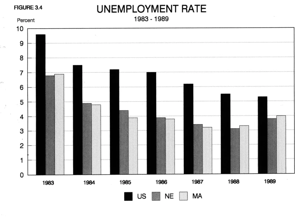
Unemployment Rate 50
Selected Assets of Commercial Banks 52
Housing Permits Authorized, Indexed to 1983 54
Median Sales Price: Existing Single Family Homes 55
Total Population and Town Counts Per County 56
Map of Counties in the Boston Metropolitan Area 57
Map of Essex County Cities and Towns 58
Map of Middlesex County Cities and Towns 59
Map of Norfolk County Cities and Towns 60
Map of Plymouth County Cities and Towns 61
Map of Suffolk County Cities and Towns 62
Countywide Housing Price Appreciation Rates, 1983 and 1984 64 Countywide Housing Price Appreciation Rates, 1985 and 1986 65 Countywide Housing Price Appreciation Rates, 1987 - 1989 66
Single Family Home Transactions, by County 71
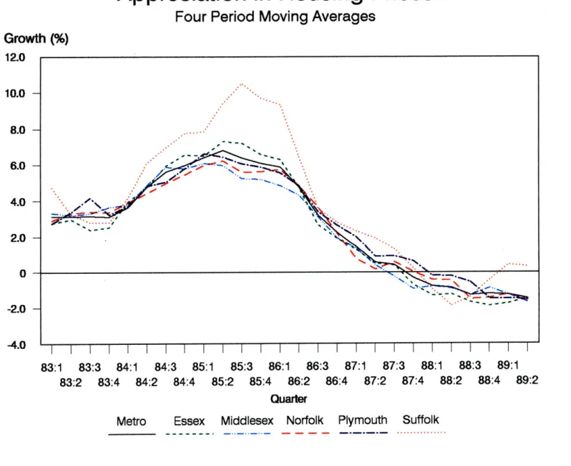
Countywide Quarterly Appreciation in Housing Prices: Four Period Moving Average, 83:1 - 89:2 73
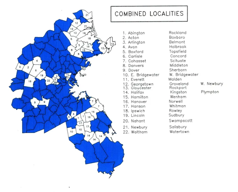
Combined Localities 76
Eliminated Localities 77
Consumer Price Index 81
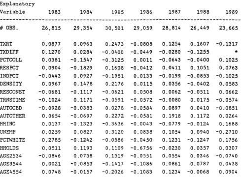
Explanatory Variables Analyzed 83
Localities with Differential Tax Rates 86
Employment Centers Outside of the Boston CBD 97
Model Formulation 106 Page 8 Chapter 2 Table 2.1 Table 2.2 Chapter 3 Figure Figure Figure Figure Figure Figure Figure Table Figure Figure Figure Figure Figure Figure Figure Figure Figure 3.1
3.2
(
3.3
(
3.4 3.5 3.6 3.7 3.1 3.8 3.9 3.9 3.9 3.9 3.9 3.10 3.10 3.10 a,b) a,b) a b C d e a b c Chapter 4 Table 4.1 Figure 4.1 Figure Figure Figure Table Table Figure Table 4.2 4.3 4.4 4.2 4.3 4.5 4.4Chapter 5 Table 5.1 a Table 5.1 b Table Table 5.2 5.2 Table 5.2 c Table 5.3 a Table 5.3 b Table 5.3 c Figure 5.1 Figure 5.2 Figure Figure Figure Figure Figure Figure Figure Figure Figure Figure 5.3 5.4 5.5 5.6 5.7 5.8 5.9 5.10 5.10 5.10
Correlation Matrix, Dependent Variable
with all Type-Specific Variables 111
Correlation Matrix, Dependent Variable
with all Time-Period Variables 111
Full Model and Type-Specific Regression Results: All Variables 112 Full Model and Type-Specific Regression Results: 113
Excluding Property Tax Rates
Full Model and Type-Specific Regression Results: 114 Excluding Multicollinear Variables
Time-Period Regression Results: All Variables 115
Time-Period Regression Results: Excluding Property Tax Rates 116 Time-Period Regression Results: Excluding Multicollinear Variables 117
Real Annual Rate of Appreciation in Single Family Homes:
By Municipality 119
Indexed Assessed Property Value as a Percent of Indexed
Rates of Housing Price Appreciation 127
Effective Property Tax Rate 128
Municipalities Utilizing Differential Property Tax Rates 132
Percent of High-School Graduates Attending Four Year Colleges 135
Density - 1985 Levels 142
Lagged Value of Residential Permits Per Existing Residential Parcel 145
Median Household Income 151
Unemployment Rate 154
Percentage of the Population Between 25 and 34 Years Old 160 Percentage of the Population Between 35 and 44 Years Old 161 Percentage of the Population Between 45 and 54 Years Old 162
CHAPTER 1
INTRODUCTION: PROBLEM STATEMENT
During the 1980s housing prices in Boston and many other metropolitan areas across the country experienced a period of unprecedented appreciation, followed by an abrupt decline. In the Boston area, appreciation, caused largely by market speculation, sharply influenced the affordability of homes, prohibiting individuals and families from attaining the 'Great American Dream' of homeownership. As property values continued on their upward course, developers, recognizing an opportunity for profit joined on the bandwagon, and residential development of both single-family homes and condominium units increased dramatically.
By the end of the decade, a surplus in the housing stock was apparent, and numerous
property foreclosures resulted in the insolvency of many financial institutions. As a result of this sharp turn in the real estate market Boston became characterized as 'the Houston of the 1990s' during the last decade of the twentieth century. Most of the studies conducted during the late 1980s and early 1990s focused on both the cause of this market bubble, and its inevitable burst. Few, however, have endeavored to ascertain the impact of traditional housing price determinants such as accessibility, density, property tax rates and income, too name just a handful, during periods of nontraditional market
expansion and contraction. This final issue will be the focus of this thesis.
Historically, studies have attempted to identify the determinants of changes in housing demand and/or its price component (D = P *
Q).
Most of these studies have been limited to analysis either across location or time. Locational studies examine differences across regions of the country, or among communities within a region or metropolitan area. Time-series studies focus on changes induced by national or regional economic cycles, long-term trends, seasonal and irregular fluctuations. Studies endeavoring to describe and explain variations in housing prices across the dimensions of both time and space have been sparse.For this thesis I conducted a pooled time-series cross-sectional analysis of appreciation in single-family home prices at the municipal level. The window of analysis included cities and towns located within the Boston Metropolitan area, and the time frame was the period from 1983 through 1989. My focus here was on how intra-jurisdictional
differences in public goods and amenities affected rates of single family housing price appreciation during this period. As mentioned above, the boom period of the 1980s was of particular interest because it provided an arena for testing whether the traditionally assumed effects of financial and fiscal variables and amenities remain stable during periods of robust economic expansion.
The results of this analysis do not support the theory of tax capitalization during periods
of exceptional market activity. In contrast, the findings of this study imply that in periods of flourishing real estate market conditions, those properties located in communities traditionally viewed as less desirable, may be considered undervalued. Thus rates of appreciation in the value of properties in less attractive municipalities tend to outpace appreciation rates on properties in communities commonly viewed as attractive.
I utilize community level measures of public goods and amenities as determinants community quality. For the purposes of this study, I classify these public goods and amenities into four major groups: structural characteristics, financial and fiscal determinants, locational considerations, and population characteristics. Structural characteristics of a property include factors such as building and lot size, number of bedrooms and baths, age of the structure, etc. Financial and fiscal determinants encompass variables such as mortgage interest rates, income and property tax rates, educational expenditures, expenditures on police and other municipal services, and debt service. Locational considerations embrace categories of zoning and land use, as well as density and accessibility. Population characteristics embody elements such as income, population, employment, racial composition, poverty population, and crime rates.
In Chapter Two I evaluate the existing literature, addressing the significance of various determinants of housing price disparities. The premier work on financial and fiscal factors was Charles Tiebout's (1956) theory which stated that locally produced public
goods and property taxes will affect housing prices. I begin with the Tiebout
presumption, and consider modifications of his theory introduced by other academics and scholars. In addition to evaluating variables of possible interest for inclusion in this model, I review alternative techniques for measuring the dependent variable (variations in rates of housing price appreciation across localities) expounding on the benefits and faults of these techniques.
In Chapter Three I discuss variations in the national, New England, and Massachusetts economy during the 1980s. Following a mild recession early in the decade, the New England region and Boston Metropolitan Area experienced a period of unprecedented expansion. The regional growth greatly exceeded the growth occurring nationally. As the decade drew to a close, however, regional growth stagnated and began to decline while national expansion continued, although at a modest pace. The unique context of the Boston Metropolitan area during the 1980s make it an ideal case for analysis of changes in housing prices.
In Chapter Four I select the most appropriate method for analyzing rates of appreciation in housing prices, and model differential rates across locations, utilizing fiscal, demographic, and locational variables. Descriptions of the variables included in the final model, and the methodology for compiling annualized measures of these variables by locality, are included in Chapter Four.
The model results are presented and discussed in Chapter Five. In this analysis I ran a series of models in order to ascertain both the spatial and time period effects on rates of housing price appreciation. These sub-models focused on the differential impacts of the various determinants of appreciation in urban, suburban, and exurban areas, during periods of economic expansion and decline. I employ the thematic mapping capabilities of Geographic Information Systems (GIS) technology in this chapter as a tool for analysis. These thematic maps more clearly depict locational and time-series variations, thus simplifying this complex analytical task.
In Chapter Six I present my conclusions. In addition, I address potential improvements to the model specified, and pose questions that would be of interest in future research. Given the abundance of data compiled for this study, a wealth of alternative analytical questions could be considered, and more valuable insight into the peculiarities of the Boston real estate market during the 1980s, commercial as well as residential, revealed.
CHAPTER 2
REVIEW OF RELEVANT LITERATURE
In this chapter I review the relevant literature which examines the effects of local disparities in the availability of public goods and amenities on housing prices. In the first section of the chapter, I focus my attention on the variables most frequently cited in interpretive studies of housing prices. I follow this discussion with a review of
alternative methodologies for gauging changes in housing prices. Past housing studies have been conducted at various levels of aggregation: national, inter-regional (comparisons across Metropolitan Statistical Areas (MSA)), and intra-regional (comparisons among cities and towns within a state or MSA). Methodologies chosen have also varied from modeling techniques (OLS, Two-Stage LS, GLS, etc.) to surveys attempting to discern which factors most significantly influence a home buyer's decision to purchase a particular property. This review encompasses both inter- and intra-regional studies, and examines models utilizing a variety of these techniques.
THE DETERMINANTS OF HOUSING PRICES
Four categories of variables have most frequently been identified as explanatory variables in housing price regression models. Measurements of structural and property characteristics, most often utilized in hedonic price models (total square footage of a
home, number of rooms, lot size); financial and fiscal determinants, at the national level (mortgage interest rates and federal income taxes), and at the local level (property tax rates, educational expenditures, and other municipal expenditures); locational factors (density, measures of distance or access to a major employment node, housing starts, crime rates); and population characteristics (population, median family or household income or wealth measures, (un)employment, age, educational levels, race, poverty population). These four categories of explanatory variables are described in more detail in the following sections.
Structural and Property Characteristics
Structural characteristics greatly influence the price of a home. Other things being equal, a 2000 square foot home will command a higher price than a 1000 square foot home. Similarly, a home with a large lot or swimming pool will command a higher price than a home on a smaller lot or without a pool, ceteris paribus. Hedonic price models have traditionally been used to control for variation in structural characteristics. A detailed discussion of hedonic models will be presented in the second section of this chapter.
Financial and Fiscal Determinants National Level
Mortgage Interest Rates
National level variables have greatly influenced the demand for housing by altering the price component of the demand equation. Mortgage interest rates have historically had a negative impact on housing demand, and thus price (Kau and Sirmans 1984, Case
1986, Case and Shiller 1990). During the 1980s, the introduction and increased utilization of variable rate mortgages altered the certainty of housing expenditures and changed the effect of mortgage interest rates on the housing market. With fixed rate mortgages, an individual would purchase a home, acquire financing, and be guaranteed that a fixed payment would be required to pay off the mortgage. Variable rate mortgages caused fluctuations in mortgage payments, but allowed households to choose between risk, as variable rate mortgages run the risk of higher future mortgage payments due to changing interest rates, and return, as the base interest rate on fixed rate mortgages exceeds that of variable rate mortgages.
Personal Income Tax Rates
Personal income tax rates have also had a substantial effect on housing prices as changes in the deductibility of homeowner related expenses (mortgage interest, insurance, etc.) have resulted in changes in the true value or cost of property ownership and, consequently, an individual's wealth (Case and Shiller 1990). Grebler and Mittelbach
(1979) conducted a survey of home buyers motivations for purchasing homes in 1975 and
1977 in Contra Costa and Orange County California, and found that approximately
two-thirds of those investing considered income tax benefits of home ownership important in their decision. Furthermore, this tax benefit or subsidy increases with income, as marginal income tax rates have different effects on different income levels.
Local Level
Property Tax Rates
The pioneering work in the theory of the value of local expenditures and amenities to consumers of housing services was introduced in 1956 by Charles M. Tiebout. Tiebout utilized an assortment of local municipal finance variables -including property tax rates, educational expenditures, police and fire protection, and amenities (e.g., a public beach or golf course) -and determined that such variables strongly influence intra-metropolitan movements of the population. The Tiebout model had households choosing between urban and suburban localities based on the distribution of fiscal expenditures within a locality and not simply on variations in the income elasticity of demand for land. Tiebout stated "The consumer-voter may be viewed as picking the community which best satisfies his preference patterns for public goods (Tiebout 1956, 418)."
Tiebout's theory was based on a number of assumptions, some of which he and/or others recognized as weak. These assumptions were:
1. Consumers are fully mobile and base their locational choice on the fiscal
characteristics of a community, choosing that locality which best fulfills their preferences.
2. Consumers are assumed to be fully aware of variations in fiscal expenditures across communities.
3. The pool of communities available from which the consumers may choose
is large.
4. Employment opportunities are assumed to be identical among localities.
5. Public services supplied exhibit no economies or dis-economies of scale.
6. The optimal size of a community can be determined because a community
has fixed resources, and is defined as the size at which average cost of the bundle of fiscal services provided is minimized.
7. Localities which fall below this optimum will seek to attract new residents
while those above the minimum will attempt to deter them.
Since the publication of Tiebout's theory, numerous articles have been written critiquing his assumptions. In many of these articles, additional variables have been introduced to explain locational choice and/or resulting changes in housing values across locations. None of these studies have rejected the importance of property tax rates in determining location. However, Oates (1973) concluded that shopping among communities was more
evident in suburban locations relative to the city. In his intra-regional analysis of 53 northern New Jersey commuting suburbs of Manhattan, Oates found that people were willing to pay relatively more for higher quality services or would choose locations with lower taxes where services of identical quality were offered. Wilson (1979) reiterated these findings. In his inter-regional analysis, Wilson concluded that higher quality residential packages relative to low tax rates were found in the suburbs, when compared with cities.
Hamilton (1975) expanded on Oates' conclusion and determined there exists a differential effect of property taxes in cities and suburbs; in the cities property taxes are viewed as an excise tax on housing while in the suburbs property taxes are regarded as a payment for services. Ihlanfeldt (1984) concurred with Hamilton in his estimation of housing demand equations for 30 SMSA's. Ihlanfeldt found that, if anything, higher tax payment is associated with a greater purchase of housing services in the suburbs, while in the city these payments do indeed act as an excise tax. Mills and Oates concluded that, "most central cities are almost certainly too large and too diverse to be able to provide public service bundles tailored to the needs of particular segments of their populations, and constitutional considerations greatly limit their ability to do so (Mills and Oates 1975,
9)."
All of the studies reviewed concluded that property tax rates bear a negative relationship
to housing prices, thus supporting the theory of tax capitalization. This theory states that
increased tax rates will result in lower property values, ceteris paribus. Studies of tax rate measures have been conducted in numerous ways. Levin (1982) postulated, given that market forces work, home prices in areas with higher effective tax burdens will grow more slowly than in areas where the effective tax burden is lower, other things equal.
Oates (1969), Levin (1982), Ihlanfeldt (1984) and Michaels and Smith (1990) advocated use of the effective or full value property tax rate to correct for differential assessment ratios among communities. For example, assume the characteristics and expenditures of Town A and Town B are identical. The property tax rate in Town A is 20 mils ($20 per
$1000). Town B has a property tax rate of 15 mils. Thus, the rational consumer of
housing services would choose to locate in Town B in order to minimize his or her property taxes. However, if this discrepancy in property tax rates is due to an assessment rate of 75% in Town A (.75 * 20 = 15) versus 100% in Town B (1 * 15 =
15) the consumer will be indifferent to the two locations, as the actual tax levy will be
identical.
Educational Expenditures
In studies that have evaluated property tax rates and municipal expenditures, the primary category of expenditures included has been education. Oates (1969) advocated use of per pupil educational expenditures because this variable is the largest single cost item in most municipal budgets. He used the natural logarithm of educational expenditures per pupil
as a proxy for educational quality in his analysis of New Jersey communities. Hamilton, Mills and Puryear (1975) concurred with Oates, and utilized educational expenditures as a surrogate for public services because it accounted for more than half of local government expenditures and had an income elasticity of demand substantially greater
than zero.
Other studies where per pupil educational expenditures were utilized as a proxy for educational quality, and where a positive relationship was postulated between this variable and housing prices, include Tiebout (1956) and Hamilton (1975). Izraeli (1987) conducted a similar analysis at the inter-regional level, examining determinants of housing value and monthly rents in over two-hundred SMSA's in the U.S. He found per pupil educational expenditures to be a statistically significant predictor of housing values
at the .05 % level.
Alternative measures of educational quality have been recommended by others. Rosen and Fullerton (1977) re-estimated the Oates model at the inter-regional level. Using a four year panel study which followed movers, they replaced Oates's per pupil educational expenditure variable with grade-level performance of fourth graders on standardized tests of reading and math and found a positive and significant relationship between test scores and housing values. Michaels and Smith (1990) examined pupil-teacher ratios in suburban Boston school districts and found a negative relationship between this variable and property values; this translates into a positive relationship between school
expenditures and property values as more teachers translate into higher costs.
Other Fiscal Variables
In addition to educational quality measures, many studies have evaluated the relationship of housing values to other municipal expenditures including police, fire, debt service, and other variables. In response to criticism by Pollakowski (1973), Oates (1973) redefined his earlier model by including a variable for all non-school related municipal expenditures in his intra-regional analysis of New Jersey communities, and found a positive relationship with property values, as would be expected under the Tiebout hypothesis. Although Oates acknowledged the significant predictive value of these non-educational municipal expenditures, he maintained that if tax capitalization does occur, it appears to be more strongly associated with educational expenditures than these other public services. Izraeli (1987) also discerned a positive relationship between housing
values and non-educational expenditures across SMSA's.
Kohlepp and Ingene (1979) conducted an intra-regional analysis of thirty-nine suburban Columbus, Ohio communities. In this analysis they separated local public services into five categories, one of which was per pupil expenditures, and found that only this category exhibited a positive significant relationship with property values. In general, police and fire expenditures have exhibited a positive relationship with housing prices while debt service has maintained a negative relationship. Educational expenditures, however, have consistently asserted a far greater impact on home prices than these other
municipal expenditure categories.
Locational Determinants Zoning
In addition to Hamilton's criticism of the differential effects of property taxes on urban versus suburban locations, he further criticized Tiebout, stating that, "(the) Tiebout hypothesis seems to be a formula for 'musical suburbs' with the poor following the rich in a never-ending quest for a tax base (Hamilton 1975, 15)." Hamilton argued that exclusionary zoning, in the form of minimum lot size requirements, acts as a pricing mechanism: "...in an urban area with a large number of independent jurisdictions, judicious use of zoning can convert the residential property tax into an efficient price for
local public services (Hamilton 1975, 13)." Tiebout (1956) would not dispute this criticism, and in his article on the theory of local expenditures he acknowledged that communities may utilize restrictive zoning laws to maintain or attain optimum size. However, he contradicted this statement with his first and third assumptions of full mobility and a large number of communities from which to choose. By imposing zoning restrictions, individuals are limited in their available choice of locations unless they possess the financial means to overcome these limitations. Mills and Oates (1975) also concluded that communities rely on land use regulations by which residents can regulate, to a certain extent, entry into the community.
Land Use
Non-residential property uses have generally had a negative impact on residential property values. As White (1975, 37) states, "...without some inducement communities would prefer to exclude business and factories from their borders." This effect is much more pronounced when the non-residential use is primarily industrial as opposed to commercial. Noise (Mieszkowski and Saper 1978) and pollution (Anderson and Crocker
1971, Izraeli 1987) have been determined to negatively impact property values and these
disamenities are more prevalent among industrial properties.
Density
Michaels and Smith (1990) examined average lot size as a substitute measure of zoning in their survey of housing prices in suburban Boston communities, and determined a positive and significant (at 1 %) relationship existed between average lot size and housing prices. Population per area or density is another proxy measure for zoning. However, density may also exhibit a strong negative relationship with accessibility to major employment nodes. Exclusionary zoning in a community will result in larger lots and correspondingly lower density as more land is required per housing unit.
Lower density and open space have been shown to exhibit positive impacts on housing prices as open space is a highly valued amenity, particularly in densely populated regions of the country. Correl, Lillydahl and Singell (1978) studied the effects of greenbelts on residential property values in the city of Boulder, Colorado. This city was chosen as the
subject of analysis because in 1967 residents of Boulder approved a proposal to establish a fund for purchasing and managing greenbelts. This fund was to be financed by a 0.4 percent city sales tax. As of 1978 the Boulder Open Space Program had purchased some
8000 acres. Correl, et al. determined that distance from a greenbelt had a statistically
significant negative impact on the price of residential property. Thus the greenbelts acted as a quasi-public good, disproportionately benefitting resident living in close proximity to this open space.
Accessibility
It is well established that residential choice of location is influenced by proximity to workplace. Therefore, accessibility should significantly affect housing prices. In a number of intra-regional studies, access measures have been confined to distance to the Central Business District (CBD), and the relationship to housing prices has consistently been negative.
Oates (1969) used linear distance to examine accessibility to Manhattan in his cross-sectional analysis of New Jersey commuting suburbs. He assumed, "within a metropolitan area the accessibility of the community to the central city should be of importance. Therefore, ceteris paribus, we would expect property values to vary inversely with distance to the central city (Oates 1969, 959)." Wingo's (1961) theory also assumed all employment was fixed in the CBD. In Wingo's model, a household was assumed to choose a location which minimized the sum of transportation costs to the
CBD and land use costs associated with the amount of land being consumed. Alonso (1964) likewise had households choosing location and land consumption as a tradeoff between cheaper rents and longer trips to work in the CBD. Jud (1985) included a variable measuring accessibility to downtown San Francisco and Los Angeles in his examination of the effects on home values in communities in these areas, and found the relationship to be negative and significant.
The main criticism of housing price models including only access to the CBD is that most urban areas have multiple employment nodes. In addition, technological advances in the area of computers and fiber-optic networks during the 1980s resulted in expansion of the market for back offices, thus increasing demand for office space outside the CBD. In the early 1990s these trends continued to support the development of multiple employment centers as leasing costs in suburban locations were more economical than in the CBD.
Strazheim (1975) criticized the models which assumed one central workplace as an apparent attempt to minimize analytical complexity. Successive models have attempted to prototype multiple employment nodes. Michaels and Smith (1990) used a weighted distance measure to various employment centers in the Boston MSA and discerned a significant (at 1 %) negative relationship between distance and home prices. Johnson
(1982) delved more deeply into the accessibility variable by including in his hedonic
price model the natural logarithm of the sum of distances to employment centers, where
distance was weighted by the proportion of total employment in that center.
Owner Occupancy
Dwelling types vary significantly across location and have been determined to affect housing values. Oates (1969) used median household income as a proxy for desirability of a neighborhood but recognized a problem in using this variable because he was actually interested in modeling only homeowners' income. In communities with a large number of renters, using median income to approximate the income of owner occupied dwellings tends to underestimate its true value, as proportionally more of the lower income residents of a community tend to be renters.
Other studies have included a measure of owner-occupancy to help explain housing values. In their suburban Chicago study, Anas and Eum (1984, 1986) examined the proportion of single family dwellings in the area, and found a positive (at 5%) relationship between this variable and home prices.
Population Characteristics Income
Aside from property taxes, income is the determinant most frequently included in housing price models. Reid (1962) evaluated this relationship at the intra-regional level. Based on a group of households within a metropolitan area, stratified by census tract and housing quality, Reid found income elasticity of housing to be as high as two for
homeowners.
A number of measures of income have been used in previous work including disposable
income, per capita income and average family income. deLeeuw (1963) utilized disposable personal income in his analysis, and found this variable to be a significant positive determinant of home-buying units. Strazheim (1975) modeled intra-metropolitan variation among housing submarkets and determined average income to be a positive significant predictor of housing demand. Anas and Eum (1984) evaluated the effects of average family income on housing prices in suburban Chicago and also detected a positive significant (at 5 %) relationship.
Other analysts perceived this positive relationship by employing measures of median income, arguing that average income values in a community or metropolitan area may be skewed upward by the presence of a few wealthy inhabitants. As mentioned previously, Oates (1969) included median family income as a proxy for intangible characteristics (e.g., beauty, neighborhood attractiveness) of New Jersey suburban communities, and ascertained that this variable exhibited a positive and significant (at
1 %) relationship with home values. Jud (1985) employed median household income in his analysis of home prices in San Francisco and Los Angeles communities. This measure is more appropriate than family income measures because a single household may consist of multiple families. The most appropriate measure in the analysis of home purchase prices, as indicated by Oates (1969), is median homeowners' income. Izraeli
(1987) utilized median income of homeowners as a measure across SMSA's and found
a positive significant (5 %) relationship.
Employment
Case (1986) found the price elasticity of homes with respect to employment to be .82. In his model of a sample of Boston municipalities, Case estimated the log of total housing starts in double log form and solved simultaneously for price in order to evaluate the price-employment relationship. Case and Shiller (1988) surveyed housing consumers' opinions of the local economy, of which employment is a major factor, and found 29.5 percent of those surveyed in Boston, and 18.4 percent of those surveyed in Milwaukee, related the downturn in their respective local real estate markets to local economic conditions. In contrast, in the Anaheim, California, boom market, 25.4 percent of those
surveyed attributed the upturn to improvements in the local economy.
Racial Composition
Racial composition of a community has also been determined to relate to differential rates of appreciation in home prices. Kain and Quigley (1975) examined the St. Louis housing market and determined that race was positively related to housing price levels. Because of discrimination, blacks faced limited housing choices and as the black population increased during the 1950s and 1960s, prices in communities of color were actually driven higher than prices for identical homes in primarily white communities. In contrast, Anas and Eum (1984, 1986) concluded that a significant (at 5%) negative
relationship existed between property values and the proportion of blacks in Chicago suburban communities. Ihlanfeldt and Vazquez (1986) used data from the Annual Housing Survey of the Atlanta SMSA for the period April 1978 to March of 1979 and found race to exhibit a negative and significant relationship with home values at the .01 level. In this study a negative relationship was also expected as the market effects observed by Kain and Quigley were not as prevalent in the 1980s as they had been a quarter century earlier.
Poverty Rate
Rates of poverty vary across location, and higher rates of poverty have been demonstrated to relate to declining property values (Izraeli 1987, Oates 1963).
Communities with a substantial poor population tend to be characterized by a large proportion of renters, as these impoverished residents are less likely to have the financial means to become homeowners. Furthermore, housing conditions in poorer neighborhoods are inclined to be worse than in more affluent areas. This may be caused
by a combination of the inability of residents to finance improvements, poor maintenance
of rental property by absentee landlords, and the presence of tax delinquent and vacant property.
Crime Rate
Housing consumers also highly value security, particularly those with children (Wilson
1979). Areas where crime is prevalent are considered undesirable places to live and
raise a family. Often, poorer neighborhoods, and wealthier neighborhoods in close proximity to these less affluent areas, tend to be victimized by higher crime rates than other communities. These factors and other negative demographic impacts associated with less affluent communities have historically had a negative impact on growth in housing values.
Population
Measures of change in the population have also been utilized in an attempt to explain rising home prices. Generally, an increase in population will cause an increase in consumer demand for housing services, ceteris paribus. If consumer demand can be
satisfied by additions to the supply of housing then prices will not tend to rise. Zoning laws, however, may restrict additions to supply, and housing prices may thus be bid up.
Izraeli (1987) examined population growth rates across SMSA's and did not find a significant relationship to changes in housing prices. Case (1986) found similar results in his study of five suburban Boston communities, as the population growth between
1976 and 1985 in Massachusetts (1 %) lagged behind the nation (10% +) while growth
in housing prices in the state exceeded national rates of appreciation. Others have argued that population growth is not an appropriate measure, especially during the 1970s and 1980s when this nation endured vast changes in traditional demographic trends. Russell
(1982) notes that postponement of marriage and other demographic trends peculiar to the
baby boom generation led to a rise in household formation. Thus a more appropriate
measure would be growth in households rather than population growth. Mankiw and Weil (1989) determine that there was a negative correlation (-.57) between growth in the total population and housing demand. They then chose to limit population growth to those over the age of twenty-one and detected a much higher correlation with housing demand
(.86). This data supports the household growth theory as most households are formed by adults over twenty-one years of age.
Age Composition
A number of studies, conducted primarily during the 1970s and 1980s have examined
variations in the age structure of the population and its effects on the housing market. Wilson (1979, 5) divides the family life-cycle into seven stages, each distinguished by
specific needs and either changing or constant family size. These seven stages are:
1. Marriage or household formation
2. Pre-child (constant size)
3. Child bearing (increasing size)
4. Child rearing (constant size)
5. Child launching (decreasing size)
6. Post child (constant size)
7. Widowhood, or family dissolution.
Wilson characterized the demands of households at each of these stages. In the first two stages access is of primary importance, both to consumer goods and place of work. The middle three stages are delineated by increased demand for homeownership of detached dwelling units. In addition, particularly during stages three and four, privacy, open space and the package of available residential services discussed above gain importance, (ie, school quality, open space, safe streets, accessibility to services).
The aging baby boom changed conventional patterns of the duration of each of these stages, and the age at which family heads entered each of these stages. Various definitions of the baby boom have been offered, but here I refer to the baby boom as the period between 1946 and 1964, with the peak in 1957, utilizing the definition offered by Mankiw and Weil (1989).
Traditionally, individuals who fall into the 18-25 year-old group, have remained at home with parents until marriage. Changing trends of the 1970s and 1980s resulted in an increase in heads of household living alone or with non-relatives, predominately in the 18-34 year-old age cohort. This group is referred to by the Census Bureau as "primary individuals". The rise in this group was a driving force behind the change in household incidence. In 1950, only 4 percent of the population between the ages of 25 and 34 were considered primary individuals, by 1980 this group comprised over 20 percent of all households (Russell 1982). Two additional trends caused an increase in non-family households: a delay in the age at which young adults married (Table 2.1); and a growth in the divorce rate (Table 2.2), particularly in the 30-45 year-old age cohort where the divorce rate is highest (Gruen, Gruen, and Smith 1982).
Table 2.1
Median Age at First Marriage
1960 - 1985
Year Male Female 1960 22.8 20.3 1965 22.8 20.6 1970 23.2 20.8 1975 23.5 21.1 1980 24.7 22.0 1985 25.5 23.3
Source: U.S. Census Bureau, CPR: Population Characterii
Table 2.2
Percentage of the Population Divorced
by Sex, 1960 - 1985
Year Male Female 1960 2.0 2.9 1965 2.5 3.3 1970 2.5 3.9 1975 3.7 5.3 1980 5.2 7.1 1985 6.5 8.7 stics, P -20.
Other trends peculiar to the baby-boom have been determined to effect the housing market. Along with delaying marriage, as mentioned above, baby boomers postponed child bearing once married, and families were smaller than previously. In addition, an increasing proportion of women entered the labor force, and locational considerations may have been altered in families where both heads of household worked.
Due to the changes evident during the 1970's and 1980's, particularly the increase in non-family households, a more appropriate representation of demographic trends would separate the first stage of Wilson's model of family life cycle into two groups, thus creating an eight stage cycle with stage one as household formation and stage two as marriage. Furthermore, I would argue that a more fitting characterization would be household life cycle rather than family life cycle.
Most researchers who have considered the baby boom generation and changes in household and family formation have recognized that these demographic variables have had a substantial impact on the housing market. There was disagreement, however, as to which effects have been most prevalent among which age groups, and what the effects will be during the 1990's. Russell (1982) argued that expansion of the 35-44 year-old age group, along with their unique demographic trends toward household formation mentioned above, led to an increase in housing demand. Rosen and Smith (1986) also found that the population in the 35-44 year-old age cohort had a positive and significant influence both on the demand for resale housing and its price.
In their study of the effects of demographic changes on the housing market Gruen, Gruen and Smith (1982) determined that the 25-34 year-old age group, who embody the bulk of first time home buyers, would be forced to purchase starter homes or condominiums in the 1980's, if they could afford any home at all. They also argued that the 35-44 and
45-54 year-old age cohorts comprised the trade up market in that decade, and these
households would use equity built-up to purchase traditional suburban single-family detached homes. In retrospect, these forecasts have proved valid.
Mankiw and Weil (1989) considered those between 20 and 30 years of age as those forming households, and predicted negative real growth to occur in housing prices between 1990 and 2010. Case and Shiller (1987), examined the consumption of housing units among 25-44 year-olds and found changes in this age group to be positive and
significantly related to changes in home prices. Ihlanfeldt (1986) scrutinized housing consumption patterns among age groups 26-40, 41-55 and 56+ in his study of 30 SMSA's, and found the coefficients to be collectively significant when evaluated with other explanatory variables but not individually significant. Ihlanfeldt (1986) also found that in his white suburban resident equation, the coefficient of the 26-40 year-old age
group was the highest, while the 41-55 age group had the lowest coefficient.
MEASURES OF HOUSING PRICE CHANGE
The variables mentioned above have frequently been utilized to explain variations in housing prices. In the following section of this chapter I evaluate alternative methodologies that have been utilized to quantify rates of appreciation in housing prices. In this section I discuss housing studies, most of which have endeavored to gauge housing demand, or its price component. Demand, however, is not an appropriate measure, as the quantity of housing demanded by consumers of housing services varies, and price is strongly influenced by this quantity. Models measuring the willingness to pay for housing services, or the price of these services are preferable, as long as they control for the level or quantity of housing services demanded by a home buying unit.
Median Sales Price
The National Association of Realtors (NAR) publishes monthly reports of home sales and provides quarterly reports of the median sales price of single-family homes in 54 metropolitan areas. The timeliness and availability of this data is advantageous, and thus
many housing studies have relied on median sales price of existing single family homes and/or new construction as their dependent variable (Oates 1969, Hyman and Pasour
1973, Izraeli 1987). The problem inherent in using median sales price to explain housing values across time and location is variations in the quality of homes. If homes were homogeneous, median sales price would be an appropriate measure of value. However, because homes differ both within a community and among communities, at a fixed point in time, and the quality of properties sold varies over time, utilization of
median sales price may result in a biased price index over time and space.
Hendershott and Thibodeau (1990) examined the relationship between median and constant quality house prices. They concluded that during the 1976 to 1986 period the NAR median house price figure overstated the increase in constant quality house prices
by about 2 percent per year. The NAR acknowledges the potential bias in their data and
offers these words of warning and advice in their Home Sales publication: "Movements in sales prices should not be interpreted as measuring changes in the cost of a standard home. Prices are influenced by changes in cost and changes in the characteristics and size of homes actually sold."
Hedonic Price Indices
Hedonic price models are constructed using structural and locational characteristics of a property in order to alleviate the problems inherent in looking at median sales prices of homes. Namely, the failure to account for variations in the quality or mix of homes
that sell. For example, as the average size or amenities (ie. square footage, number of baths, etc.) of a lot or home increase within a community or between communities, one would expect non-inflation driven price increases.
Hedonic indices are based on the notion that homes are a collection of these commodities (square footage, number of baths or rooms, presence or absence of a garage or fireplace, age of the structure lot size, etc.), each of which has an intrinsic value to potential purchasers. Thus the market price of a home is calculated as the sum of the values of each of these characteristics (Chinloy 1977, Goodman 1978, Griliches 1974, Palmquist
1980). Through the use of multiple linear regression, the price of differentiated goods
can be regressed on quantities of components or characteristics associated with each good. The resulting coefficients are termed hedonic prices, and can be interpreted as the implicit value placed on housing attributes or characteristics by consumers. Thus the weighted sum of the individual values is the market price of the dwelling.
Hedonic models can be used to estimate appreciation rates over time in two ways. If the sample of sales covers a number of time periods, time dummies can be used to capture shifts in value over time controlling for characteristics. Conversely, separate regressions can be run with the observations from each year, thus allowing the attribute prices to vary over time. Using this approach a "standard" house is thus "priced" using the time variant attribute prices.
Extensive literature on hedonic price models exists. Dubin and Sung (1990) provide a detailed review and analysis of this literature in their examination of twenty-one hedonic models which include structural variables, as well as variables from at least one of the following categories: socio-economic status, municipal services, and racial composition.
Repeat Sales Method
A repeat sales regression model for computing appreciation in home prices was
introduced by Bailey, Nourse and Muth (BMN) (1963) in their intra-regional analysis of suburban Saint Louis. The authors argued that their method of constructing a repeat sales housing price index was an improvement upon previous repeat sales methods such as the multiplicative chain index, or chain method (Wenzlick 1952, Wyngarden 1927). The BMN method utilized regression techniques to overcome the weaknesses of the chain method, namely, including information about indexes for earlier periods contained in price relatives with final sales in later periods, and simplifying the computation of standard errors for the estimated index numbers.
A variation of the BMN method was developed by Case (1986) in an intra-regional
analysis, using a sample of sales transactions in five heterogeneous cities in the Boston area. Case and Shiller (1987) expanded upon the earlier method and termed it the Weighted Repeat Sales Method (WRS). Their study was conducted at the inter-regional level, using a sample of sales transactions in four large metropolitan areas (Atlanta, Chicago, Dallas, and San Francisco).
The WRS methodology for computing appreciation in home prices measures actual rates of appreciation, using only those properties which have sold more than once, by regressing the change in the log price for each observation (paired sale) on a set of simple dummy variables. In the Case (1986) analysis, these dummy variables were set to one for all periods between and including the periods at which the two sales transactions occurred. The Case and Shiller (1987) modification included setting the dummy variables to minus one for the first transaction period and plus one for the second period of sale. All intermediate period dummy variables were given a value of zero. Utilizing this model, changes in the value of particular homes between two points in time
may be analyzed. This implicitly controls for changes in home (dis)amenities and quality, and allows for period to period analysis of differential changes in prices across location.
Conclusions
There is significant evidence in the literature that house prices are affected by a large number of structural, financial and fiscal, locational and demographic characteristics. In Chapter Three I evaluate changes in the national, regional and local economy that transpired during the 1980's. These factors make Boston an especially interesting case for analysis. Those changes that occurred in the area's real estate market are of particular interest. In Chapter Four I present the data and construct various models for measuring these effects.
CHAPTER 3
THE CONTEXT: ECONOMIC CONDITIONS OF THE 1980s
In the preceding chapter I reviewed existing literature describing studies where analysts have evaluated and/or modeled attributes affecting variations in housing prices at the inter or intra-regional level. In this chapter, utilizing historical information available from the Federal Reserve Bank of Boston's New England Economic Indicators database, I familiarize the reader with the unique demographic and economic changes which occurred during the 1980s nationally, regionally and locally. Factors peculiar to New England, primarily in real estate related industries, but also in the general economy, make this region a textbook case for analysis. The "Massachusetts Miracle" of the 1980s turned into a disaster by the close of the decade. The Boston Metropolitan Area market is of particular interest; not only is it the largest region in New England, but trends that occur in Boston tend to be characteristic of the region as a whole, and often foreshadow regional trends.
THE NATIONAL AND REGIONAL PICTURE
Following a mild recession which "bottomed out" in early 1983, New England entered a period of robust economic expansion. Nationally the rate of growth was more modest.
By 1988, however, regional growth had stagnated, while national growth slowed some,
but continued. The extreme vacillations in the region were partially induced by, and partially the cause of, the rapid appreciation and subsequent decline in real estate values that transpired during the decade.
Income
Personal income growth may be the optimal measure of success in a region, and during the 1983-1988 period, the 9.1 percent annual rate of growth in Massachusetts and New England confirmed the regional boom. Nationally, the average annual growth rate in personal income was lower at 7.4 percent. However, as personal income growth accelerated nationally in the 1988-1989 period, Massachusetts and New England lagged behind, with growth rates in personal income declining to 7.0 percent and 7.3 percent, respectively.
The root cause for the differential rates of expansion and contraction in personal income within the region and the nation was wages and salaries. As Figure 3.1 clearly depicts, in Massachusetts and the region wage and salary income flourished from 1983 to 1988, expanding at an average annual rate of 10.1 percent, versus a national rate of growth of
7.7 percent. However, this figure also illustrates that when the tide turned in 1988, Massachusetts felt the pinch more strongly, with wage and salary income growth of 4.6 percent failing to keep pace with inflation. Regional growth in 1988 contracted to a rate of 5.2 percent while the national rate fell to 6.2 percent.