Procedural Cloudscapes
Texte intégral
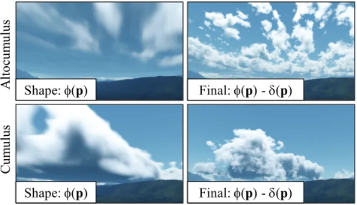
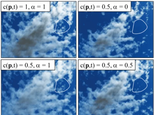
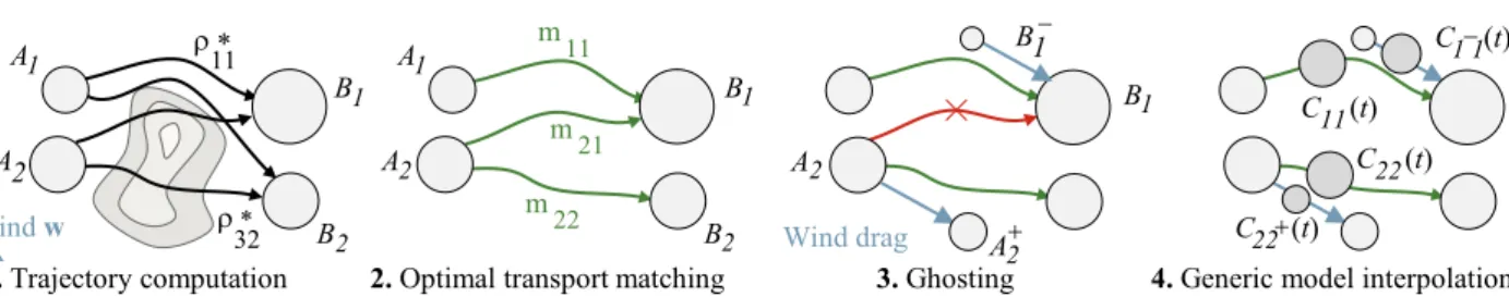
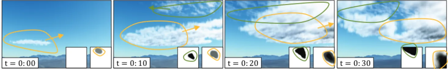
Figure


Documents relatifs
Le soleil avait –il brillé pendant deux jours.. WOULD Action volontaire régulière et répétitive dans
~ 78 Singles: Überraschende neue Studien zeigen, dass Allein- lebende sich zufrieden über Autonomie, Freundeskreis und Gesundheit auBern.. 82 Forschung: Der Psychologe Hans-Werner
determining a certain configuration S in Euclidean n-dimen- sional space; in what cases and by what methods can one pass from the equation to the topological
The Canadian Primary Care Sentinel Surveillance Network, a Pan-Canadian project led by the CFPC that conducts standardized surveillance on selected chronic
suggests a proposed protocol for the ARPA-Internet community, and requests discussion and suggestions for improvements.. 986 Callon Jun 86 Working Draft
The figure describes the process from the perspective of a community working on a single primary protocol suite (such as the IETF/IESG/IAB working on the TCP/IP protocol
Ideally the routing system should allow to shift the overhead associated with a particular routing requirement towards the entity that instigates the requirement (for
On 29 August 2012, the leaders of the IEEE Standards Association, the IAB, the IETF, the Internet Society, and the W3C signed a statement affirming the importance of a
