HAL Id: hal-00318133
https://hal.archives-ouvertes.fr/hal-00318133
Submitted on 9 Aug 2006
HAL is a multi-disciplinary open access
archive for the deposit and dissemination of
sci-entific research documents, whether they are
pub-lished or not. The documents may come from
teaching and research institutions in France or
abroad, or from public or private research centers.
L’archive ouverte pluridisciplinaire HAL, est
destinée au dépôt et à la diffusion de documents
scientifiques de niveau recherche, publiés ou non,
émanant des établissements d’enseignement et de
recherche français ou étrangers, des laboratoires
publics ou privés.
isolated substorms and sawtooth events
X. Cai, C. R. Clauer, A. J. Ridley
To cite this version:
X. Cai, C. R. Clauer, A. J. Ridley. Statistical analysis of ionospheric potential patterns for isolated
substorms and sawtooth events. Annales Geophysicae, European Geosciences Union, 2006, 24 (7),
pp.1977-1991. �hal-00318133�
www.ann-geophys.net/24/1977/2006/ © European Geosciences Union 2006
Annales
Geophysicae
Statistical analysis of ionospheric potential patterns for isolated
substorms and sawtooth events
X. Cai, C. R. Clauer , and A. J. Ridley
Space Physics Research Laboratory, University of Michigan, Ann Arbor, Michigan, USA Received: 12 February 2006 – Accepted: 6 June 2006 – Published: 9 August 2006
Abstract. We present here results which contrast isolated
substorms with individual sawtooth events. Sawtooth events are defined as quasi-periodic, large-amplitude oscillations in the energetic particle flux with a periodicity of 2–4 h ob-served at the geosynchronous orbit. Sawtooth events have several similarities to isolated substorms leading therefore, to different opinions about whether sawtooth events are just an intense periodic form of substorms or if they deserve a category of their own. To help resolve this, we examine the ionospheric potential patterns in the northern polar region for isolated substorms and sawtooth events using the assimilative mapping of ionospheric electrodynamics (AMIE) technique. First we show a statistical analysis of isolated substorm po-tential patterns. In order to examine the seasonal variation, isolated substorms are identified by mid-latitude positive bay in the north-south geomagnetic perturbation in each season, respectively. Superposed epoch analysis (SEA) is applied to obtain the typical polar potential patterns for each season. By examining the time evolution of the potential patterns and cross polar cap potential (CPCP) for isolated substorms during each season, we find only subtle seasonal variations in the results obtained using the AMIE analysis. This pro-vides a basis for comparison with sawtooth events in the next step. From the averaged potential patterns of 213 isolated substorms and those of 184 individual sawtooth events, we find the sawtooth events show signatures similar to subtorms: the DP 1 potential pattern develops and dominates the polar region after the onset. However, the DP 1 potential cell of sawtooth events encompasses a larger area than that of iso-lated substorms. Moreover, the CPCP of sawtooth is stronger than that of isolated substorms. It is also shown that the saw-tooth events displays greater variability between individual events than isolated substorms. We conclude that in terms of ionospheric electrodynamics, the sawtoothe events have fea-tures that are similar to those of isolates substorms, though larger in spatial extent and in magnitude.
Correspondence to: X. Cai ([email protected])
Keywords. Ionosphere (Electric fields and currents) –
Mag-netospheric physics (Electric fields; Storms and substorms)
1 Introduction
The purpose of this paper is to investigate the similarities and differences between isolated substorms and individual sawtooth events by examining the ionospheric electric po-tential patterns in the northern polar region. Sawtooth events are global storm-time phenomena, so named because of the shape of the energetic particle flux measurements at geosyn-chronous orbit. These particle flux data show repetition of slow decreases followed by rapid large amplitude increases (especially clear in the proton flux). The sudden increase in the particle flux following a slow decrease near local mid-night at geosynchronous orbit is normally described as parti-cle injection and is a typical signature of the magnetospheric substorm. For a satellite located inside the injection region the particle injection for all energy channels is observed to occur almost simultaneously which is called a dispersionless injection (Lopez et al., 1990). For sawtooth events, the dis-persionless particle injection is observed with a wider local time range than that of a typical isolated substorm which is confined to near local midnight only. The sawtooth injection region sometimes extends past the dawn and/or dusk termi-nators (Reeves et al., 2002). Meanwhile, the individual saw-tooth event also shows several similarities to substorm signa-tures: auroral observation in the polar region, magnetic dipo-larization at geosynchronous orbit and magnetic perturbation measured by ground magnetometers (e.g., Henderson, 2004; Henderson et al., 2005; Huang, 2002; Huang et al., 2003b; Clauer et al., 2006). An important research issue now con-cerns whether a individual sawtooth event is just an intense form of a magnetospheric substorm or whether it is a new global mode of magnetosphere activity.
Henderson (2004) re-examines the CDAW-9C interval which is a well studied substorm interval, and determines it
to be actually a sawtooth event. This implies that the saw-tooth events were considered as substorms in the past before people used the sawtooth terminology. Investigating the au-roral onset in the polar region, particle injection and geomag-netic field stretching and dipolarization at geosynchronous orbit for each tooth, Henderson concludes that each tooth shows characteristics identical to substorms. However, the geomagnetic perturbation is observed over a wider magnetic local time sector than that during typical isolated substorms. Henderson suggests the sawtooth events represent a mode in which the substorm activity is brought close to the Earth for extended periods of time.
Huang (2002) describes these phenomena as periodic sub-storms. Huang et al. (2003b) apply multiple space-based and ground-based instrumental observations to sawtooth injec-tions and show that the magnetosphere and ionosphere have the similar periodicities. All the observations show corre-spondence with substorm signatures. Further more, Huang et al. (2003c) suggest that magnetospheric substorms have an intrinsic periodicity of 2–3 h, which is unrelated to the varia-tion of exterior solar wind driving condivaria-tions. The sawtooth injections may be initiated by a solar wind pressure pulse impinging on the magnetosphere. The resulting oscillations may continue with the intrinsic periodicity for several cycles when the solar wind and interplanetary magnetic field (IMF) are stable. The sawtooth injections could also be triggered by oscillations in solar wind ram pressure with a changing period comparable to the substorm intrinsic cycle (Huang et al., 2003c).
Lui et al. (2004) examine the magnetotail behavior for 20 April 2002 sawtooth event using GEOTAIL data. They find that the southward dipping, i.e., negative Bz with small dip-ping angle from Sun-Earth line which is a typical feature for substorm expansion phase in the tail lobe magnetic field, does not always coincide with the onset of the sawtooth in-jections. Southward dipping is seen over a wide local time sector which suggests global behavior in the tail lobe. How-ever, the intermittent plasma sheet disturbance is pretty lo-calized which is similar with that of an isolated substorm.
Clauer et al. (2006) examine the mid-latitude magnetic disturbance feature for the same event. They investigate the magnetic local time (MLT) extent of the current wedge. The averaged MLT extent is approximately 7.7 h while the av-eraged local time extent for a typical isolated substorm is about 2.5 h (Clauer and McPherron, 1974b). From this mid-latitude magnetic disturbance feature, it is evident that field-aligned currents (FACs) also form near local midnight dur-ing sawtooth intervals. The difference is the current wedge of sawtooth events has a wider local time width than that of substorm. This agrees with Henderson (2004) and Kitamura et al. (2005). Moreover, Clauer et al. (2006) show that the FACs system for each tooth varies in location, pattern and strength. The width of FACs changes from about 3 h MLT to 12 h MLT.
The statistical study on solar wind driving conditions for sawtooth events by Borovsky et al. (2006)1shows that they occur during strong and steady driving, low magnetosheath mach number and: 1) moderate proton number density and solar wind velocity, 2) steady and strong southward Bz (≤– 10 nT). This implies strong merging electic field and there-fore strong solar wind-magnetosphere coupling in the polar region.
To further understand the relationship between sawtooth events and substorm events, we examine the electrodynamic processes in the high latitude for isolated substorms and in-dividual sawtooth events.
There is a long history of investigating the ground mag-netic perturbations and their associated electric fields for sub-storms in the high latitude region. The electrodynamics pro-cesses are described by introducing equivalent current sys-tems which are assumed as a toroidal horizontal sheet current following in a shell at 110-km altitude. Two equivalent cur-rent systems DP 1 and DP 2 are suggested to be associated with the magnetic perturbations (Nishida, 1968). DP 1 cur-rent system is associated with substorm expansion phase and locates in a narrow latitudal region on the nightside. On the contrary, DP 2 current system could exist during both quiet time and disturbed time and has two cells with one vortex in the morning sector and one in the evening sector (Nishida and Kokubun, 1971).
Clauer and Kamide (1985) separate the two current sys-tems for 22 March 1979 substorm by differential technique. In this technique, they choose a time interval T =T2−T1. By
assuming during the interval T that the current system at T1is
constant while additional current system develops and decays during the same interval, the additional current system is then obtained by subtraction the current system at T1from
subse-quent current system T2. They confirm that DP 2 is evident
before the substorm expansion phase and DP 1 is predom-inant during the expansion phase. They also suggest DP 2 current system is driven by solar wind directly while DP 1 is due to internal magnetospheric process. The two current sys-tems are discussed in more detail by Kamide and Kokubun (1996) and Kamide et al. (1996). They demonstrate that the DP 2 current corresponds the directly driven process that the solar wind energy is deposited into the magnetosphere from dusk and dawn sectors and the DP 1 current corresponds the unloading process that the energy stored the tail in the growth phase releases by forming the westward electrojet in the midnight sector. Moreover, Kamide and Kokubun (1996) show that this two-component auroral electrojet can explain reasonably well several controversial issues about electrody-namic processes of magnetospheric substorms.
1Borovsky, J. E., Nemzek, R. J., Smith, C. W., Skoug, R. M.,
and Clauer, C. R.: The solar wind driving of global sawtooth oscil-lations and periodic substorms: what determines the periodicity?, Ann. Geophys., submitted, 2006.
Figures TRW SJG PST VSS ASC GUI SPT TAM CLF HER TSU FUR BDV NCK THY HRB HBK SUA TAN ABG PHU LRM GNA BMT LNP KNY KDU ASP HTY KAK CBI MMB CTA API HON PPT FRN TUC DLR BSL 50 nT 14 14:26 15 16 17 1999-09-30 14:00:00 - 1999-09-30 17:00:00
Fig. 1. Three hours’ stackplot of X component magnetic perturbation for a typical isolated substorm
on 30 September, 1999. The mid-latitude ground stations are arranged longtitudially with 0◦on the top and 360◦on the bottom. The local time midnight for each station is shown as a triangle. The expansion phase starts at 14:26 UT and arrives its peak at 14:55 UT which are illustrated by vertical dashed lines.
21
Fig. 1. Three hours’ stackplot of X component magnetic
perturba-tion for a typical isolated substorm on 30 September 1999. The mid-latitude ground stations are arranged longtitudially with 0◦on the top and 360◦on the bottom. The local time midnight for each sta-tion is shown as a triangle. The expansion phase starts at 14:26 UT and arrives its peak at 14:55 UT which are illustrated by vertical dashed lines.
In this paper, we investigate the time evolution of iono-spheric potential patterns using the assimilative mapping of ionospheric electrodynamics (AMIE) (Richmond and Kamide, 1988; Richmond, 1992; Ridley and Kihn, 2004) for isolated substorms and individual sawtooth events. We consider the results in terms of the two-component equiva-lent current system DP 1 and DP 2. To investigate seasonal effects in the potential patterns, in the first step, we classify the subtorms events into spring, summer, autumn and winter seasons. The statistical analysis is applied for each season in-dividually. However, we find only small seasonal variations. Therefore in the second step, the averaged ionospheric poten-tial patterns obtained for sawtooth events are then compared with those of isolated substorms to determine the similarities and differences, without regard for seasons.
2 Data and methodology
2.1 Isolated substorm
In this research, isolated substorms are identified based on their mid-latitude feature (Clauer and McPherron, 1974a) from ground magnetometer observations. The method of mid-latitude analysis is described in more detail by Clauer et al. (2003). We use corrected geomagnetic coordinates with the X axis pointing north and Y, Z axes orienting east and ver-tically down respectively. Isolated substorms are identified by positive bays in the X component perturbation measured by stations near local midnight. Local time-universal time (LT–UT) contour maps display the temporal and spatial de-velopment of the magnetic perturbation during the substorm expansion period. Our specific criteria require: 1) positive
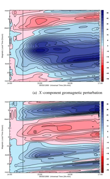
14:00 15:00 16:00 17:00 09/30/1999 Universal Time (hh:mm) noon 15 dusk 21 0 3 dawn 9 noon
Magnetic Local Time (hours)
-12 -12 -12 -4 -4 -4 -4 -4 -4 -4 4 4 4 4 4 4 4 4 4 4 12 12 12 12 12 20 20 20 20 28 28 28 28 36 36 36 36 44 44
(a) X-component geomagnetic perturbation
14:00 15:00 16:00 17:00 09/30/1999 Universal Time (hh:mm) noon 15 dusk 21 0 3 dawn 9 noon
Magnetic Local Time (hours)
-15 -9 -9 -9 -9 -9 -3 -3 -3 -3 -3 -3 -3 -3 -3 -3 -3 -3 3 3 3 3 3 3 3 3 3 3 3 3 3 3 3 3 3 9 9 9 9 9 9 9 9 9 9 15 15 15 15 15 15 21 21 2733
(b) Y -component geomagnetic perturbation
Fig. 2. LT-UT contour maps for X and Y component magnetic perturbations for the same period
showed in Figure 1. Blue and red shaded area mark the positive and negative magnetic perturbation regions. The color bar on the right shows the perturbation strength. The vertical axis shows the magnetic local time with local midnight in the middle and local noon at the top and the bottom. The horizontal axis is the universal time. The onset time of the substorm is illustrated by a vertical black line. To illustrate the development of substorm development, the magnetic perturbation profile at the onset of expansion phase is subtracted from subsequent magnetic perturbation. The inward and outward FACs are marked out in (b).
22
Fig. 2. LT–UT contour maps for X and Y component magnetic
perturbations for the same period showed in Fig. 1. Blue and red shaded area mark the positive and negative magnetic perturbation regions. The color bar on the right shows the perturbation strength. The vertical axis shows the magnetic local time with local midnight in the middle and local noon at the top and the bottom. The hor-izontal axis is the universal time. The onset time of the substorm is illustrated by a vertical black line. To illustrate the development of substorm development, the magnetic perturbation profile at the onset of expansion phase is subtracted from subsequent magnetic perturbation. The inward and outward FACs are marked out in (b).
mid-latitude perturbations in X component LT–UT map near the local midnight; 2) clear FACs in Y component LT–UT map (i.e., clear substorm current wedge) and 3) no pertur-bation at least one hour before the onset time of expansion phase of the substorm.
Figures 1 and 2 show an example of a typical isolated sub-storm. Figure 1 displays the stackplot of X component mag-netic perturbation. After the onset time of expansion phase at 14:26 UT, the magnetic perturbation begins to increase from
100 102 104 106 1990-095 100 102 104 106 1991-080 100 102 104 106 1994-084 100 102 104 106 LANL-97A 0 3 6 9 12 15 18 21 24
Universal Time (hour),1998-09-25
04:21 06:10 08:19 10:05 12:16 14:08 15:58
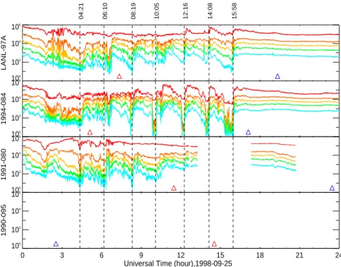
Fig. 3. Proton flux data on September 25, 1998 measured by LANL geosynchronous satellites LANL-97A, 1994-084, 1991-080 and 1990-095 (no data available). The time resolution is 10 sec-onds. For each panel, red line plots lower energy channel and blue higher energy channel. Local noon and local midnight for each satellite are marked by red and blue triangles. The onset for each tooth is illustrated by dashed vertical lines with the onset time shown on the top.
23
Fig. 3. Proton flux data on 25 September 1998 measured by LANL geosynchronous satellites LANL-97A, 1994-084, 1991-080 and 1990-095
(no data available). The time resolution is 10 s. For each panel, red line plots lower energy channel and blue higher energy channel. Local noon and local midnight for each satellite are marked by red and blue triangles. The onset for each tooth is illustrated by dashed vertical lines with the onset time shown on the top.
stations ABG (∼4.5 h before local midnight) to CTA (∼ 0.7 h after the local midnight). This increased perturbation is de-scribed as positive bay which shows the integrated effects from FACs. The magnitude of the perturbation at the peak of expansion phase varies with the location of the station. The maximum increase is measured by station GNA at about 1.7 h before the midnight. The magnitude drops both east-ward and westeast-ward of the GNA. This hints the center of the FACs locates within 2 h pre-midnight. For stations westward of PHU a negative bay is observed to associate with the posi-tive bay. This is attrbuted to the development of an asymmet-ric ring current in the dusk sector. We also notice the peak of the partial ring current is about 2 min earlier than the peak of the current wedge.
Figure 2 displays the X and Y component magnetic pertur-bations spatially and temporally. The magnetic perturbation at the onset time is subtracted as the base perturbation level. The positive bay which is illustrated in blue shaded contours in (a) and the center is between 22 MLT and 23 MLT. The in-ward FAC and outin-ward FAC of the current wedge are shown in red and blue shaded contours in (b). The width of the current wedge can be approximately estimated as the separa-tion of the foci of the perturbasepara-tion cell. Therefore the current wedge is about 6-h MLT wide. Combining the stackplot and the LT–UT contour maps can give a clear picture of the de-velopments of current wedge and FACs during a substorm interval.
To obtain the seasonal features of the isolated substorms, we define each season from 15 days before to 15 days af-ter the equinox/solstice. Using ground magnetic data from 1997–2001, we find 81, 29, 72 and 31 isolated substorms in spring, summer, autumn and winter, respectively.
2.2 Sawtooth events
Sawtooth events are identified from particle flux data ob-tained by the Synchronous Orbit Particle Analyzer (SOPA) instruments installed on LANL geosynchronous satellites. The saw blade shape is more prominent in proton flux data with energy range between 50 keV and 400 keV. The criteria to identify sawtooth events used in this research are: 1) at least one satellite around local noon (±03 MLT h from local noon) and one around local midnight (±03 MLT h from local midnight); 2) the particle injection is observed quasi-globally and quasi-simultaneously.
Here we show in Fig. 3 an example of sawtooth events se-ries on 25 September 1998 to illustrate the general morphol-ogy and the difficulty in determing the onset time for each tooth. Seven tooth intervals are identified. There are sev-eral characteristics worth noting. First, the particle injection is observed with a larger local time range (sometimes even across the dusk and/or dawn terminators, Reeves et al., 2002) than that observed during isolated substorms. At 08:19 UT, LANL-97A is located at around 13:00 MLT, 1994-084 at
100 102 104 106 1990-095 100 102 104 106 1991-080 100 102 104 106 1994-084 100 102 104 106 LANL-97A 14 15 16 17 18 19 20
Universal Time (hour),1998-09-25
14:08 15:54 15:58
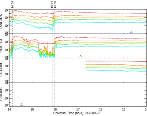
Fig. 4. Proton flux data around 16:00 UT. The two vertical dotted lines mark the onset of dispersion-less injections observed by LANL-97A at 15:54 UT and 1994-084 at 15:58 UT respectively.
24
Fig. 4. Proton flux data around 16:00 UT. The two vertical dotted lines mark the onset of dispersionless injections observed by LANL-97A
at 15:54 UT and 1994-084 at 15:58 UT, respectively.
15:00 MLT and 1991-080 at 09:00 MLT. All three satellites record this particle injection, which means the particle injec-tion is observed from 09 MLT to 15 MLT, including local noon. This is different from the more common particle in-jection during a magnetospheric substorm period, which is confined to local midnight only.
Second, the magnitude of flux increase is different for each satellite. For 12:16 UT particle injection, 1991-080, which is located at 11:00 MLT, observes a flux increase by approxi-mately a factor of 5. However, for satellites LANL-97A and 1994-084 which are located at 17:00 MLT and 19:20 MLT, the proton flux increases by 1 and 2 orders respectively. The flux increase at dusk is larger than the flux increase at noon and the flux increase at post-dusk region is larger than that at predusk region. This can be explained that the injection center is close to the dusk meridian as pointed out by Reeves et al. (2002).
Third, there might be a delay time between the onset of dispersionless particle injections observed by two satel-lites. As shown in Fig. 4, for the last particle injection, LANL-97A, located at 20:40 MLT, observes one disper-sionless injection at 15:54 UT while 1994-084, located at 22:58 MLT, records one dispersionless injection at 15:58 UT. In fact, a precursor smaller amplitude injection is observed around 15:54 UT for 1994-084 satellite. The sudden im-pulse in flux measurement is more complicated than being described as particle injections (Henderson, 2005, personal communication). Other mechanisms with time scale shorter
than the periodicity of sawtooth event can contribute to the particle flux variations.
It is therefore sometimes difficult to decide the onset time of individual sawtooth event. Sometimes, it is possible to utilize additional other data, for example, magnetic dipo-larization from geosynchronous satellites, polar aurora im-age from polar orbiting satellites, and magnetic field mea-surement from GEOTAIL satellites to help identify the on-set time. One disadvantage of those data is that a satellite is not always in the ideal location, for example only part of one period of a polar orbiting satellite is in the polar re-gion. Moreover, there may be a delay time between particle injection phenomenon and other corresponding phenomena observed by satellites since we still do not completely under-stand the whole process. Traditionally, the onset time is de-fined at the earliest time when the rapid proton flux increases are observed by all LANL geosynchronous satellites. In this paper, we follow the tradition method to identify the onset time of individual sawtooth event.
Using proton flux data from January 1997 to September 2003, we find 42 sawtooth intervals which have 184 individ-ual teeth total.
2.3 Statistical analysis metholodogy
We examine the ionospheric electric potential patterns that develop during isolated substorms and individual sawtooth events. These patterns are determined using the AMIE technique to invert the ground magnetometer measurement.
Spring Summer Autumn Winter -8 0 0 8 12 18 0 Min:-27.18 Max:19.39 -40 -20 0 20 40 (kV) -8 0 0 0 0 8 12 18 0 Min:-26.96 Max:23.49 -40 -20 0 20 40 (kV) -8 0 0 0 8 12 18 0 Min:-31.86 Max:22.87 -40 -20 0 20 40 (kV) -8 0 0 0 8 12 18 0 Min:-22.86 Max:20.38 -40 -20 0 20 40 (kV) 0.0 18 5 Min: -2.41 Max: 2.85 5 Min: -1.87 Max: 2.88 0.0 5 Min: -3.07 Max: 3.86 0.0 0.0 06 5 Min: -1.60 Max: 4.55 0.0 18 10 Min: -4.92 Max: 6.34 0.0 10 Min: -3.94 Max: 6.48 0.0 10 Min: -6.10 Max: 8.27 06 10 Min: -4.15 Max: 7.18 0.0 18 15 Min: -6.69 Max: 9.57 0.0 15 Min: -5.15 Max:11.02 0.0 0.0 15 Min: -8.14 Max:12.31 0.0 0.0 06 15 Min: -5.20 Max:10.12 0.0 00 18 20 Min: -8.12 Max:12.39 0.0 0.0 00 20 Min: -5.86 Max:13.48 0.0 0.0 5.0 00 20 Min: -9.49 Max:17.96 0.0 0.0 00 20 Min: -5.46 Max:13.73 -20 -10 0 10 20 (kV)
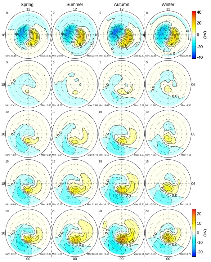
Fig. 5a. The time evolution of the averaged ionospheric residual potential patterns for isolated substorms in each season is shown in column.
From the left to right, we display the potential patterns for spring, summer, autumn and winter respectively. The averaged potential patterns at the onset time of expansion phase for each season which are subtracted as the base are also plotted in the first row. The contour level is 4.0 kV. The patterns are shown every 5 min. Only the potential patterns 45 min after the onset of expansion phase are examined. The contour level is 2.5 kV for the residual potential patterns.
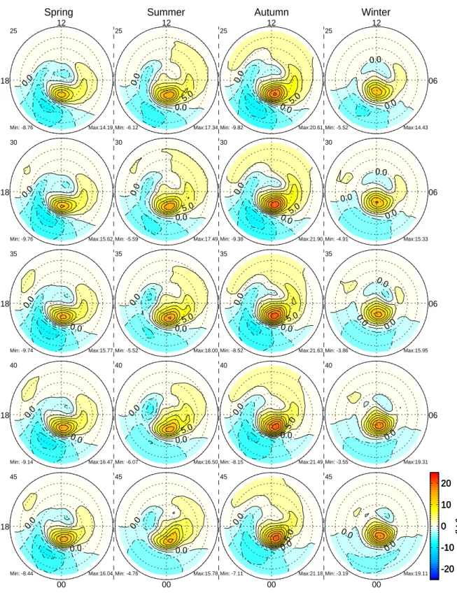
Spring Summer Autumn Winter 0.0 12 18 25 Min: -8.76 Max:14.19 0.0 0.0 5.0 12 25 Min: -6.12 Max:17.34 0.0 0.0 5.0 12 25 Min: -9.82 Max:20.61 0.0 0.0 06 12 25 Min: -5.52 Max:14.43 0.0 18 30 Min: -9.76 Max:15.62 0.0 0.0 5.0 30 Min: -5.59 Max:17.49 0.0 0.0 5.0 30 Min: -9.38 Max:21.90 0.0 0.0 0.0 06 30 Min: -4.91 Max:15.33 0.0 0.0 18 35 Min: -9.74 Max:15.77 0.0 0.0 5.0 35 Min: -5.52 Max:18.00 0.0 0.0 5.0 35 Min: -8.52 Max:21.63 0.0 0.0 0.0 06 35 Min: -3.86 Max:15.95 0.0 0.0 18 40 Min: -9.14 Max:16.47 0.0 0.0 5.0 40 Min: -6.07 Max:16.50 0.0 0.0 5.0 40 Min: -8.15 Max:21.49 0.0 06 40 Min: -3.55 Max:19.31 0.0 0.0 00 18 45 Min: -8.44 Max:16.04 -20 -10 0 10 20 (kV) 0.0 0.0 00 45 Min: -4.76 Max:15.78 -20 -10 0 10 20 (kV) 0.0 0.0 5.0 00 45 Min: -7.11 Max:21.18 -20 -10 0 10 20 (kV) 0.0 0.0 00 45 Min: -3.19 Max:19.11 -20 -10 0 10 20 (kV)
Fig. 5. The time evolution of the averaged ionospheric residual potential patterns for isolated sub-storms in each season is shown in column. From the left to right, we display the potential patterns for spring, summer, autumn and winter respectively. The averaged potential patterns at the onset time of expansion phase for each season which are subtracted as the base are also plotted in the first row. The contour level is 4.0 kV. The patterns are shown every 5 minutes. Only the potential patterns 45 minutes after the onset of expansion phase are examined. The contour level is 2.5 kV for the residual potential patterns.
26
Fig. 5b. Continued.
The background electric potential utilized by AMIE is the Weimer (1996) model which is driven directly by upstream IMF and solar wind conditions. In the inversion process, Hall and Pederson conductance elements are obtained from the measured ground magnetic disturbance using the for-mulation by Ahn et al. (1993, 1998). We use AMIE to invert ground magnetic measurements with supplementary IMF and solar wind data, hemispheric power index (HPI) computed by NOAA to adjust the background potential and conductivity patterns. The time step for AMIE inversion is one minute (Ridley and Kihn, 2004).
A serious concern is the ability of AMIE to globally mea-sure the ionospheric electric field during strom and substorm periods. Using magnetometers data only, one can argue that the potential patterns strongly depend on the ionospheric conductance. It is possible that we may underestimate the the auroral conductance and therefore overestimate the nightside electric field (Kihn and Ridley, 2005). Since there are no good methodologies for measuring the electric field and con-ductance on a global scale during active time periods, this remains a serious source of uncertainty for storm and sub-storm studies. Low-altitude satellites could only measure the potential pattern in its trajectory. Radars can not measure the entire pattern neither and they lose coherence when aurora develops. Therefore given the large number of magnetome-ters, the great IMF coverage and the technique in AMIE to make the data set consistent, the AMIE results are very good for a statistical study. The main purpose of this paper is to examine whether there are significant seasonal differences in the potential patterns of isolated substorms and whether sawtooth events are significantly different than substorms in terms of their electrodynamic properties. Even given all of the uncertainties in AMIE, we have confidence in our con-clusions. Obviously, the subtle aspects of each individual sawtooth and substorm may not be accurately represented by AMIE (using only magnetometer data), but the general char-acteristics are well represented.
As mentioned in the introduction of this paper, there are two current systems contributing to the substorm-time cur-rent structure in the high latitude. Kamide and Kokubun (1996b) shows the two components vary differently during different substorm phases. This is explained more clearly in the sketch plot Fig. 13 in their paper. The DP 1 equiv-alent current system develops and decays while the DP 2 equivalent current system changes. While there is no a spe-cific variation patterns for DP 1 current component, the DP 2 component also varies with the IMF orientation and the cou-pling between the solar wind and the magnetosphere. To obtain an average ionospheric pattern for the isolated sub-storms, we exclude the effects from IMF orientation and cou-pling efficiency between solar wind and magnetosphere, i.e., DP 2 current component. This is accomplished by differen-tial technique (Clauer and Kamide, 1985).
For seasonal substorms, T1 is the onset time of the
ex-pansion phase of each isolated substorm which marks the
sudden increase of the DP 1 current component. We are interested in the development of DP 1 potential pattern af-ter the onset of the expansion phase until the peak of the expansion phase. Kamide and Kroehl (1994) find the typi-cal interval for an isolated substorm is around 120 min: 45 (±22) min in expansion phase and 75 (±32) min in recovery phase. Thus it is reasonable to use 45 min interval in our sta-tistical study. The ionospheric potential pattern at the onset of expansion phase is subtracted from subsequent potential patterns to show the development of the substorm expansion potential patterns (similar to the technique used by Ridley et al.,1997, 1998). These patterns are termed the residual potential patterns 8res. To obtain the average ionospheric potential pattern for isolated substorms, we use a superposed epoch analysis (SEA) methodology. The key time is the on-set of the expansion phase of each isolated substorm. We cal-culate the superposed average over the interval from the pansion onset to 45 min after the onset. In this paper, we ex-amine following characteristics for each season: 1) time evo-lution of residual potential patterns which show the spatial similarities between substorms; and 2) difference between maximum residual potential and minimum residual potential, defined as CPCP∗, which tells the strength of DP 1 potential pattern.
The ionospheric potential patterns for sawtooth events are investigated using the same methodology as seasonal sub-storms. The key time is the onset time of rapid large ampli-tude flux increase from the proton flux data. The interval is 45 min after the onset. The averaged potential patterns are obtained by SEA of the residual potential patterns of all in-dividual teeth and we examine the same set of parameters.
Sawtooth features are compared with those of isolated sub-storms to investigate whether the averaged ionospheric po-tential patterns of sawteeth events are similar with those of isolated substorms or not. As there are only subtle seasonal variations in the patterns for substorms described by AMIE, the averaged residual potential patterns for typical isolated substorms are derived from the all 213 isolated substorms.
3 Results and discussion
3.1 Potential patterns for isolated substorm in each season The time evolution of the substorm expansion phase iono-spheric potential patterns for each season are shown in Fig. 5. As displayed in the first row, the averaged potential pattern at the onset of the expansion phase of each season shows the typical DP 2 potential pattern with a positive potential cell centers in the morning sector and a negative potential cell in the evening sector. This pattern is subtracted from all sub-sequent patterns to isolate the potential pattern that develops during the expansion phase. After the onset, each season shows that DP 1 type potential pattern develops. The DP 1 potential pattern gradually intensifies. There is little seasonal
Spring
0 10 20 30 40
Time after the onset, mins 0 20 40 60 80 100 120 140 Potential, kV Summer 0 10 20 30 40
Time after the onset, mins 0 20 40 60 80 100 120 140 Potential, kV Autumn 0 10 20 30 40
Time after the onset, mins 0 20 40 60 80 100 120 140 Potential, kV Winter 0 10 20 30 40
Time after the onset, mins 0 20 40 60 80 100 120 140 Potential, kV
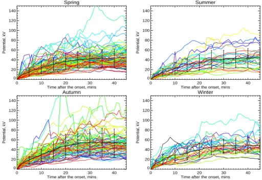
Fig. 6. Summary plot of CP CP∗for each season. In each plot, the CP CP∗for individual isolated substorm is plotted in different color. The mean CP CP∗is plotted as black solid lines. The error bars shows the standard deviation every 5 minutes.
27
Fig. 6. Summary plot of CPCP∗for each season. In each plot, the CPCP∗for individual isolated substorm is plotted in different color. The mean CPCP∗is plotted as black solid lines. The error bars shows the standard deviation every 5 min.
Spring 0 20 40 60 80 100 120 CPCP, kV 0 5 10 15 20 25 30 % of event t=30 Mean : 42.14 kV Stddev : 16.44 kV Ratio : 0.39 Summer 0 20 40 60 80 100 120 CPCP, kV 0 5 10 15 20 25 30 % of event t=30 Mean : 40.60 kV Stddev : 18.77 kV Ratio : 0.46 Autumn 0 20 40 60 80 100 120 CPCP, kV 0 5 10 15 20 25 30 % of event t=30 Mean : 54.55 kV Stddev : 26.80 kV Ratio : 0.49 Winter 0 20 40 60 80 100 120 CPCP, kV 0 5 10 15 20 25 30 % of event t=30 Mean : 47.33 kV Stddev : 14.59 kV Ratio : 0.31
Fig. 7. The distribution of CP CP∗at 30 minutes after the onset of the expansion phase for each season. The numbers of events in each season are 81, 29, 72 and 31, respectively. The bin size is 5 kV for each season. In each plot, the mean value, the standard deviation and the ratio of the standard deviation over the mean values for each season are shown at the right top of each plot.
28
Fig. 7. The distribution of CPCP∗at 30 min after the onset of the expansion phase for each season. The numbers of events in each season are 81, 29, 72 and 31, respectively. The bin size is 5 kV for each season. In each plot, the mean value, the standard deviation and the ratio of the standard deviation over the mean values for each season are shown at the right top of each plot.
variation in the isolated sustorm expansion electric poten-tial patterns except the positive cell for autumn substorms may be slightly more intense. Though we concentrate on the positive DP 1 potential cell at high latitude near local mid-night, it is also interesting to notice the development of the
large negative potential cell around 55◦latitude premidnight. The pattern is very similar to the penetration electric poten-tial pattern well modeled by Ridley and Liemohn (2002). Though they simulate the penetration electric field in storm time, the source of the electric field is due to the divergence
-5.0 -5.0 0.0 0.0 0.0 5.0 12 18 Sub. 1 Min:-10.27 Max:14.64 -5.0 0.0 0.0 5.0 10.0 06 12 Sub. 2 Min:-16.23 Max:21.36 -10.0 -5.0 0.0 0.0 0.0 5.0 10.0 00 18 Sub. 3 Min:-16.78 Max:23.83 -5.0 0.0 0.0 5.0 00 Ave. Min: -9.00 Max:18.13 -20 -10 0 10 20 (kV)
Fig. 8. A example shows the distribution of the residual potential pattern at a specific time for three
isolated substorms and the averaged pattern of them at the same time. The maximum and minimum
potential for each plot are shown in the left and right bottom corner. The difference of these two are
CP CP
∗. The contour level is 2.5 kV.
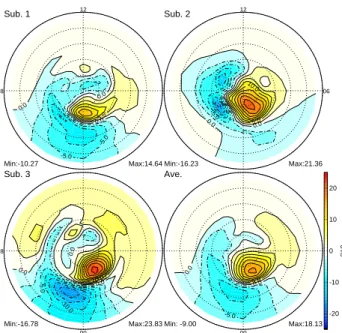
Fig. 8. An example shows the distribution of the residual
poten-tial pattern at a specific time for three isolated substorms and the averaged pattern of them at the same time. The maximum and min-imum potential for each plot are shown in the left and right bottom corner. The difference of these two are CPCP∗. The contour level is 2.5 kV.
of the asymmetric ring current which also develops in sub-storm time. So a similar pattern should be expected during magnetospheric substorm. We find the negative potential cell is slightly stronger in equinox than in solstice which could be as a result of the seasonal variation in the conductance pat-tern. Ebihara et al. (2004) show there is a large difference in Pederson conductance between in equinox and in solstice. Their simulated Dst∗ shows evident semiannual variation that Dst∗is stronger in equinox than in solstice. Our results agree with this.
We can infer the strength of DP 1 potential cell from the CPCP∗ plotted in Fig. 6. To make it easy to compare, the plot ranges of Y axis are the same. For all seasons, the CPCP∗increases gradually after the expansion phase of each substorm and approaches a steady value. This means the DP 1 cell develops and stays relatively steady in the polar region. A possible reasons we do not see CPCP∗ decrease is that we only show CPCP∗ for 45 min after the onset of expansion phase, thus we do not continue into the recov-ery phase. Moreover, the CPCP∗for all seasons except for autumn increase by about 40 kV in 30 min after the onset. The mean CPCP∗for autumn substorms increases by 55 kV which is larger than other seasons. This difference is prob-ably due to a small number of autumn substorms with high CPCP∗. Then it is necessary to examine the distribution of CPCP∗ at a certain time for all seasonal substorms which will be discussed next.
The distributions of the CPCP∗ for each season 30 min after the onset of expansion phase are plotted in Fig. 7. The CPCP∗for most of events in each season is around 40 kV. For winter substorms, the peak is seen around 35 kV which is probably due to slightly larger uncertainty in conductance than other seasons. Overall, the distributions imply the DP 1 potential cell has approximately the same strength for most of substorms in all seasons.
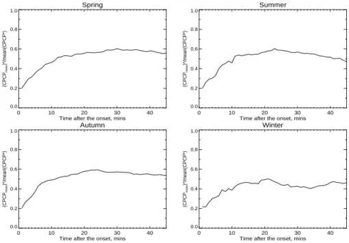
The consistency between substorms can be examined by plotting the ratio of the CPCP∗ of the super-posed epoch combined residual potential patterns to the mean values of CPCP∗for all substorms. The basic idea is when all poten-tial patterns are combined together the individual features are obviously lost. To illustrate this, we give one simple exam-ple in Fig. 8. For the potential patterns of the three isolated substorms, it is evident that there is a positive DP 1 poten-tial cell around midnight and one negative potenpoten-tial cell in subaurora region premidnight. However, the center for the DP 1 potential cell slightly differs from one to another. The CPCP∗for each event are 24.9 kV, 37.6 kV and 40.6 kV re-spectively. So the averaged CPCP∗is 34.4 kV. Though in the averaged distribution of potential patten, we still can clearly see the DP 1 potential cell and subauroral negative cell how-ever the details in individual event are missing. For example, the negative potential cell around local noon in the first sub-storm and the one before the dusk in the second subsub-storm are no longer prominent in the averaged pattern. Similarly, the dayside elongated positive cell with potential between 2.5 kV to 5.0 kV in the third substorm become under 2.5 kV in the averaged pattern. Moreover, the shape of the DP 1 potential cell in the averaged pattern follows none of the shape of the DP 1 potential cell in individual event. The CPCP∗ of the averaged pattern is 27.1 kV which is smaller than the mean CPCP∗of three substorms. The consistency of these three potential patterns is 0.78, which is the ratio of 27.1 to 34.4. However, if all the potential patterns for the three substorms are identical, the CPCP∗of the averaged pattern should ex-actly equal to the mean CPCP∗ of all substorms. There-fore the ratio of the CPCP∗of the averaged pattern over the mean CPCP∗of all substorms would be 1. In reality, the ra-tio is less than 1 due to differences in potential strength at a specific location and in spatial distribution of potential pat-terns between the substorms. In other words, the ratio shows the consistency of the events. The ratios for each season are shown in Fig. 9. For isolated subtorms in spring, summer and autumn, the ratio is greater than 0.5 about 10 min after the onset time. The maximum ratio is about 0.6. Therefore the substorms in these seasons have the same level of con-sistency, or in other words, the same level of variability. For winter substorms, the ratio is slightly smaller than other sea-sons. The ratio is around 0.45 with the peak value 0.5. As mentioned before, in AMIE we might underestimate the au-roral conductance. In winter times, the auau-roral conductance is more important than during other seasons. The uncertain-ties in conductance data also bring uncertainuncertain-ties in potential
Spring
0 10 20 30 40
Time after the onset, mins
0.0 0.2 0.4 0.6 0.8 1.0 (CPCP mean )*/mean(CPCP*) Summer 0 10 20 30 40
Time after the onset, mins
0.0 0.2 0.4 0.6 0.8 1.0 (CPCP mean )*/mean(CPCP*) Autumn 0 10 20 30 40
Time after the onset, mins
0.0 0.2 0.4 0.6 0.8 1.0 (CPCP mean )*/mean(CPCP*) Winter 0 10 20 30 40
Time after the onset, mins
0.0 0.2 0.4 0.6 0.8 1.0 (CPCP mean )*/mean(CPCP*)
Fig. 9. Ratio of the CP CP∗of the averaged potential patterns to the mean values of the CP CP∗ of all substorms for each season.
30
Fig. 9. Ratio of the CPCP∗of the averaged potential patterns to the mean values of the CPCP∗of all substorms for each season.
patterns that decrease the consistency for winter time isolated substorms.
Utilizing SEA methodology on the residual potential pat-terns determined from AMIE, we find there are only subtle seasonal variations in the DP 1 potential pattern developing during the expansion phase of isolated substorms. Overall, the potential patterns from AMIE inversion technique for all seasonal substorms show similar patterns. It is possible to derive typical potential patterns for isolated substorms that can be used for comparison with sawtooth events in the next step.
3.2 Potential patterns for sawtooth events
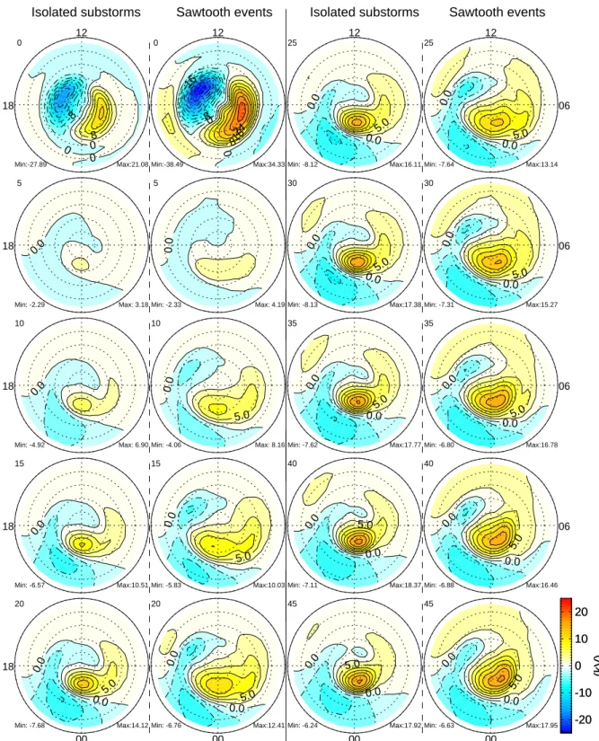
The evolution of the averaged potential patterns for sawtooth events and isolated substorms are plotted in Fig. 10. The potential pattern of a sawtooth event at the onset time dis-plays a DP 2 potential pattern similar with that of an iso-lated substorm. The development of the DP 2 positive poten-tial cell in the morning sector and the negative potenpoten-tial cell in the evening sector during sawtooth events are similar but stronger than those during isolated substorms.
As shown in Fig. 10, the residual potentials show the de-velopment of a DP 1 potential cell near local midnight after the onset of the events at about the same latitude for both isolated substorms and sawtooth events. The DP 1 pattern grows stronger slowly while the spatial region remains sta-tionary. Approximately 25 min later, the DP 1 potential pat-tern dominates the evening sector. Overall, the DP 1 poten-tial pattern development in substorms and sawtooth events is similar. However, there are small differences. The DP 1
pat-tern for sawtooth events encompasses a slightly larger spa-tial area than that of substorms. Moreover, there is a neg-ative cell in the afternoon sector for sawtooth events. This might be due to large intensification of DP 2 pattern after the onset of events and the assumption of differential technique (Clauer and Kamide, 1985) breaks down. More sophisticated methods such as the method of natural orthogonal compo-nents (MNOC) (Sun et al., 1998; 2000) may be necessary to fully decouple the DP 1 potential pattern and the DP 2 potential pattern during sawtooth periods. It is also inter-esting to notice that the negative potential cell at subauroral latitude premidnight (Ridley and Liemohn, 2002; Foster and Burke, 2002) during sawtooth event shows about the same strength as that during a substorm, i.e., the penetration elec-tric field (Ridley and Liemohn, 2002) or subs-auroral polar-ization streams (SAPS) (Foster and Burke, 2002) is of the same strength during both cases.
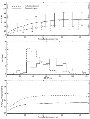
The residual potential CPCP∗showing the average level of the DP 1 potential pattern strength for isolated substorms and individual sawtooth events is plotted as dashed lines and solid lines respetively in the top panel of Fig. 11. Both of the mean trends show increase after the onset time, which implies that DP 1 potential pattern develops in both cases. However, the mean CPCP∗ of sawtooth events are larger than that of substorms indicating the DP 1 potential cell is stronger. At 30 min after the onset, the mean CPCP∗ for individual sawtooth events is 70 kV where that for isolated substorms is about 45 kV. Here CPCP∗is the cross potential cap potential for the residual potential patterns – DP 1 po-tential patterns - with the popo-tential patterns at the onset time removed as the background. Statistical study by (Nagatsuma,
Isolated substorms Sawtooth events Isolated substorms Sawtooth events -8 0 0 0 8 12 18 0 Min:-27.89 Max:21.08 -16 -80 0 816 24 12 0 Min:-38.49 Max:34.33 0.0 18 5 Min: -2.29 Max: 3.18 0.0 5 Min: -2.33 Max: 4.19 0.0 18 10 Min: -4.92 Max: 6.90 0.0 5.0 10 Min: -4.06 Max: 8.16 0.0 18 15 Min: -6.57 Max:10.51 0.0 5.0 15 Min: -5.83 Max:10.03 0.0 0.0 5.0 00 18 20 Min: -7.68 Max:14.12 0.0 0.0 5.0 00 20 Min: -6.76 Max:12.41 0.0 0.0 5.0 12 25 Min: -8.12 Max:16.11 0.0 0.0 5.0 06 12 25 Min: -7.64 Max:13.14 0.0 0.0 5.0 30 Min: -8.13 Max:17.38 0.0 0.0 5.0 06 30 Min: -7.31 Max:15.27 0.0 0.0 5.0 35 Min: -7.62 Max:17.77 0.0 0.0 5.0 06 35 Min: -6.80 Max:16.78 0.0 0.0 5.0 40 Min: -7.11 Max:18.37 0.0 0.0 5.0 06 40 Min: -6.88 Max:16.46 0.0 0.0 5.0 00 45 Min: -6.24 Max:17.92 -20 -10 0 10 20 (kV) 0.0 0.0 5.0 00 45 Min: -6.63 Max:17.95 -20 -10 0 10 20 (kV)
Fig. 10. The time evolution of the averaged ionospheric residual potential patterns for isolated substorms and individual sawtooth events are shown side-by-side. The two columns separated by a solid vertical line in the middle display the time evolution patterns. The averaged potential patterns at the onset time which are subtracted as the base are also plotted. The contour level is 4.0 kV. The residual patterns are shown every 5 minutes. Only the potential patterns 45 minutes after the onset
Fig. 10. The time evolution of the averaged ionospheric residual potential patterns for isolated substorms and individual sawtooth events
are shown side-by-side. The two columns separated by a solid vertical line in the middle display the time evolution patterns. The averaged potential patterns at the onset time which are subtracted as the base are also plotted. The contour level is 4.0 kV. The residual patterns are shown every 5 min. Only the potential patterns 45 min after the onset are examined. The contour level is 2.5 kV.
2002) shows during the strong solar wind drivers with merg-ing electric field higher than 5 mV/m (or a Bzof 12.5 nT) the polar cap potential tends to be saturated. During the sawtooth events when the solar wind driver is strong (Borovsky et al., 2006), the saturation is expected to occur. However, how the DP 1 potential pattern couples with DP 2 pattern and how the saturation occur are still unknown. The standard devi-ation for isolated substorms is smaller than that of sawtooth events suggesting that isolated substorms are more consistent than sawtooth events. Moreover, there is overlap between the CPCP∗ profiles for individual sawtooth events and CPCP∗ profiles for isolated substorms which suggests that some in-dividual sawtooth events are just magnetic substorms.
The distribution of CPCP∗ for sawtooth events and iso-lated substorms at 30 min after the onset time are examined in the middle panel in Fig. 11. The peak of the CPCP∗ distribu-tion for sawtooth events is about 70 kV whereas the substorm peak is around 35 kV. On the other hand, the distribution for sawtooth events spreads out over a broader range, which im-plies the sawtooth events are more variable than substorms.
To examine variability between the events, we plot the ra-tio of the CPCP∗of the averaged pattern to averaged CPCP∗ of all isolated substorms and all sawtooth events in the bot-tom panel in Fig. 11. As mentioned in Sect. 3.1, the CPCP∗ of the averaged pattern is different from the mean CPCP∗ of the residual patterns of the three events. This is due to the spatial distribution difference and the potential strength difference between the events. Therefore the ratio of the CPCP∗of the averaged pattern over the mean CPCP∗of all events can be used to examine the consistency between the events. As shown in Fig. 11., the ratios for isolated substorms are much higher than those of sawtooth events. The ratio for the isolated substorms reaches a level larger than 0.5 after 13 min of the onset time. For sawtooth events, the ratio is never higher than 0.35. Most of time, the ratio is around 0.3. It is evident that isolated substorms show more consistency in DP 1 potential pattern between each other than sawtooth events do.
From the SEA of the potential patterns, we find that the sawtooth events show similar signatures with substorm, i.e., DP 1 potential pattern develops and dominates the local mid-night region. However, for sawtooth events, the DP 1 cell en-compasses a slightly larger area than in isolated substorms. For the SEA of CPCP∗, the mean trend of sawtooth in-creases by 70 kV at 30 min after the onset time while that of the isolated substorm only by 35 kV. Moreover, individ-ual sawtooth events also show larger variability than isolated substorms do.
4 Conclusions
To help to answer if a sawtooth event is just an intense form of substorm or not, this paper analyzes the statistical
char-0 10 20 30 40
Time after the onset, mins 0 20 40 60 80 100 120 140 CPCP, kV Isolated substorms Sawtooth events 0 10 20 30 40
Time after the onset, mins 0.0 0.2 0.4 0.6 0.8 1.0 (CPCP mean )*/mean(CPCP*) 0 20 40 60 80 100 120 CPCP, kV 0 5 10 15 20 % of event
Fig. 11. The summary plots for isolated substorms shown in dashed lines and individual sawtooth
evnets in solid lines. The top panel is the mean CP CP∗with the standard devidation error bars. The middle panel is the histogram of the CP CP∗at 30 minutes after the onset. The bin size is 5 kV for both cases. The bottom figure is the ratio of CP CP∗of averaged potential patterns to the mean values of CP CP∗for isolated substorms and individual sawtooth events.
32
Fig. 11. The summary plots for isolated substorms shown in dashed
lines and individual sawtooth evnets in solid lines. The top panel is the mean CPCP∗with the standard devidation error bars. The middle panel is the histogram of the CPCP∗ at 30 min after the onset. The bin size is 5 kV for both cases. The bottom figure is the ratio of CPCP∗of averaged potential patterns to the mean values of CPCP∗for isolated substorms and individual sawtooth events.
acteristics of the high latitude potential patterns for sawtooth events and isolated substorms.
We utilize the assimilative mapping of ionospheric electro-dynamics to conduct this study. Each inversion of AMIE uses approximately 150 magnetometers, which covers a signifi-cant portion of the high-latitude region. While some events do not have great coverage over the region of interest, and may have high uncertainty, by averaging a large number of events together, a better understanding of the general behav-ior of both isolated substorms and sawtooth events can be gained. It must be understood that there is uncertainty in any technique that attempts to examine the global electric poten-tial pattern. Averaging events together helps to reduce this uncertainty, if there is indeed a systematic behavior or con-sistency. We find that this systematic behavior does exist for isolated substorms, and the sawtooth events as well but the sawtooth events show more variability event to event.
The statistical analysis of the potential patterns for iso-lated substorms and their seasonal variance are discussed in detail first. The isolated magnetospheric substorms are
identified using mid-latitude positive bay signature in the X component magnetic disturbance field. The substorms are categorized into four seasons to investigate if there are sea-sonal variations in the ionospheric pattern. Utilizing SEA methodology on the residual potential patterns determined from AMIE, we find that only subtle seasonal variations in the DP 1 potential pattern developing during the expansion phase of isolated substorms. For all substorms in the four seasons, DP 1 potential patterns develop and gradually dom-inate the nightside polar region after the onset of the expan-sion phase of substorms. Moreover, the most probable po-tential strength CPCP∗for all seasons is approximately the same. The CPCP∗increases by around 35 kV 30 min after the onset.
We also investigate the consistency between substorms for each season. From the ratios for the four season, we find the substorms in spring, summer and autumn have the same consistency. The ratio for winter time substorms is slightly smaller than other seasons. The uncertainty in the conduc-tance in the winter time is larger than other season, which may decrease the consistence.
Overall, the potential patterns from AMIE inversion tech-nique for all seasonal substorms show similar patterns. It is possible to derive typical potential patterns for isolated sub-storms that can be used for comparison with other substorm-like magnetospheric phenomena.
Second, we compare the averaged potential patterns for isolate substorms and sawtooth events. We find that the sawtooth events show similar signatures with substorm, i.e.,
DP1 potential pattern develops and dominates the local mid-night region. However, for sawtooth events, the DP 1 cell encompasses a slightly larger area than in a substorm. For the SEA of CPCP∗, the mean trend of sawtooth increases by 70 kV at 30 min after the onset time while that of the sub-storm only by 35 kV.
Though we emphasize the statistical characteristics of sawtooth events, we also realize that each single tooth still has its own characteristics, for example, the spatial distri-bution of the DP 1 potential cell, the CPCP∗ of the DP 1 potential cell and the details in the ionospheric potential pat-terns. Comparing the charcteristics with those of substorms, we find that the sawtooth events tend to be more diverse. This hints that there may be multiple mechanisms to cause indi-vidual teeth in a sawtooth interval.
Acknowledgements. We great fully acknowledge SPIDR data base
for providing ACE, HPI, Kp data and the Los Alamos National Laboratory for providing SOPA energetic particle data. Magne-tometer data were obtained from DMI, NGDC of NOAA, WDC, 210 Magnetic Meridian Observation Group, INTERMAGNET, IZMIRAN database of Russian Observatories, British Antarctica survey, MACCS, IMAGE, and CANOPUS. This research was sup-ported by NASA Grant NAG5-12176 and NSF Grant OPP0220735. Topical Editor I. A. Daglis thanks C. Huang and another referee for their help in evaluating this paper.
References
Ahn, B.-H., Robinson, R. M., Kamide, Y., and Akasofu S.-I.: Elec-tric conductivities, elecElec-tric fields and auroral particle energy in-jection rate in the auroral ionosphere and their empirical relations to horizontal magnetic disturbances, Planet. Space Sci., 31(6), 641–653, 1983.
Ahn, B.-H., Richmond, A. D., Kamide, Y., Kroehl, H. W., Emery, B. A., de la Beaujardi´ere, O. and Akasofu, S.-I.: An ionospheric conductance model based on ground magnetic disturbance data, J. Geophys. Res., 103(A7), 14 769–14 780, 1998.
Clauer, C. R. and Kamide, Y.: DP 1 and DP 2 current systems for the March 22, 1979 substorms, J. Geophys. Res., 90, 1 343– 1 354, 1985.
Clauer, C. R. and McPherron, R. L.: Mapping the local time – universal time development of magnetospheric substorms using mid-latitude magnetic observations, J. Geophys. Res., 79(19), 2 811–2 820, 1974a.
Clauer, C. R. and McPherron, R. L.: Variability of mid-latitude magnetic parameters used to characterize magnetospheric sub-storms, J. Geophys. Res., 79(19), 2 898–2 900, 1974b.
Clauer, C. R., Liemohn, M. W., Kozyra, J. U., and Reno, M. L.: The relationship of storms and substorms determined from mid-latitude ground-based magnetic maps, in: Disturbaces in Geospace: The Storm – Substorm Relationship, edited by: Sharma, A. S., Kamide, Y., and Lakhina, G. S., AGU, Wash-ington, D.C., 143–157, 2003.
Clauer, C. R., Cai, X., Welling, D., DeJong, A., and Henderson, M. G.: Characterizing the 18 April 2002 storm-time sawtooth events using ground magnetic data, J. Geophys. Res., 111, A04S90, doi:10.1029/2005JA011099, 2006.
Ebihara, Y., Fok, M.-C., Wolf, R. A., Immel, T. J., and Moore, T. E.: Inflence of ionospheric conductivity on the ring current, J. Geophys. Res., 109, A08025, doi:10.1029/2003JA010351, 2004. Foster, J. C. and Burke, W. J.: SAPS: A new characterization for subauroral electric fields, EOS AGU Trans., 83, 393–394, 2002. Henderson, M. G.: The May 2–3, 1986 CDAW-9C in-terval: A sawtooth event, Geophys. Res. Lett., 31(11), doi:10.1029/2004GL019941, 2004.
Henderson, M. G., Reeves, G. D., Skoug, R., Thomsen, M. F., Denton, M. H., Mende, S. B., Immel, T. J., Brandt, P. C., and Singer, H. J.: Magnetospheric and Auroral Activity During The April 18, 2002 Sawtooth Event, J. Geophys.Res., 111(A1), doi:10.1029/2005JA011111, 2006.
Huang, C. S.: Evidence of periodic (2-3 hour) near-tail magnetic re-connection and plasmoid formation: Geotail observations, Geo-phys. Res. Letter., 29(24), doi:10.1029/2002GL016162, 2002. Huang, C. S., Foster, J. G., Reeves, G. D., Le, G., Frey, H. U.,
Pol-lock, C. J., and John, J.-M.: Periodic magnetospheric substorms: Multiple space-based and ground-based instrumental observa-tion, J. Geophys. Res., 108(A11), doi:10:1029/2003JA009992, 2003b.
Huang, C. S., Reeves, G. D., Borovsky, J. E., Skoug, R. M., Pu, Z. Y., and Le, G.: Periodic magnetospheric substorms and their re-lationship with solar wind variations, J. Geophys. Res., 108(A6), doi:10.1029/2002JA009704, 2003c.
Kamide, Y. and Kokubun, S.: Two-component auroral electroject: Importance for substorm studies, J. Geophys. Res., 101(A6), 13 027–13 046, 1996.
Kamide, Y. and Kroehl, H. W.: Auroral electrojet activity during isolated substorms at different local times: A statistical study, Geophys. Res. Lett., 21(5), 389–392, 1994.
Kamide, Y., Sun, W., and Akasofu, S.-I.: The average ionospheric electrodynamics for the different substorm phases, J. Geophys. Res., 101(A1), 99–110, 1996.
Kihn, E. A. and Ridley, A. J.: A statistical analysis of the assimila-tive mapping of ionospheric electrodynamics auroral specifica-tion, J. Geophys. Res., 110, doi:10.1029/2003JA010371, 2005. Kitamura, K., Kawano, H., Ohtani, S., Yoshikawa, A., and
Yu-moto, K.: Local time distribution of low and middle latitude ground magnetic disturbances at sawtooth injections of 18–19 April 2002, J. Geophys. Res., 110, doi:10.1029/2004JA010734, 2005.
Lui, A. T. Y., Hori, T., Ohtani, S., Zhang, Y., Zhou, X. Y., Hen-derson, M. G., Mukai, T., Hayakawa, H., and Mende, S. B.: Magnetotail behavior during storm time “sawtooth injections”, J. Geophys. Res., 109, doi:10.1029/2004JA010543, 2004. Lopez, R. E., Sibeck, D. G., McEntire, R. W., and Krimigis, S. M.:
The energetic ion substorm injection boundary, J. Geophys. Res., 95, 109–117, 1990.
Nagatsuma, T.: Saturation of polar cap potential by intense so-lar wind electric fields, Geophys. Res. Lett., 29(10), 1422, doi:10.1029/2001GL014202, 2002.
Nishida, A.: Geomagnetic DP 2 fluctuations and associated magne-tospheric phenomena, J. Geophys. Res., 73, 1 795–1 803, 1968. Nishida, A. and Kokubun, S.: New polar magnetic disturbances,
Sqp, SP , DP C, DP 2, Rev. Geophys. and Space Physics, 9(2), 417–425, 1971.
Reeves, G. D., Thomsen, M. F., Henderson, M. G., Skoug, R. M., Borovsky, J. E., Jahn, J.-M., Pollock, C. J., Mitchell, D. G., Brandt, P. C., and Mende, S. B.: Global “Sawtooth” activity in the April 2002 geomagnetic storm, Eos Trans. AGU, 83(47), Fall Meet. Suppl., Abstract SA12A-05, 2002.
Richmond, A.: Assimilative mapping of ionospheric electrodynam-ics, Adv. Space Res., 12(6), 59–68, 1992.
Richmond, A. D. and Kamide, Y.: Mapping electrodynamic fea-tures of the high-latitude ionospheree from localized observa-tions: Techinique, J. Geophys. Res., 93, 5 741–5 759, 1988. Ridley, A. and Kihn, E. A.: Polar cap index comparisons with amie
cross polar cap potential, electric field, and polar cap area, Geo-phys. Res. Lett., 31, doi:10.1029/2003GL019113, 2004. Ridley, A. and Liemohn, M. W.: A model-derived storm time
asym-metric ring current driven eletric field description, J. Geophys. Res., 107(A8), doi:10.1029/2001JA000051, 2002.
Ridley, A., Lu, G., Clauer, C. R., and Papitashvili, V. O.: Iono-spheric convection during nonsteady interplanetary magnetic field conditions, J. Geophys. Res., 102(A7), 14 563–14 580, 1997.
Ridley, A., Lu, G., Clauer, C. R., and Papitashvili, V. O.: A statis-tical study of the ionospheric convection response to changing interplanetary magnetic field conditions using the assimilative mapping of ionospheric electrodynamics technique, J. Geophys. Res., 103(A3), 4 023–4 040, 1998.
Sun, W., Xu, W.-Y., and Akasofu, S.-I.: Mathematical separation of directly driven and unloading components in the ionospheric equivalent currents during substorms, J. Geophys. Res., 103(A6), 11 695–11 700, 1998.
Sun, W., Xu, W.-Y., and Akasofu, S.-I.: An improved method to deduce the unloading component for magnetospheric substorms, J. Geophys. Res., 105(A6), 13 131–13 140, 2000.