Effect of information in Bayesian congestion games

Effect of Information in Bayesian Congestion Games

by

Manxi Wu

B.S. Applied Mathematics

Peking University, 2015

Submitted to the Department of Civil and Environmental Engineering

in partial fulfillment of the requirements for the degree of

Master of Science in Transportation

at the

MASSACHUSETTS INSTITUTE OF TECHNOLOGY

June 2017

@

2017 Manxi Wu. All rightes reserved.

The author hereby grants to MIT permission to reproduce and to

distribute publicly paper and electronic copies of this thesis document

in whole or in part in any medium now known or hereafter created.

A uthor ...

Certified by.

Signature redacted

Department of Civil and Environmental Engineering

May

19th. 2017

...

Sina

ur

re dacte

9d...

Saurabh Amin

Assistant Professor of Civil and Environmental Engineering

-

?esis Supervisor

Accepted by ...

JUN 14 2017

LIBRARIES

Signature redacted...

\

Jesse Kroll

Professor of Civil Id Environmental Engineering

Chair, Graduate Program Committee

MITLibranes

77 Massachusetts Avenue

Cambridge, MA 02139

http://Iibraries.mit.edu/ask

DISCLAIMER NOTICE

Due to the condition of the original material, there are unavoidable

flaws in this reproduction. We have made every effort possible to

provide you with the best copy available.

Thank you.

The images contained in this document are of the

best quality available.

Effect of Information in Bayesian Congestion Games

by

Manxi Wu

Submitted to the Department of Civil and Environmental Engineering on May 19th. 2017, in partial fulfillment of the

requirements for the degree of Master of Science in Transportation

Abstract

This thesis studies routing in a general single o-d network and information structure induced by any two heterogeneous information systems. To model the asymmetric information environment, we formulate a Bayesian congestion game, where travelers subscribing to one information system is seen as one population. We study properties of Bayesian Wardrop Equilibrium, where each population assigns their demand to routes with the lowest expected cost based on their belief. We show that if population beliefs about the state and the signal received by the other population are based on a common prior, as the population sizes change, qualitative properties of equilibrium strategies change, resulting in three distinct regimes. In the intermediate regime, the equilibrium edge load does not vary with the relative population size, and both populations face identical cost in equilibrium. In the other two regimes, the "minor" population has lower cost in equilibrium. We also introduce a metric to evaluate the impact of information. The relative population size effects the equilibrium outcome (edge load, costs) if and only if the impact of information on either population is tightly bounded by its size. Finally, we compute the bounds on the equilibrium social cost, and provide a sufficient condition for the bounds to be tight. Although we consider a more general information environment, the worst case inefficiency of equilibrium is the same as that in complete information games.

Thesis Supervisor: Saurabh Amin

Acknowledgments

First and foremost, I would like to express my sincere gratitude to my advisor, Pro-fessor Saurabh Amin, for the continuous support of my study and research. I have benefited greatly from his knowledge, exceptional view of research and life wisdom. It is an honor to be advised by Prof. Amin.

Besides my advisor, I would like to thank Prof. Asuman Ozdaglar for teaching me game theory and providing useful feedback and insightful comments during our meetings. Additionally, I thank Prof. John Tsitsiklis for teaching me probability and optimization, and for discussion of research in several occasions.

I am also grateful to Roberta Pizzinato for her kindness and her help regarding the administrative formalities. I would like to acknowledge the financial support of FORCES (Foundations Of Resilient CybEr-Physical Systems), which receives support from the National Science Foundation (NSF award numbers 1238959,

CNS-1238962, CNS-1239054, CNS-1239166) and NSF CAREER award CNS-1453126.

Many thanks go to my labmates Devendra Shelar, Derek Chang, Li Jin, Mathieu Dahan, Jeff Liu, Zaid Khan and Andrew Lee for intellectual discussions and support. Additionally, I am grateful for my friends, Tianli Zhou, Linsen Chong, Haizheng Zhang, Yiling Xie, Weitong Liu, Xinhao Li, Jiayue Wang and Hongzhou Ye for making

my life at MIT enjoyable and fulfilling.

Most importantly, I would like to thank my parents, Qing Yang and Zhengqiu

Wu, as well as my boyfriend, Chao Wu, for the love, support and understanding. You

Contents

1 Introduction 13

1.1 Overview of the Problem . . . . 13

1.2 Related W ork ... . 14

1.3 Main Contributions . . . . 16

2 Motivating Example 19 2.1 Two Route Model . . . . 19

2.2 Equilibrium . . . . 20

2.3 Equilibrium Costs . . . . 22

2.4 Numerical Experiment . . . . 23

3 Model 27 3.1 Environm ent . . . . 27

3.2 Bayesian Congestion Game. . . . . 28

4 Equilibrium Characterization 33 4.1 Weighted Potential Game . . . . 33

4.2 Equilibrium Regimes . . . . 44

5 Relative Value of Information 53 5.1 Non-negative Relative Value of Information . . . . 56

6 Equilibrium Social Cost 59 6.1 Bounds on Equilibrium Social Cost . . . . 60

6.2 _{Bounds on the Inefficiency . . . . 65}

7 Conclusion ₆₉

7.1 Summary of the Results . . . . 69 7.2 _{Future W ork . . . . 70}

A Review of Perturbation Analysis 71

B Review of Price of Anarchy 73

List of Figures

2-1 Equilibrium strategy and route flow. . . . . 24

2-2 Equilibrium population costs and equilibrium social cost . . . . 25

3-1 Timing of the game. . . . . 30

4-1 Optimal value of potential function T(A) and equilibrium route flow . 52 5-1 Equilibrium population costs. . . . . 56

5-2 Equilibrium population cost C*i(A) . . . . 57

6-1 Expected social cost C*(A) . . . . 60

6-2 BWE social cost C*(A) bounded by CP(A). . . . . 64

List of Tables

Chapter 1

Introduction

1.1

Overview of the Problem

The recent advancements in information systems such as Google Maps/ Waze, Apple Maps, etc. allow travelers to be better informed about traffic conditions. Information systems send signals about traffic conditions to their subscribed travelers based on historical and current measurements of the network. However, signals may not be accurate about the network state due to reasons such as difficulties in data collec-tion, noisy data source, and limitations of estimation methods. Different information systems provide signals with different accuracy, which leads to an inherently hetero-geneous information structure among the travelers. Therefore, in analyzing travelers' route choice decisions, it is important to consider their private information and be-liefs. This thesis addresses the following question: How do the relative sizes of traveler populations effect the equilibrium structure and costs (both individual and social)?

We model traffic routing under information heterogeneity as a Bayesian conges-tion game. Our model considers a network with single origin-destinaconges-tion pair. The random state of network is drawn from a set of states by a commonly known prior probability distribution. Costs on each edge are state-dependent increasing functions of the traffic load on that edge. The network faces non-atomic travelers with inelastic total traffic demand. There are two heterogeneous information systems, each sending a noisy signal of the state to its subscribed travelers. Travelers subscribed to one

infor-mation system receive the same signal, and are modeled as one population. The joint distribution of the state and signals received by two populations is the common prior, which is known by both populations. Each population updates their beliefs about the state and the signal received by the other population from the common prior using Bayes rule. We study properties of Bayesian Wardrop Equilibrium (BWE), where populations assign demand on routes with the smallest expected cost based on their private beliefs.

1.2

Related Work

We first discuss some related work that considers informational aspects in modeling route choices. The article by Liu et al. (2016) studies the effect of information het-erogeneity for a two-route traffic network when a fraction of population has complete information about the traffic accidents, and the rest has no information. The paper focuses on studying a "subjective" belief structure, where travelers are only aware of the accuracy of the information system they subscribe to, but assume the other trav-elers are not informed. Our set up is more general as we consider any network with single o-d pair, and any two information systems with arbitrary accuracies. In our game, accuracies of both information systems are common knowledge, and the pri-vate beliefs are derived from a common prior. Notably, the recent work by Acemoglu et al. (2016) studies the effect of information heterogeneity in the case when travelers have non-identical information sets about the available edges. The authors define Informational Braess Paradox (IPB) as a phenomenon where travelers who receive information about additional routes may be worse off than those who do not. They find an intuitive suffcient and necessary condition on network topology to ensure that the IBP does not occur. Our work is complementary to Acemoglu et al. (2016) in that we adopt Bayesian framework to study the effects of noisy signals about the network state when the two different information systems introduce an asymmetric information structure in travelers' route choice. We also discover similar phenomena, where travelers with more accurate information have higher cost. Additionally, a

more general set up of congestion games, where cost functions are player-specific, is studied in Milchtaich (1996). The player-specific cost functions can be a result from private beliefs or player specific preferences. Milchtaich (1996) proves the existence of pure Nash equilibrium when atomic players have the same demand. Best-response improvement path can be cyclic, which implies that there may not exist a potential function. We consider non-atomic players, thus pure equilibrium always exists. In our model, the difference in the expected costs among populations with different signals (types) is due to their private beliefs, although the preferences (or valuation of travel times) are homogeneous cross the traveler populations. A weighted potential function exists in our game since type-specific cost functions are related via the common prior. We next review the literature on the congestion games. The well-known results include the existence of a potential function in every congestion game Rosenthal

(1973), and the isomorphism between congestion and potential games Monderer and

Shapley (1996). Population games with non-atomic players are shown to be the limiting case of finite player games in Sandholm (2001), and convergence results of evolutionary dynamics are provided. The paper Sorin and Wan (2015) compares the equilibria, potential functions and evolutionary dynamics of the congestion games with non-atomic players, atomic splitable players and atomic non-splittable players. Our model reduces to the classical congestion game with non-atomic players when one population takes all the traffic demand which results in homogeneous information structure.

We note that our setting is different from the literature on Bayesian congestion games with finite players. For example, the paper Gairing et al. (2005) studies a finite player Bayesian routing game with linear cost functions and type-dependent weights. The authors show that under their modeling assumptions, every weighted Bayesian congestion game has a pure Nash Equilibrium. Mixed equilibrium, social cost and computational complexity are also studied. However, their paper does not focus on effect of information structure. In more related work, the article van Heumen et al.

(1996) studies an extended Bayesian potential game with finite players, in which a

Nash Equilibrium exists when the game has a common prior. In a follow up work Facchini et al. (1997), the authors impose additional conditions on players' utility functions to show that their game is a weighted potential game if and only if the utility function can be written as a coordination function plus a "dummy function". They also provide an example to show that pure Nash Equilibrium may not exist when there is no common prior. Our model contributes to the existing literature

by incorporating the information heterogeneity to congestion games with non-atomic

players, and studying the effect of the relative population size. The equilibrium characterization and the analysis of value of information in our paper cannot be obtained by straightforward application of the known results due to the key difficulty

arised by the interaction of two populations with asymmetric information.

1.3

Main Contributions

Our main results are as follows: We show that the Bayesian congestion game has a weighted potential function, and any Bayesian Wardrop equilibrium is a feasi-ble strategy profile that minimizes the potential function. As the population sizes change, qualitative properties of equilibrium strategies change, resulting in three dis-tinct regimes. Specifically, the demand assigned to each edge in equilibrium does not depend on the population sizes in one regime, but changes as population sizes vary in the other two regimes. The intuition is that the impacts of information on popula-tions' equilibrium strategies are fully achieved in one regime, but tightly constrained

by the demand of either population in the other two regimes. A crucial step in our

mathematical argument is constructing a convex optimization problem that can di-rectly compute the aggregated demand assigned to each route by both populations in equilibrium. The equilibrium regimes are derived from the tightness of constraints in optimum, which reflect the impact of information on equilibrium strategy profiles. We define the relative value of information as the difference in the average cost of two populations in equilibrium. For any two heterogeneous information systems, we study how relative value of information changes as the population sizes vary.

We find the connection between the relative value of information and the first order differentiation of the potential function in equilibrium with respect to the population size. By applying results of perturbation analysis in Bonnans and Shapiro (2013), Fiacco (1984), Rockafellar (1984) and Milgrom and Segal (2002), we show that the expected costs of two populations are equal in one regime, while in the other two regimes, the population with smaller demand has lower expected cost. Interestingly, the regime with equal population costs is the same regime where the equilibrium edge load does not change with the relative population size. This is because in that regime, the expected costs on the set of routes used by both populations are equal in equilibrium. However, in the other two regimes, some routes with high cost are taken by the population with higher demand but not by the population with smaller demand. Thus, the population with smaller demand has lower expected cost. Furthermore, if one population is informed, and the other population is uninformed, three regimes reduce to two, and the cost of the informed population is no higher than that of the uninformed population. Notably, the relative value of information decreases as the size of informed population gets larger. If both populations are informed, the "better informed" population can have higher cost if its size is large enough.

Finally, we study how equilibrium social cost changes as population sizes vary. We demonstrate examples where equilibrium social cost can be convex and non-differentiable in population sizes. We provide bounds on the equilibrium social cost, and a sufficient condition, in which the bounds are tight. Additionally, when the condition is satisfied, the equilibrium social cost attains a minimum for a continu-ous range of relative population size. We also present analysis on the worst case inefficiency of BWE, which is related to the well-known notion of "price of anarchy" in previous work, e.g. Roughgarden (2003), Koutsoupias and Papadimitriou (1999), Milchtaich (2004), Acemoglu and Ozdaglar (2007). Although our model considers a heterogeneous information structure, the worst-case inefficiency is the same as the complete information case in Roughgarden (2003).

in which some travelers have complete information, while others are uninformed. Chapter 3 introduces the model environment and formulates the game. Next, we present equilibrium characterization in Chapter 4. Finally, the analysis of relative value of information is in Chapter 5, and the equilibrium social cost and ineffiency is studied in Chapter 6.

Chapter 2

Motivating Example

In this chapter, we describe a simple two route example to illustrate the main ideas in our paper. Then we analyze the equilibrium in this simple example. Finally, we study the expected population costs and the social cost in equilibrium.

2.1

Two Route Model

Consider an origin-destination pair of nodes connected by two parallel routes, r1

and r2. Assume that the set of network states is S = {a, n}, where the state a

represents an incident on route r1, and the state n represents the nominal (i.e. no

incident) condition. The route r1 faces an incident with probability p. Each route's

cost function (travel time) is an affine function of the flow through it, i.e. r1

C'(Yi) = a{fi + bi, s = a,

EI

d

+

+

-For simplicity, we will assume in this example that a n < a2 < a and b1 = b2 = b. The network is subject to a unit demand comprising of two traveler populations I = {1, 2}. The population demands are denoted by A' = A and A2 = 1 A.

information system. The signal space of population i is

T

{a,

2.2

Equilibrium

Let us study how equilibrium strategies and route flows change with respect to A. Let qg(ti) denote the demand assigned to route r1 by population i when receiving signal t'; the remaining demand A' - q (t') is assigned to route r2. Since signal t2 _{is independent with states, we have q1(a) = q,(n) = q'. Any feasible demand}

assignment must satisfy the constraints: 0 < q(t') K A and 0 < q? 2 1 - A. We

represent a feasible routing strategy profile as qi = (q1 (a), q1 (n), q ).

The expected costs on route r for population 1 receiving signal t', denoted E[c, (q)

It'],

ca (ql(a) +q ) , t' - a, E[c1(q)jt1] = ₁₂

cn (ql (n) + q )t'i = n.

E[c2(q)I]t' = c2(1 - q1(t) - q1), Vt' E T'.

For population 2, the expected route costs E[cr(q) It2

] can be expressed as:

E l1()t2] = P. -Ca (ql(a) + q 2) + (1-P) -Cn (ql (n) + q 2),

E[c2(q)It2] = p -c2(1 - q1(a) - q2) + (1- p) -c2(1 - q1(n) - q ).

This routing game with asymmetric information structure admits a Bayesian Wardrop equilibrium; see Definition 1 in Sec. 3.2. Let q* = (q*'(a), q*'(n), q*2) denote an equilibrium. Each population with each signal can either assign all the demand on one route, or split on both routes. There are in total 3 x 3 x 3 = 27 cases. We now

mention the case that hold in equilibrium (see Sec. 4 for general results on equilibrium characterization).

Thus, the expected costs on both routes are equal for each population in equilirbium. Consequently, both populations split their demand on both routes. It is easy to check that all equilibria induce an identical route flow in each state.

Notice that if A E [0,A], we have q*1(n) - q*1(a) = A, i.e. population 1 shift all its demand from r1 to r2 on receiving incident information. However, if A E (A, 1], we have q*1(n) - q*1(a) = A < A, i.e. only part of demand is shifted to r2 on receiving incident information.

2.3

Equilibrium

Costs

Let us calculate the expected cost of each population in equilibrium. If A E [0, A), the expected equilibrium cost of population 1, denoted C*1(A), can be written as follows:

C*l(A) = pE[c2(q)la] + (1 - p)IE[c1(q)In] = b + C + C1A,

where _ a2(a (1 - p 2 ) + ap 2) a1 - -p a2 1 p(l - p)aCe(at + a2) + p(l - P)a2(a1 + a2) dl + a2

The expected costs of population 2 in equilibrium is as follows:

C*2

(A) = E[ci(q) t2] = E[c2(q)|t2] = b + + 02(l - A),

where

02 a2P(1 - p)(a' - a1)

d + a2 On can check that C*2

(A) - C*1(A) = 02(1 - A) - C1A > 0, thus the population 1

benefits from receiving information over population 2 which is uninformed. However,

First, there exsits a critical threshold fraction of population 1, denoted A, which distinguishes the equilibrium behavior between the cases A E [0, A) and A E (A, 11. For this two-route example, let us define:

A

-

a

On one hand, if A E [0, A), the routing game admits a unique equilibrium: q*'(a) = 0

q1(n) = A

I*2 + a 2 dI + C2 di + C2

where a, = pca + (1 - p)a" is the average slope of route ri's cost function. This equilibrium is obtained by solving the following conditions:

E[c

Thus, population 1 faces unequal route costs in equilibrium. Consequently, in state n, population 1 assigns all its demand on route r,, and in state a, it assigns all its demand to route r2. Population 2 splits on both routes.

On the other hand, if A C [A, 1], the game admits multiple equilibria. The set of

equilibrium strategy profiles can be described as follows: q*1(a) = X,

q,1(n) =A + x,

*2 _ a2 a,- _{+ a2}

where max

T0,

the expected costs for r1 and r2 equalize for each population: C*1(A) = C*2(A) = b + 1 -2 01 +02' and consequently, the incident on r1. of two population V*(A) = C*2(A)

-the population 1 does not get any benefit of being informed about We define the relative value of information V*(A) as the difference costs in equilibrium:

(A =

1 p{

(

-p)

[a2(a

-

E

C*V(A)

[02

0, VA E [A, 1].

Note that for A E [0, A), V decreases linearly in A.

Finally, the equilibrium social cost is simply the average expected cost in equilib-rium:

C*(A) = AC*l (A) + (1 - A)C*2_{(A) =} (01 + 0 2) A2

-202

+

+ b +

b - 0102 b + C + -,7 ,

Note that the equilibrium social cost is a quadratic function of A if A C [0, A), but

does not change with A E [A, 1]. Furthermore, for A E [0, A), we can write:

&C*(A)-A 2(01 +0 2

)

and check that C( = 0 when A = A. Thus, the social cost C*(A) monotonically decreases with A in the range A E [0,A), and attains the minimum value in the range

[A, 1]. That is, increasing the share of the informed population decreases the social

cost but only up to the threshold A; beyond this fraction, the social cost does not change.

2.4

Numerical Experiment

We illustrate the abovementioned results using the network parameters in Table 2.1. VA E [0, A),

Table 2.1: Parameter values for the 2 - route example.

The threshold A for this example is 4/15. Fig. 2-la shows the equilibrium strategy

(q* (a), q*1(n), q*2). Fig. 2-1b shows the equilibrium flow on r1 in each state.

SA=O.1E [0,)--A = 0.4 E (A,1) 0140 s21) - A = 0.7 E (A, 1) 00.67,.7)06 ₇ 0.0. 0 .. 5. 0. 33 6.4 0.~6 0) 04 0.6 .80.8 ____ _A A 1 0.8 0.6 Z 0.4 0.2 (a)

Figure 2-1: Equilibrium strat(

0 0.2 0.4 0.6 0.8 1

A

(b) gy and route flow.

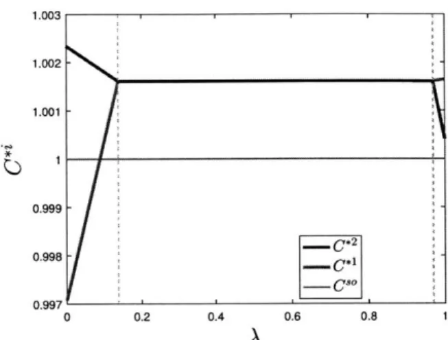
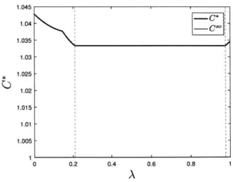
Next, we plot the expected population costs and the social cost in equilibrium. These costs are normalized by the socially optimum cost, denoted C, which is the minimum average social cost achievable by a fully informed social planner.

Symbol Value Units

,n 1 min/(veh- hr-1) 3 min/(veh- hr-1) C2 2 min/(veh- hr-1) b 20 min D 1 103veh/hr p 0.2 -f (n,t2) --fl* (a, t2)

I

1.003 1.0025 1 002 -1.001 -1.002 0.999 -1.0015 0.998 _* 0.997 - C 1 1.001-0.996 -C 0.995 1.0005 0.994-0 02 0.4 0.6 08 1 0 0.2 04 0.6 0.8 1 A A (a) (b)

Figure 2-2: Equilibrium population costs and equilibrium social cost

From this simple example, we analytically characterized the effect of the relative population sizes A on the equilibrium structure, population cost and social cost. In this article, we generalize these results to the environment in which two populations with asymmetric information about the network state but identical prefernces route their flows on a network.

Chapter 3

Model

Our modeling comprises of a network with an unknown state and state-dependent edge cost functions. Two information systems measure the network state with dif-ferent levels of accuracy and induce information heterogeneity among populations of travelers with identical preferences.

3.1

Environment

We model the transportation network as a directed graph g = (V, S) with a single origin-destination pair. Let V denote the set of vertices, and F the set of edges. Let R denote the set of routes connecting the origin and the destination. The network is in an environment with a random state s, which is drawn by a fictitious player "Nature" from a finite set S according to a prior distribution 0 E A(S). The cost function of any edge e

c

We introduce a set of two information systems, denoted I = {1, 2}. Each traveler

is exclusively subscribed to one information system. Travelers are modeled as a continuous player set with a fixed total demand D. We call the set of travelers

1Results in this article can be extended to the case with non-decreasing cost functions. For simplicity of our discussion, we focus on the case with increasing cost functions.

subscribed to the information system 1 (resp. information system 2) as population 1 (resp. population 2). Let us denote A as the population size parameter, and denote the fraction of population i's demand as A', where A' = A, A2 = 1 - A. Thus, the

demands of populations 1 and 2 are AD and (1 - A)D, respectively.

Each information system i

c

T

and |SI need not be equal. The joint distribution of the state s and the signals t1, t2 is denoted 7r

c

which satisfies the constraint that the marginal probability distribution on the state is equal to the prior distribution on state, i.e. for any s E S,

SZ

0(s). (3.1)

t1Efl t2ET2

The probability that population 1 and 2 receiving signals t' and t2

conditional on the state s E S, denoted p(t1, t2

Is), can be expressed as:

p(t1, t2 _{s) =}

_{7 (sti, ti),}

(tit

)

T.

0(s)

3.2

Bayesian Congestion Game

In the framework of Bayesian games (see Harsanyi (1967)), the notion of type captures the private information received by each population. In our model, the private infor-mation of population i is the signal t'. The type space of population i is T. Based on V, population i generates a belief about the state s and the other population's type t-, denoted pi(s, t-It) E A(S x Ti).

Each population routes its demand through the network based on its belief Pi (s, trjti). Population i's strategy is a map from the type (or signal) space V to a I7-dimensional vector, denoted q'(t') = (q'(ti))rE , where qg(t) is the demand assigned by popula-tion i to route r when its type is t. We say that a strategy profile q = (q', q2) is

feasible if it satisfies the following constraints:

q (t) = A D, Vt T , Vi I, (3.3a)

rE7Z

qz (tz) ;> 0, Vr E R, Vt" E T , Vi E I. (3.3b)

The constraint (3.3a) ensures that the demand of each population is routed, and the constraint (3.3b) imposes that demand assigned on each route is nonnegative. Let

Qi(A) denote the set of all feasible strategies of population i when the population size parameter is A. From (3.3a)-(3.3b), we note that the set of feasible strategy profiles, defined as Q(A) A Q1(A) x Q2(A), is a convex polytope.

We are now ready to define the Bayesian congestion game F. Formally,

A

F = (I, S, T, Q(A), C, p),

where:

I: Set of populations, I ={1, 2}

S: Finite set of states with prior distribution 0 E A(S)

7- = (Tl)iEx: Set of population type profiles (t1, t2

).

Q(A) = (Q (A))iEr: Set of feasible strategy profiles when the population size param-eter is A, with q = (ql, q2

) E Q(A)

C = {c- ()}eEE,sEs: Set of state-dependent edge cost functions

= (yp): M' is population i's belief about the state s and the other population's

type t-'

Importantly, our model assumes that the joint distribution ir is common knowl-edge. In addition to 7r, the set of network states S, the type sets jT| and IT21, the network graph (V, 8), the total demand D, the population parameter A, and the set of

ex ante interim ex post

Nature draws s Populations: -k'now their types Realize costs

Population i receives t _{-obtain beliefs pi(s, t-} Itz)

-play strategies

Figure 3-1: Timing of the game.

cost functions C are also common knowledge. The signal t' is the private information of population i.

The game is played as shown in Fig 3-1. In the ex ante stage, Nature draws a realization of the network state s E S according to the prior distribution O(s). Signals

(types) t1 and t2

are realized according to the conditional probability distribution

p(t', t2|s) in (3.2). In the interim stage, each population forms belief p (s, t-'It'), and

both populations choose their strategies q' simultaneously.

For any i E I and t E T, beliefs are obtained by Bayesian update on the common prior:

. r(s P, t-')

(s, t- It") = r(t,) Vs E S, Vt" E TZ

Pr(ti) (3.4)

where Pr(t) = EsEs t-iE- 7(s, tt)

For a given strategy profile q = (ql, q2

) C Q(A), the induced route flow is

f

, t2) is the aggregated demand assigned by populations with type profile (tl, t2

) on route r:

fr (t1, t2₎

= ql(t1) + q (t2_{), Vr E}

_R,

_C

Note that the dependence of

f

The induced edge load is w =

on edge e assigned by populations

We(t1, t2) = (ql(tl) + q ( 2))

r3e

q is implicit and is dropped for notational

conve-(We(t1, t2))eeS,(tt2)eT, where We(t1, t2) is the load

with type profile (t1, t2

):

3Ef(t, t2), Ve G E, V(t, t2) E T, (3.6)

r C R, denoted c,(q(t)) is:

c",(q(t)) =

3

eEsr

The expected cost of route r based on the interim belief p'(s, t-

It')

E[cr(q)|ti] = _{i(s,t-iti)CS(We(tit-i))} sES t-'eT-i e~r

-'ETi r s~c(we(ti,

t-2

)), Vr E R, Vt E t , V' C ,

sS8 t~e- Pr (ti) Ce

(3.8)

where We(t', t-') is given by (3.6).

We now define the equilibrium concept of the game F:

Definition 1. Bayesian Wardrop Equilibrium (BWE)

A strategy profile q* : T -+ Q(A) is a Bayesian Wardop Equilibrium (BWE) if for

any i c I, and any t' c T:

Vr E R, q*(t') > 0 -> E[cr(q*)t] < <E[ci(q*)|ti], Vr' C R. (3.9)

Equivalently, in a BWE, each population i with type t' assigns its demand only on the routes that have the smallest expected cost based on the interim belief P1(s, t-Iti).

We can define interim game2 IG(F) = (I, Q(A),

),

I = UieiT2: population set. Each type can be viewed as a population.

Q(A) Q ti (A)): strategy set. Each type t C T has strategy set Q (A) Q (A)

{

C -Er LEZrER

E [cr(q)

I t].

2_{Since the game has common prior, the ex ante game exists and is equivalent to the interim}

IG(IF) is a congestion game with type-specific cost function E[c,(q) ti]. It is shown in Milchtaich (1996) that generally there may not exist a potential function in a congestion game with player-specific cost functions. In our model, the type-specific cost function E[c,(q)jti] is based on ti's belief, which is obtained from the common prior 7r in (3.2). We show in Sec. 4.1 that due to the existence of common prior

r, the type-specific cost functions E[cr(q) t'] are related so that a weighted potential function exists in IG(F).

IG(P) is a complete information population game. A strategy profile ^* E Q(A) is

a Wardrop equilibrium of IG(), if for any r Ec7 R and any V G 1, q^*'(tP) > 0 implies

that

()

((q*'(t))t

(t2_))t

2 ) is a Wardrop equilibrium in IG(F). In rest of the article, we will refer to the Bayesian congestion game F and the interim game IG(F) interchangeably. We consider each type t' as a population. Consequently, a strategy of t' can be viewed as a IRI-dimensional vector qi(ti) =

(q'(ti)) , and a strategy profile can be viewed as a 7ZI x (IT1 + I T2) dimensional vector.

Chapter 4

Equilibrium Characterization

In this chapter, we study the equilibrium structure of the game F. In Sec. 4.1, we show that F is a weighted potential game, and that any equilibrium strategy profile is an optimum of a convex optimization problem. In Sec. 4.2, we study the qualitative properties of BWE when the population size parameter A varies from 0 to 1.

4.1

Weighted Potential Game

We adopt the definition of a weighted potential game with continuous player set from

Sandholm (2001):

Definition 2. Game F is a weighted potential game if there exists a continuously

differentiable function 4)(q) Q(A) -+ R and a set of positive, type-specific weights

{

O(<b(q (t))

= ^(t')E[c,(q)It'], Vr E R, Vt' E 'T, Vi E I.

Lemma 1. Game F is a weighted potential game with the weighted potential function

(J(q) as follows:

/ESe1

<(q) Y 7r

(s,

and the positive type-specific weight -y(t') = Pr(t') for any t' E T, i E I.

Proof. To show that 1(q) is a weighted potential function of F, we write the first order derivative of 1(q) with respect to qg(ti):

- E 7 r(s, ti, t2) c" (we(t , t-))

sES t- _eEr

( Pr(t)E[c(q)|t], Yr E R, Vt E T, Vi E I. (4.2)

We immediately obtain that 4)(q) satisfies Definition 2 with 7(t') = Pr(ti), Vti E T, Vi E I.

Note that (D(q) is a continuous and differentiable function of q. Following (3.5) and (3.6), 1 can be equivalently expressed as a function of the induced route flow

f

1D(f)

E

S

(s,t)

J3

sES eEC tET

(W)

Sr

sES eEC tET

For any feasible strategy profile q C Q(A), we note that 4b(q) 41(f) tD(w), where

f

Lemma 2. 4I(w) defined in (4.4) is continuously differentiable and strictly convex in

w.

Proof. Since each cs(we(t)) is differentiable in we(t), we conclude from (4.4) that D (w) is twice differentiable with respect to w. The first order partial derivative of 1(w) with respect to we(t) can be written as:

8We(t) = (s, t)c (w (t)) Ve C S, Vt E T,

and the second order derivative of <b(w) can be written as follows:

O

{we,('

t

Since for any e E ., s

C

(SIOdw,(t)

Thus, the Hessian matrix of 4(w) is a matrix with positive elements on the diagonal and 0 for all other entities, i.e. it is positive definite. Therefore, D(w) is strictly

convex in w. E

Theorem 1. A strategy profile q = (q', q2

) is a BWE if and only if it is an optimal

solution of the following convex optimization problem:

min <D(q) (OPT-Q)

s.t. q E Q(A),

where Q(A) is the set of feasible strategy profiles satisfying the constraints in (3.3).

We can write the Lagrangian of (OPT-Q) as follows:

(4.5)

L (q, p, v) = <t(q) + y Ae D -E (t)

iEI t'ET' rE-7 / rEIZ iEI tiC-ri

where p = (pjt)tEri,iE and v = (Vfl)rER,tiE-r,iEI are Lagrange multipliers associated

with the constraints (3.3a) and (3.3b), respectively.

Proof. We first show that a minimum of (OPT-Q) is a BWE. For any optimal solution

q, there must exist p and v such that (q, p, v) satisfies the following KKT conditions:

KKT DqI(t ) -DqV(t ) viq .(t2) = 0, ;> Vr CzR, Vt CT, ViEiC, Vr E R, Vt E r, Vi E i, Vr E R, Vt C, Vi E I. (4.6) (4.7) (4.8)

Using (4.2) and (4.6), we obtain that:

qi (ti) - Pr(t')E[c,(q)|ti] = p' + v, , Vr E R, Vti c T, Vi (E 21.

From (4.7), we see that for any r E R, any t' E T, and any i E I, if q (t') > 0,

the corresponding Lagrange multiplier vi = 0, and Pr(t)E[r(q)t] = pt. However, if q(t') = 0, Pr(ti)E[cr(q)jti] p' + vu ;> p". Thus, if q.(t') > 0 for a r E 7Z, ti

Tt, i E I, then:

Pr(t)E[c,(q)jt_{'] = pt < Pt + vt'l}

= Pr(t)E[r'(q)It'], Vr' E R,

which implies that E[cr (q) It] < E [cr (q) It'] for any r' E ). Recalling Definition 1, we conclude that q is a BWE if it is an optimal solution of (OPT-Q).

Next, we show that any BWE q* is an optimal solution of (OPT-Q). We define a pair of Lagrange multipliers (p, P), where f!t = minrcE Pr(t)E[cr(q*)It'], and ri =

Pr(t)E[r(q*)Iti] - ft. We can easily check that (4.6) and (4.8) are satisfied by

such (q*, p, ). Since q* is a BWE, from Definition 1, if q*(ti) > 0, E[cr(q*)|ti] = minre JE[c,(q*)jtf]. Thus:

F = Pr(t)E[cr(q*)|ti] - fzti = Pr(tt) E[cr(q*)Iti] - minE[cr(q*)It] 0.

,ER

Consequently, (4.7) is also satisfied by (q*, p, P). Recall (D(q) = <D(w), since w is an affine function of q (see (3.6)) and 4D(w) is strictly convex in w (Lemma 2), 'D(q) is a convex function of q. Additionally, Q(A) is a convex polytope, (OPT-Q) is a convex problem. Thus, KKT conditions are sufficient for optimality, and q* is an optimal

solution of (OPT-Q). l

The existence of BWE follows directly from Theorem 1. We denote the set of equilibrium strategy profiles as Q*(A). For any BWE q* E Q*(A), we define sets

M(q*) and N(q*) as the set of p* and v* such that (q*, P *, v*) satisfies the KKT

Next, we show that the equilibrium edge load w* induced by any q* E Q*(A) is identical.

Corollary 1. The BWE edge load w* is unique.

Proof. For any q* E Q*(A), <b(q*) = 4b(w*) is identical. Since D(w) is strictly convex

in w (Lemma 2), we conclude that w* is unique. 0

Proposition 1. For any q* E Q*(A), M(q*) and N(q*) are singleton sets with

ele-ments of I*, v*:

*= min Pr(ti)E[cr(q*)jti], Vti E T, Vi E 1. (4.9) vl"* =Pr(t')E[C,(q*)lt4] - [i*, Vr

Cz

I.

Furthermore, both p* and

v*

Proof. First, we argure by contradiction that Linear Independence Constraint Qual-ifications (LICQ) defined in definition 3 in Appendix A is satisfied in (OPT-Q). We denote the set of constraints that are tight at optimum in (3.3b) as B A {qr*(ti) q*i(ti) = 0, Vr E R, Vti

c

c

in (3.3a); hence we arrive at a contradiction.

We know from Proposition 10 in Appendix A that if LICQ holds, for any q* E

M(q*) and N(q*) are singleton. From the proof of Theorem 1, we know that for any q* E Q*(A), (q*, A*, v*) satisfies the KKT condition, where p*, v* are defined in (4.9)

and (4.10). Furthermore, the equilibrium edge load induced by any q* G Q*(A) is identical (Corollary 1). From (3.8), p* and v* are identical for any q* E Q*(A). El

Proposition 1 connects the smallest expected route cost for each type t' at equi-librium with the unique Lagrange multiplier p"*. This result will be used again when we discuss the relative value of information in Chapter. 5.

Theorem 1 shows that the equilibrium strategy profile can be solved as the solution of a convex optimization problem (OPT-Q). However, characterizing q* as A varies directly from (OPT-Q) is difficult. On one hand, feasible set (and hence the optimal set) of (OPT-Q) changes with A; see (3.3a)-(3.3b). On the other hand, we observe from two route example in Chapter 2 that the induced route flow may be identical for a certain range of A. We approach the question of characterizing Q*(A) by studying

how the set of equilibrium route flows change with A. We proceed in two steps: First, we represent the set of feasible route flows as a polytope. For any feasible route flow, we characterize the set of feasible strategy profiles that can induce it in Proposition 2. Next, we study how the equilibrium route flows change with A via an auxiliary optimization problem (Proposition 3)

We define F(A){f E RIIX ITI If satisfies (4.11)

},

fr(t 1, t2) + fr (, F2) = fr(ti, ) + fr(f, t2), Vr E R, Vt1 , EE T1, and Vt2_,2 E -2 (4.11a) fr (tl, t2) = D, V (t1, t2

)

fr

,

E R7,

(tI,

)

E

T,

min

<

C

T.

Proposition 2. The set of feasible route flows is F(A) defined in (4.11). F(A) is a

convex polytope.

that induces

f

q = f(t1, 2) - f 2(t") Xr7, Vr E r, Vt E T, (4.12a) q (t2) = fr(P, t2

) Xr, Vr E R, Vt2

C

where () is any type profile in T, and (Xr)r7Z is any

|R|-dimensional

,

AD,

Proof. First, we show that any route flow

f

satisfies (4.11). Following (3.5), we obtain:

fr(t1, t2) + fr(il, 2) =ql4t1) + q (t2) + q (11)+ q2tj)

=fr(tl, t2) + fr(t, t2), Vr

E

T2,

which implies that f satisfies (4.11a). From (3.3a) and (3.3b),

f

C T2

D

-

tE EtIET 1 tOET

rE7Z rEIZ rE1Z rElZ

Therefore,

f

f

f

Next, we show that for any

f

q

E

consider any x satisfies (4.13):

X AD > D - min f(tt2)=5 max (f(f, ) - f(t1, P)).

rElZ e b E T rEiZleT ,

(4.11a), we have:

fr(f, t2) + fr(tI, 2) - fr(p, 2) (3)q(t1I) + 2(t2) (3gb) 0, fr (f, t2) fr(p, 2) fr(t , 2),

min f (t I, t2 2 max

(f,(fl,

t2ET2 t1E71

Thus, the set of x satisfying (4.13) is non-empty.

f, (t1, 2)) ,

For any

Q

=

S

E

C

Similarly, we can show that 42 also satisfies (3.3a) and (3.3b). Thus, 4 is feasible. To check that 4 induces the route flow

f:

qI(tI) + 2 (t2) = fr(t1, 2) - fr(',t 2) + fr(Pt2

) (4

f(t',

), Vr E R, t E T , t2 C T2_.

Therefore, for any f satisfies constraints (4.11), there exists feasible strategy profiles that can induce

f.

Actually, (4.11d) and (4.11e) are equivalent to the following affine constraints:

Vtlr C

7-,

A,

E T

t2 T2.

2,t E

T'.

Thus, F is a convex polytope.

Finally, we show that for any feasible route flow

f

Vr E R, t I E

Tt

Vr

R7,t

Tt

VP

C

T,

< A,

)

-strategy that can induce f is in (4.12). For any route r E R, the system of equations in

(3.5) contains

IT I

IT

IT'I+IT

For any given F E VT, P E T2_,

the following equations are linearly independent:

l'(t) + q 2

(2 ) = fr(t, j2), Vt C T1.

r r _(4.16)

q'(P)+ q (t2_{) = fr(P, t}2_{), Vt}2 _{E T2 \ {j2}.}

Any constraint for that r in (3.5) can be derived from (4.16):

qr(t') +q|(t 2 ) = (ql(P) + q (2)) + (q(f) + q(t2 )) - (ql(t1) ++ t2(t 2 )) (416) f (t' f) + fr( 1, t2) - 2 fr(ff2) (4.1a)

f

E

T

.

Thus, for any r, (3.5) contains

IT1

I+

_I

variables. From the rank-nullity theorem, the dimension of its null space is 1. Any solution of (3.5) can be expressed as (4.12), where P E TE, P E T2 are any given type of population 1 and 2, and X, E R is a free variable.

From (4.14) and (4.15), to ensure that q is a feasible strategy profile, (Kr)r must satisfy (4.13). We know from previous discussion that when f C F(A), such X exists. Consequently, the set of feasible strategies that can induce

f

Any given (P, P) E T determines a set of basis in (3.5). The set of feasible strategies represented by (4.12) is identical for any chosen (f, P). l

The constraints (4.11) can be understood as follows: (4.11a) captures that aggre-gated flows assigned by the same set of types are equal. (4.11b) ensures that all the demand D is routed, and (4.11c) guarantees that the demand assigned to any route

is nonnegative. (4.11a), (4.11b) and (4.11c) are unrelated to A.

Next, we interpret (4.11d)-(4.11e). For any q E Q(A), we define J4(q) as follows:

Z)

(q.(a)-J~~~(q)ma (

where V is any type in 'P.

Ji(q) is the summation over all r of the maximum difference in the demand

assigned to route r by type 0 comparing to any type P E Ti.

Jf(q)

Ji(q) can be rewritten in terms of the induced flow

f:

(f) - '(q) = max(fr(i, i-') - fr(tih-)),

rE1Z

= D - i fr(ti, f~i)) (4.17)

where (P, i) is any type profile in T. Thus, constraints (4.11d) and (4.11e) can be restated as:

1

(f) < AD, (4. 11d')

j2(f) (1 - A)D. (4.11e')

Constraints (4.11d') and (4.11e') ensure that the impact of signals on each popula-tion's strategy (Ji(f)) is bounded by its demand.

We note two cases: On one hand, if gq(ti) is identical for all t'

E

received by population i does not effect population i's strategy, then Jf(f) is 0. On the other hand, note that for any i E I:

Ji(q) = A'D min q (ti) = 0, Vr E R. (4.19)

The second case plays a key role in distinguishing equilibrium regimes in Sec. 4.2. We next present the auxiliary optimization problem for solving equilibrium route

flows.

f

min 4(f) _(OPT-T)

s.t. f E T(A),

where 1b(f) is given by (4.3), and F(A) is the set of feasible route flow vectors defined

by (4.11).

Proof. We first show that in any BWE, the route flow f* is an optimal solution of (OPT-F). By definition,

f*

minfey $(f), then there exists a feasible route flow f E F(A), which is induced by a feasible strategy q c Q(A), such that D(q) = (f) < (f*) = D(q*). This is a

contradiction, because by Theorem 1, q* must minimize 4(q). Thus,

f*

Next, we show that any optimal solution of (OPT-F) say f* is an equilibrium route flow. Since

f*

Now assume that q is not a BWE, then there exists an equilibrium q*' C Q(A) and an

induced flow

f*'

the fact that

f*

To sum up,

f

f

Proposition 3 forms the basis of our further investigation. Note that among the constraints (4.11) which define the set of feasible route flows,

f

and (4.11e) depend on the relative populationm size A. We show in section 4.2 that the tightness of these constraints leads to the qualitatively different equilibrium regimes (Theorem 2).

4.2

Equilibrium Regimes

In this section, we study how BWE changes when the relative population size A changes. Let ft denote an optimal solution of a simpler optimization problem:

min

$(f)

s.t. (4.11a), (4.11b) and (4.11c)

That is ft minimizes potential function 4)(f) and satisfies the constraints that are independent of A. Following the same analysis in Corollary 1, since (1(w) is strictly convex in w, any ft induces identical edge load wt. The optimal solution set, denoted

yt, can be written as:

{

f

(t)

(t),

T

Recall the two-route example in Chapter 2, there is a range of A such that the equilib-rium route flow does not change with A. We will show next that we can find a range of A such that the equilibrium edge load does not change with A, and w*(A) = wt.

From (4.20), TF is a bounded polytope. We define A and A as follows:

A min {J'(f') , (4.21)

D fteyt

max _2(ft). (4.22)

D ftErt I

Since yt is a bounded polytope, and J(ft) is continuous in

ft,