Dynamical System Modeling of a Micro Gas Turbine Engine
by
Chunmei Liu
B.S., Harbin Institute of Technology (1988)
M.S., Harbin Institute of Technology (1991)
Submitted to the Department of Aeronautics and Astronautics
in partial fulfillment of the requirements for the degree of
Master of Science
at the
MASSACHUSETTS INSTITUTE OF TECHNOLOGY
June 2000
@
Massachusetts Institute of Technology 2000. All rights reserved.
Author
...
Department of Aeronautics and Astronautics
May 12, 2000
C ertified by ...
...
. . .
...
. .
James D. Paduano
rincipal Research Engineer
Thesis Supervisor
/1
Accepted by ...
Nesbitt W. Hagood, IV
Professor of Aeronautics and Astronautics
Chair, Committee on Graduate Students
MASSACHUSETTS INSTITUTE
OF TECHNOLOGY
SEP
0 7 2000
Dynamical System Modeling of a Micro Gas Turbine Engine
by
Chunmei Liu
Submitted to the Department of Aeronautics and Astronautics on May 12, 2000, in partial fulfillment of the
requirements for the degree of Master of Science
Abstract
Since 1995, MIT has been developing the technology for a micro gas turbine engine capable of producing tens of watts of power in a package less than one cubic centimeter in volume. The demo engine developed for this research has low and diabtic component performance and severe heat transfer from the turbine side to the compressor side. The goals of this thesis are developing a dynamical model and providing a simulation platform for predicting the microengine performance and control design, as well as giving an estimate of the microengine behavior under current design. The thesis first analyzes and models the dynamical components of the microengine. Then a nonlinear model, a linearized model, and corresponding simulators are derived, which are valid for estimating both the steady state and transient behavior. Simulations are also performed to estimate the microengine performance, which include steady states, linear properties, transient behavior, and sensor options. A parameter study and investigation of the startup process are also performed.
Analysis and simulations show that there is the possibility of increasing turbine inlet temper-ature with decreasing fuel flow rate in some regions. Because of the severe heat transfer and this turbine inlet temperature trend, the microengine system behaves like a second-order system with low damping and poor linear properties. This increases the possibility of surge, over-temperature and over-speed. This also implies a potentially complex control system. The surge margin at the design point is large, but accelerating directly from minimum speed to 100% speed still causes surge. Investigation of the sensor options shows that temperature sensors have relatively fast response time but give multiple estimates of the engine state. Pressure sensors have relatively slow response time but they change monotonically with the engine state. So the future choice of sensors may be some combinations of the two. For the purpose of feedback control, the system is observable from speed, temperature, or pressure measurements.
Parameter studies show that the engine performance doesn't change significantly with changes in either nozzle area or the coefficient relating heat flux to compressor efficiency. It does depend strongly on the coefficient relating heat flux to compressor pressure ratio. The value of the compressor peak efficiency affects the engine operation only when it is inside the range of the engine operation. Finally, parameter studies indicate that, to obtain improved transient behavior with less possibility of surge, over-temperature and over-speed, and to simplify the system analysis and design as well as the design and implementation of control laws, it is desirable to reduce the ratio of rotor mechanical inertia to thermal inertia, e.g. by slowing the thermal dynamics. This can in some cases decouple the dynamics of rotor acceleration and heat transfer.
Several methods were shown to improve the startup process: higher start speed, higher start spool temperature, and higher start fuel flow input. Simulations also show that the efficiency gradient affects the transient behavior of the engine significantly, thereby effecting the startup process.
Finally, the analysis and modeling methodologies presented in this thesis can be applied to other engines with severe heat transfer. The estimates of the engine performance can serve as a reference of similar engines as well.
Thesis Supervisor: James D. Paduano Title: Principal Research Engineer
Acknowledgements
I would like to express my gratitude to Dr. Paduano for his invaluable guidance and direction
throughout the course of this research, as well as his continuous encouragement and support. I would also like to thank John Protz, who discussed nearly every piece of my research with me and gave precious suggestions; Yifang Gong, who was always there when I was stuck in the research. I would also like to give my special thanks to Prof. Epstein and Dr. Tan who made my research possible and gave me their guidance. In addition, I would like to acknowledge Dr. Stuart Jacobson for his help and willingness to answer all my questions.
I am also grateful to all those people who have helped me to make my stay here a pleasant one.
In particular, I'll like to thank Yang-Sheng Tzeng and Shengfang Liao, as well as my officemates Kenneth Gordon, Brian Schuler, Sanith Wijesinghe, and Margarita Brito, who helped me a lot on my research, classes and the daily life; Lori Martinez, for her cheerfulness and friendliness; all other people in the microengine project and GTL, for the data, help and cooperations. I'm also thankful to many of my friends both here in the USA and there in China, who continue to give me a colorful life and are ready to give me a hand whenever I need one.
Last but not least, I'd like to thank my husband, my parents and my sisters, who are forever my sources of inspiration, encouragement, and support.
Contents
1 Introduction
1.1 B ackground . . . . 1.2 Technical Objectives and Development Approaches . . . .
1.3 Contributions and Organization of the Thesis . . . .
2 Microengine Modeling and Simulator Development
2.1 Order of Magnitude Analysis . . . . 2.1.1 Rotor Acceleration Dynamics . . . . 2.1.2 Gas Dynam ics . . . .
2.1.3 Heat Transfer Dynamics . . . . 2.1.4 Dynamics of Emptying the Fuel Tank . . . .
2.1.5 Summary of the Order-of-Magnitude Analysis of the Dynamics . 2.2 Nonlinear Model and its Simulator . . . . 2.2.1 Component Characteristics . . . . 2.2.2 Modeling of the Dynamics . . . .
2.2.3 Nonlinear Model Simulator . . . .
2.3 Linearized Model and its Simulator . . . . 2.3.1 General Aspects of the Linearized Models . . . .
2.3.2 Linearized Model and Simulator for the Microengine . . . . 2.4 Sum m ary . . . .
3 Simulation Results
3.1 Simulation Objects . . . . 3.2 Minimum Achievable Speed and Steady States - T4 1 Behavior with mif .
3.2.1 3.2.2 3.3 Linear
3.3.1
Mathematical and Physical Explanations of the T4 1 Behavior with nif . . . .
Simulation Verification of the T4 1 Behavior with mf. . . . .
P roperties . . . . Simulation Descriptions . . . . 15 . . . . 15 . . . . 16 . . . . 17 21 . . . . 21 . . . . 21 . . . . 22 . . . . 23 . . . . 25 . . . . 26 . . . . 27 . . . . 27 . . . . 31 . . . . 39 . . . . 41 . . . . 41 . . . . 41 . . . . 43 51 51 52 52 53 54 54
3.3.2 Simulation Results and Analysis . . . . 55
3.4 Transient Properties . . . . 56
3.4.1 Time Domain Step Response . . . . 56
3.4.2 Damping and Natural Frequency . . . . 57
3.4.3 Acceleration from Minimum Speed to 100% Speed . . . . 57
3.5 Sensor O ptions . . . . 58
3.6 Sum m ary . . . . 59
4 Parameter Studies and Startup Process 81 4.1 Param eter Studies . . . . 81
4.1.1 Parameter Descriptions and Behaviors Studied . . . . 81
4.1.2 Simulation Results for Parameter Studies . . . . 83
4.2 Startup Process . . . . 85
4.2.1 Startup Procedure . . . . 85
4.2.2 Startup Process on Diabatic Experimental Compressor Map . . . . 86
4.2.3 Startup Process on Modified Diabatic Experimental Compressor Map . . . . 86
5 Conclusions and Future Work 107 5.1 Conclusions . . . . 107
5.2 Recommendations of Future Work . . . 109
List of Figures
1-1 The MIT Demo Microengine ...
1-2 Demo Microengine Mechanical Layout ...
Helmotz Resonator Model for the Microengine . . . .
Hypothetical Compressor Map . . . . Adiabatic Experimental Compressor Map . . . . Diabatic Experimental Compressor Map - 3D . . . .
Diabatic Experimental Compressor Map - 2D Representation . .
Modified Diabatic Experimental Compressor Map with Heat Flux eter Study... ...
Turbine M ap . . . . Engine Cycle Model Structure . . . . Simulation Signal Flow Diagram . . . .
. . . . 45
. . . . 45
. . . . 46
. . . . 46
. . . . 47
- Used for Param-. Param-. Param-. Param-. Param-. Param-. Param-. Param-. Param-. Param-. Param-. 47
. . . . 48
. . . . 49
. . . . 50 3-1 Running Line of Nonlinear Model . . . .
3-2 Steady States of Nonlinear Model . . . .
Steady States vs Fuel Flow for Different Shaft-off-take Power and Turbine Map . . .
Steady States Comparisons between Linearized Model and Nonlinear Model . . . . . Time Domain Transients Comparisons between Linearized Model and Nonlinear Model Transients Comparisons on Compressor Map between Linearized Model and Nonlinear Model .. ... ...
Root Distribution - Object 3 . . . . Typical Time Domain Step Response of Nonlinear Model . . . . Characteristics of Second-order Systems . . . . Acceleration from Minimum Speed to 100% Speed . . . . Thrust Change with T3, T41, T45 and P3, P41, P45 . . . .
Running Line - Parameter Study . . . . Steady States - Parameter Study . . . .
61 63 64 66 70 71 72 74 75 77 79 91 97 19 20 2-1 2-2 2-3 2-4 2-5 2-6 2-7 2-8 2-9 3-3 3-4 3-5 3-6 3-7 3-8 3-9 3-10 3-11 4-1 4-2
4-3 Root Distribution - Parameter Study . . . 100
4-4 Startup Process on Compressor Map - Diabatic Experimental Compressor Map . . . 101
4-5 Time Domain Startup Process - Diabatic Experimental Compressor Map . . . . 101
4-6 Startup Process on Compressor Map -Set Minimum Efficiency, on Modified Diabatic Experimental Compressor Map . . . . 102 4-7 Time Domain Startup Process - Set Minimum Efficiency, on Modified Diabatic
Ex-perimental Compressor Map . . . . 103
4-8 Startup Process on Compressor Map - Change Efficiency Gradient, on Modified Dia-batic Experimental Compressor Map . . . . 104 4-9 Time Domain Startup Process - Change Efficiency Gradient, on Modified Diabatic
List of Tables
2.1 Default Line Types for Lines with Heat Flux and without Heat Flux . . . . 29
3.1 Data Analysis for T4 1 Trends with my . . . . 53 3.2 Default Line Types for Nonlinear Model and Linearized Model . . . . 55 3.3 Comparisons of Acceleration Time Constants between Microengine and T700 . . . . 57
4.1 Notation of Graphs for Parameter Study . . . . 83
4.2 Summary of Results from Parameter Study . . . . 85
Nomenclature
Roman
a Speed of sound; constant
A Area; coefficient matrix
B Coefficient matrix
C Coefficient matrix
C, Specific heat at constant pressure
D Coefficient matrix
e Constant
f
Fuel-to-air ratio; functionh Heat value of the fuel; convective heat transfer coefficient
J Rotor inertia
k Constant
L Length
m Mass
M Mass; Mach number
N Rotation speed
P Total pressure
Power Power
R Gas constant; radius
Re Renolds number T Total temperature u Speed V Volume Work Work z Constant
Greek
3 Angley Ratio of specific heats
r1 Efficiency
7r Total-to-total pressure ratio
r Time constant; characteristic time; temperature ratio
p Density
Superscripts
abs Absolute value
no Value with no heat flux
rel Relative value
Subscripts
0 Operating point 2 Inlet of the compressor
3 Exit of the compressor 41 Inlet of the turbine 45 Exit of the turbine
acc Acceleration
b Combustor
c Compressor
cm Thermal inertia
comp Compressor
des Design point
ef Efficiency
f
Fuelgas Gas dynamics
jg
Mechanical inertiamin Minimum value
n Nozzle
p Percentage pi Pressure ratio
q Heat flux related
rad Radial component
s Static quantity
t Turbine; total quantity; temperature related
tan Tangential component
thermo heat transfer dynamics
turb Turbine
v Volume related
w Spool
Full quantities
C. Specific heat of the rotor
epeak Peak efficiency the compressor can reach
m Mass flow rate
P Static pressure
Q
Heat fluxChapter 1
Introduction
1.1
Background
Recent advances in the field of fabrication have opened the possibility of building a micro-gas turbine engine. MIT is developing the technology for such engines. These are millimeter to centimeter-size heat engines fabricated with semiconductor industry micromachining techniques. As such, they are micro electro-mechanical systems (MEMS) devices. They contain all the main functional components of a conventional large-scale gas turbine engine. Preliminary studies show that these devices may ultimately be capable of producing 10-100W of power or 10-50 grams of thrust in less than a cubic centimeter. Applications include battery replacements, propulsion for small air vehicles, and a variety of blowers, compressors, and heat pumps.
Refractory structural ceramics, such as silicon nitride (Si3N4) and silicon carbide (SiC), have
excellent mechanical, thermal, and chemical properties for gas turbine applications permitting un-cooled operation up to the 1500-1700K combustor exit temperature range ([1]). While there is an ongoing effort to develop the needed SiC microfabrication technology, sufficient technology has not been demonstrated to date. On the other hand, most of the necessary technology has been demon-strated in silicon. Thus, for simplicity of construction and minimum technical risk as opposed to high power output and good fuel consumption, current efforts are focused on demonstrating a work-ing micro gas turbine engine, the "demo-engine", which is made of silicon. Based on the analysis and design experience obtained from this demo engine, as well as the process development for more refractory materials, the final high temperature microengine will be built.
The baseline design of the demo engine (henceforth referred to as the "microengine") is shown in Fig. 1-1. Its basic geometry and parameters at the design point can be found in Fig. 1-2 ([9]). It has several characteristics which are different from conventional large-scale engines, some of which are listed below:
. Small scale.
" Low and diabatic component performance.
The micro compressor and the micro turbine are a few millimeters in size. Hence, even at transonic tip Mach numbers, the Reynolds number is of the order of a few thousands only. This low Reynolds number, as well as the micofabrication constraints, lead to low component performance ([8]). In addition, the component performance is a function of the heat flux, as shown below.
" Heat transfer.
Because of the low component performance, a combustor exit temperature greater than 1400K is needed for self-sustaining engine operation. But silicon must remain below about 950K to retain sufficient strength for the rotating structure ([1]). The approach of rejecting the heat the turbine absorbs into the compressor flow path was chosen to cool the turbine. This heat transfer from the turbine side to the compressor side has two negative effects. One effect is that the heat transfer dynamics become strongly coupled with the rotor acceleration dynamics (this effect will be discussed in detail in the following chapters). Another effect is the reduction of the component performance ([1]). Although the effect on turbine performance is relatively small, the effect on compressor pressure ratio and efficiency is significant.
Since these characteristics seldom exist in conventional large scale engines, they motivate us to investigate the performance and dynamic behavior of an engine with these characteristics. From the microengine project perspective, the results will enable prediction of the microengine performance. From a general perspective, the results can serve as a reference for future design and analysis of similar engines.
1.2
Technical Objectives and Development Approaches
The overall objectives of the thesis are to derive a model for the microengine which can describe the micriengine behaviors and to provide a simulation platform to estimate engine behavior. These objectives are pursued by performing the following steps:
* First the dynamics of the main engine processes are investigated and the important ones are determined.
" Then, component performance information is assembled based on the current available data. " Based on the dynamics analysis and the component performance, a nonlinear model for the
microengine is derived. This model is valid at both design and off-design points, and can describe transients as well.
" Linearized models are derived by linearization around steady operating points. These linearized models enable us to make use of the large body of results for linear systems to analyze the properties of the system, especially the transient properties. The linearized models will also be references for the development of control systems in the future.
" The simulators corresponding to the nonlinear model and linearized models are developed
using a combination of C code and the Matlab/Simulink interface for dynamics and control.
Another objective of this thesis is to estimate the engine performance using the developed sim-ulators. The performance characteristics that are of interest include:
" the running line and the steady states;
* the linear properties;
" the stability and the transient acceleration and deceleration processes; " sensor options for measuring system behavior and for feedback control;
" the effect of the reduction of the compressor pressure ratio and efficiency to the engine
perfor-mance, due to the heat addition into the compressor;
" the effect of the limit peak efficiency which the compressor can reach;
e the effect of the heat transfer dynamics; " the effect of the nozzle area;
e the startup process.
1.3
Contributions and Organization of the Thesis
The main contributions of the thesis are:
1. obtaining the models for the engine with heat transfer;
2. providing a simulation platform for the overall engine behavior and future work;
3. finding out the main characteristics of the microengine performance, which include:
* Due to the heat transfer dynamics, the system becomes a second-order system instead of a first-order system, which is one of the main differences from a conventional engine. The spool behaves like an energy storage device.
" There is the possibility of increasing T4 1 with decreasing nfi in some regions, which is
" The system behaves quite different at different operating points, and the linear properties are not good.
" The acceleration time constant is on the order of several hundred milliseconds.
" The lowest damping of the second-order system can reach 0.15, and the corresponding
overshoot can be as large as 62%. Thus under some conditions it is possible to get over-temperature or over-speed unless precautions are taken.
" The surge margin is relatively large, but accelerating the engine from minimum speed
to 100% speed will still cause surge. Therefore, an engine of this type would have to incorporate a control system to avoid fast acceleration.
4. investigating the sensor options. There are two aspects regarding the sensor choices. One aspect is for measuring the current engine operating point. Another aspect is for providing feedbacks for the future control system. Both are considered in this thesis.
5. performing sensitivity analysis of the engine performance to certain elements. The elements
include: the reduction of the compressor performance due to the heat addition, the limit peak efficiency the compressor can reach, the heat transfer dynamics, and the nozzle area.
6. simulating several procedures for the startup process, which include: start the engine at
dif-ferent speeds, difdif-ferent fuel inputs, and difdif-ferent spool temperatures. The effect of efficiency gradient of the compressor map on the startup process is simulated as well.
The organization of the thesis is as follows: chapter two analyzes the main dynamical elements in the microengine system, assembles the component characteristics, and derives the nonlinear and lin-earized models, as well as their corresponding simulators. Chapter three gives the simulation results for the microengine, which includes the steady states and transient behaviors of the microengine, the special properties of the microengine performance compared with conventional engines, and the
sensor considerations. Chapter four investigates the effects of several elements on the engine perfor-mance, which include: the reduction of the compressor performance due to heat addition, the limit peak efficiency the compressor can reach, the heat transfer dynamics, and the nozzle area. These investigations are referred to as "parameter studies". Chapter four also investigates the startup process. Chapter five draws conclusions for the overall work done and gives some recommendations for future work.
Starting
Air In
Compressor Inlet
Exhaust
Turbine
Combustor
21 mm.
11g
Thrust
16g/hr
H2 Fuel Burn
1600K (2420 F) Gas Temp.
1.2 million RPM rotor
3D Schematic Diagram
GeometrY
-Die
Size
= 2.1 cm
-Comb.
Vol
= 195mm
3-
Bearing Depth = 500 um
-
Comp. Radius = 4 mm
-
Turb. Radius = 3mm
Bearings
-
Speed
-
/D
-
Clear
-
Rad.
-
Run Gap:
=1.2M RPM
=.1
=15-20 um
=3
mm
=1-2 um
ZVCompressor
-
OPR
-
mdot
-
Tip Speed = 5
-
Heat Flux
=4C
1.8
0.36 g/sec
00
M/sec
-50
W
Turbine
-
Power
-
Stress
-
Tt gas (rel)
-
T struct
-
Heat Flux
=50
W
~
500 Mpa
~
1450 K
=950 K
40-50 W
Combustor
-
Tt4
= 1600K
- T
struct
=1200K
-
Res. Time
=0.1
ms
Chapter 2
Microengine Modeling and
Simulator Development
This chapter derives dynamical models for the microengine, including both a nonlinear model and linearized models, as well as corresponding simulators. First the dynamics of the primary physical processes in the miroengine are investigated in order to determine which processes are important and should be incorporated in the model; then the nonlinear model and its corresponding simulators are developed; finally the linearized models are derived by linearization around the steady points.
2.1
Order of Magnitude Analysis
There are three main dynamical elements that are accounted for in this analysis: rotor acceleration, gas dynamics, and heat transfer. In addition, there is another dynamical element which may be important during the operation of the microengine: the dynamics of emptying of the fuel tank. This section estimates the time constants of these processes and determines the important dynamics, in order to arrive at a simple and effective model.
2.1.1
Rotor Acceleration Dynamics
The time constant for the rotor acceleration dynamics can be estimated using [7]:
47r2 JN 2 Y
Tace =CeT
2 m2 (Tc)o'
where the subscript "0" refers to the current operating point, racc is the approximate acceleration
time constant, J is the rotor inertia, N is the rotation speed in rps (i.e., the units for 27rN are
compressor, T2 is the total temperature at the inlet of the compressor, m2 is the air mass flow at
the inlet of the compressor, and -r is the temperature ratio of the compressor.
The parameters for the microengine at its design point, as well as the other parameter needed are (Fig. 1-2 and [9]):
27rN 1.2 x 10⁶rpm ~ 1.25 x 10⁵rad/s, y = 1.4, J = 9.3 x 10- 10 kgm2 , C = 1004.5J/kgK, T2 = 300K, M2= 0.36g/s = 0.36 x 10⁻³kg/s, (rc)o ~ 1.38.
Using these values, the time constant of the rotor acceleration can be estimated as:
racc ~ 0.34s. (2.1)
2.1.2
Gas Dynamics
The engine is modeled as a Helmoltz resonator ([5]) to analyze the gas dynamics, as shown in Fig. 2-1. By applying mass conservation, momentum conservation, and assuming:
U2 U3 U, P3 = P4 1 P,
APr= rkTrUl.
2
where the subscripts "2", "3", "41" and "45" refer to the inlet and exit of the compressor and the turbine, respectively, as shown in Fig. 2-1. u is the air speed, P is the pressure, APT P4 1 - P45
is the pressure drop across the turbine, and kT is a constant.
The characteristic time of the gas dynamics can be computed ([5]) to be:
1 LeVb
Tgas dyam
Vb i
characteristic length of the duct of the compressor, ab is the speed of sound in the combustor, and
Ab is the average area of A3 and A4 1.
For microengine, according to Fig. 1-1, Fig. 1-2 and [9], the geometry is as:
Le ~ 13mm,
Ab e 3.87rmm2,
Vb ; 190mms
Using these values, an estimate for the gas dynamics characteristic time is:
Tgas 0.05s, (2.2)
which is much smaller than the rotor acceleration time constant.
2.1.3 Heat Transfer Dynamics
This subsection estimates the heat transfer dynamics. Due to the relatively high thermal conduc-tivity of silicon, the microengine has large heat flow from the turbine side to the compressor side (40W compared to the 40W of shaft power absorbed by the compressor) [10]. This heat flow not only decreases the compressor pressure ratio and efficiency and lowers the thermodynamic efficiency of the cycle, but also makes the dynamics of the engine more complex. This is because its dynamics lie in the same range as the rotor acceleration, which will be shown by estimating the time constant of the heat transfer dynamics.
In the heat flux path, the major sources and sinks are the fluid across the compressor and the turbine. Other minor sources and sinks include the blade tips, the seals and the journal bearing
([10]). Here for the first order estimation, these minor heat sources and sinks are neglected, and the
following assumptions are made:
" uniform temperature of the whole spool T,;
" bulk temperature and bulk heat transfer coefficients can be used;
" the bulk heat transfer coefficients are independent of the flow and the structural temperature;
* when calculating the heat flux from the flow at the turbine side into the rotor and the heat flux from the rotor into the flow at the compressor side, we can use characteristic bulk temperatures
Tturb and Tcomp to approximate the temperature of the flow on the turbine side and the compressor side, respectively.
Based on these assumptions, the heat flux from the flow at the turbine side to the rotor Q and the heat flux from the rotor to the flow at the compressor side Q can be represented as:
Qt= htAt(Turb - Tw),
QC= heAc(Tw - Tcomp),
where At and Ac are the convection area at the turbine side and the compressor side, respectively, and ht and he are the convective heat transfer coefficients at the turbine side and the compressor side, respectively.
Thus, the net heat flux flowing into the rotor is:
Q=Qt -
Qc=
htAt(Tturb - Tw) - heAc(T - Tcomp) hA(T - Tw), (2.3)where
hA = htAt + heA,
and
T = htAtTturb + hcAcTcomp ht At + he Ac
Applying energy conservation for the spool yields the following:
dTw
Q= CWM dt (2.4)
where Cw and M, are the specific heat and the mass of the rotor, respectively. Combining equa-tion 2.3 and equaequa-tion 2.4, we arrive at:
dTw
CWMW y dt = hA(T - Tw).
Therefore the time constant for the thermal dynamics is approximately:
Tthermo
-For the microengine, the data is as follows [4, 9):
Cw ~ 700J/kgK (silicon property at T ~ 1600K), pw ~ 2400kg/rm, Vw ~ 10 8n3 (1Omm3), h ~ 1000w/m 2 K,
A ~ 10- 5 - 104m2.
Using these values the thermal time constant can be estimated as follows:
7thermo ~ 0.17 - 1.68s. (2.6)
2.1.4
Dynamics of Emptying the Fuel Tank
In conventional engines, the dynamics of the fuel mass flow are neglected. In the microengine, because the engine is fed by a small pressurized fuel tank, the rate of change of the fuel tank pressure may be fast enough that we need to be concerned with its effects on the fuel mass flow rate. This subsection estimates these dynamics.
Assuming that the valve of the fuel tank works at the choked condition, the fuel mass flow can be computed as:
Pt -yl1~ i
-m= A(1 + ) 2(- _1)
t2 R'
where Pt, Tt are the total pressure and total temperature just ahead of the choked valve, A is the area of the valve, and m is the fuel mass flow.
Inside the tank, assuming the gas behaves as a perfect gas yields the following:
M
P, = pRT, = -RTs,
V
where M is the mass of the fuel inside the tank, T, is the temperature, and V is the volume of the tank.
Because the fuel has nearly zero velocity inside the tank, Pt ~ P, and Tt ~ Ts. Finally mass conservation for the fuel tank and the duct ahead of the valve can be written as:
m= - M .
Combining all of the above equations and doing some manipulations results in:
M= - m= -y7RT(1+ ) +1 M.
2 V
So the time constant for emptying the fuel tank is:
1 y-1 ,+1 V
rf = (1 + ) 2'-1) - (2.7)
7YRT, 2 A
This time constant is a function of the geometry of the fuel tank and valve, as well as the chosen fuel (which determines y). The small size of the fuel tank, characterized by its volume V, tends to
lead to a small time constant . If the time constant is small enough to be comparable to the engine main dynamics, like the rotor acceleration dynamics, the dynamics of the fuel mass flow cannot be neglected.
2.1.5
Summary of the Order-of-Magnitude Analysis of the Dynamics
The analysis in above subsections gives the following results:
Tgs(0.05s) <racc(0.34s),
Tacc(0.34s) ~ Tthermo(0.17 - 1.68s). (2.8)
The much shorter characteristic time of the gas dynamics, given by the first equation, enables us to use a quasi-steady model of these process, i.e., gas dynamics can be computed as quasi-steady values.
The comparable time scale of rotor acceleration and heat transfer, given by the second equation, means that there can be strong coupling between rotor acceleration and heat transfer. This makes the system a second-order system, which is one of the main differences between the microengine and a conventional engine. Generally, in conventional engines the spool has relatively low conductivity and the thermal dynamics are very slow. Thus the thermal dynamics are usually ignored during most transients. The system is then first-order instead of second-order. The second-order nature of the microengine system makes the response of the engine more complex than a conventional engine, which will be obvious in the following sections of this chapter and in chapter 3. In addition, it may cause more overshoot. Considering the nonlinear character of the engine transient operation, it becomes important to do simulations to predict the behavior of the engine during operation, especially when spool acceleration and deceleration occur.
It is worth noting that the estimated value of race is on the order of 100 msecs, which is much longer than the originally expected milliseconds. Previously, racc was expected to be much smaller because of the small inertia of the microengine. Actually after scaling down the engine, the engine net available torque is also very small. This leads to the not-so-small time scale for the microengine speed-up. The simulation results in chapter 3 are consistent with this estimate.
One remaining dynamical element in the propulsion system is the dynamics of the emptying of the fuel tank. Dynamical analysis shows that the time constant for these dynamics, denoted by rf, is a function of the geometry of the fuel tank. After the design of the fuel tank is completed, if r1 is
small enough, it may be important to account for changes in the fuel flow due to variations of the fuel tank pressure. Currently this issue is disregarded.
In summary, after first principle analysis of the order-of-magnitude of the dynamics, the following conclusions are drawn:
" Because gas dynamics are much faster than the rotor acceleration dynamics and the heat
transfer dynamics, gas dynamics can be computed as quasi-steady values;
e Because the rotor acceleration dynamics and the heat transfer dynamics are on the same time scale, the microengine system is a second-order system instead of a first-order system, like conventional engines;
* In the future we may need to be concerned with another dynamical element: the dynamics for emptying the fuel tank.
2.2
Nonlinear Model and its Simulator
This section derives the nonlinear model and the corresponding simulator for the microengine which will be utilized to estimate the engine performance. First the functional components are modeled, then the dynamics of microengine operation are analyzed, which includes the gas dynamics, the rotor acceleration dynamics and the heat transfer dynamics. The results of these analyses give us the nonlinear model of the microengine. Finally the simulator is developed.
The nonlinear model and its simulator are adapted from a code written by Vincent [12] and Ballin [2], for conventional engines. Besides the different component performance, the following two issues must be taken into consideration during the adaption:
" The heat transfer dynamics are strongly coupled with the rotor acceleration dynamics; " The compressor performance is a function of the heat addition.
The system diagram is shown in Fig. 2-8. In the diagram, besides the functional components of the microengine, three infinitesimal control volumes are modeled between the compressor and the combustor, the combustor and the turbine, and between the turbine and the nozzle, in order to obtain a description of the gas dynamics. The notations used in the following analysis are consistent with this diagram.
2.2.1
Component Characteristics
As in conventional engines, the microengine has the following four functional components: compres-sor, combustor, turbine and nozzle. This section describes the model for each of these components.
Compressor
The microengine compressor works at high Mach number and low Reynolds number. The compres-sor pressure ratio and efficiency are effected by the heat flux from the turbine side. These working
conditions are quite different from conventional engines. Currently no empirical maps for the mi-croengine compressor are available. But there are two maps for the macro-compressor, which also works at high Mach number and low Reynolds number. One of them comes from the ARO review
[9]. Another one is the experimental map for the macro-compressor [3]. Although neither of them
take heat flux effects into account, an estimated relationship between the compressor pressure ratio and the heat flux, as well as an estimated relationship between the compressor efficiency and the heat flux, are given as follows [9]:
=1 - kqpiX
Oc,
C
S= 1 - kqef X
OC,
(2.9)where Qc is the heat flux into the compressor, 7rc and qe are the pressure ratio and efficiency with heat flux
QC,
7re and Ce" are the pressure ratio and efficiency when there is no heat flux, andkqpi = 10.1084 x 10⁻³ and kqef = 2.0175 x 10⁻³ are two constants.
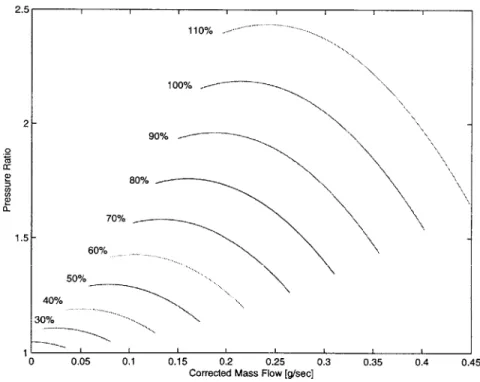
Based on the two maps for the macro-compressor and equation 2.9, four compressor maps are de-rived which will be utilized in the simulations: a hypothetical map, an adiabatic experimental map, a diabatic experimental map, and a modified diabatic experimental map. The first two maps don't consider the effects of the heat flux; the last two do. The following describes these four maps in detail.
Hypothetical Map - the First Compressor Map
The hypothetical map is the first compressor map. It comes from the macro-compressor map from the ARO review [9]. There the 42% and 100% speed lines are given. The other speed lines are obtained by extrapolation and assuming:
APC M 2
Ng2 N
where AP is the pressure rise across the compressor, N, = N/Ndesign is the percentage of the
rotation speed, m2 is the mass flow at the inlet of the compressor, function
f(.)
is taken as aquadratic function whose coefficients are obtained by fitting the given data of the 42% and 100% speed lines. The coefficients are computed off line. Also, a fixed efficiency of 0.48 is assumed. The map is shown in Fig. 2-2.
Because this map is well formularized, it is used to test the simulation code and do some analysis.
Adiabatic Experimental Map - the Second Compressor Map
The adiabatic experimental map is the experimental map for the macro-compressor provided by [3], without any modifications. It doesn't consider the effects of the heat addition on the compressor
performance. It is shown in Fig. 2-3.
The purpose of this map is to estimate the effects of heat transfer to the engine performance by comparing the results when using this map with the results when using the third map, which utilizes the same data but adds the estimated effects of heat flux.
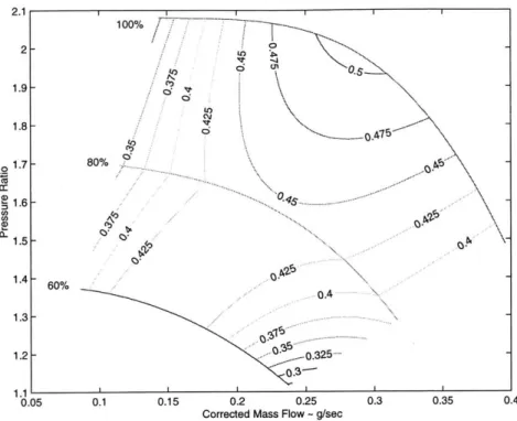
Diabatic Experimental Map - the Third Compressor Map
The diabatic experimental map is the combination of the experimental map for the macro-compressor (the second map, provided by [3]) and equation 2.9. It takes the effects of the heat flux into account. Thus it is a 3D map with the mass flow, pressure ratio and heat flux as its three dimensions. In practice the experimental data for the macro-compressor is taken as the compressor performance with 40W heat flux. The resulting 3D map is shown in Fig. 2-4. Fig. 2-5 shows an approximate 2D representation of the 3D map, with the speed lines with no heat flux as dashed lines and the speed lines with 40W heat flux as solid lines. The efficiency contours are those with 40W heat flux. Here 40W is chosen since the heat flux into the compressor at the microengine design point is around 40W. Henceforth these line types are the default line types, as listed in Table 2.1.
Table 2.1: Default Line Types for Lines with Heat Flux and without Heat Flux line type
lines with heat flux solid lines lines with no heat flux dashed lines
As mentioned before, the microengine compressor works at high Mach number and low Reynolds number, with effects of heat flux on the compressor pressure ratio and efficiency. The macro-compressors work at high Mach number and low Reynolds number, and equations 2.9 describe the effects of heat flux. Thus the third map, the diabatic experimental map, is currently the closest representation of the real microengine compressor performance.
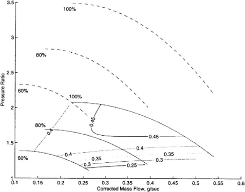
Modified Diabatic Experimental Map -the Fourth Compressor Map
Although the diabatic experimental map is currently the best approximation of the real microengine compressor performance, it takes a long time to run a single simulation. Thus the fourth map, the modified diabatic experimental map, is created to speed up the simulations without losing the basic characteristics described by the third map.
The basic idea to reduce the computation time is to replace the look-up-table operations by analytical function computations. The analytical functions are obtained by assuming ([9], [6]):
* for the speed lines,
APC nM2.
=a( a(+ -mo) 2 APo (2.10)
for all speed lines;
* for efficiency,
,)2 = (e1 N, + e2)c.
(2.11) where N, = N/Nesign, APc is the pressure rise across the compressor, z is a function of Reynolds number, APO and m0 corresponds to the highest point of 100% speed line, a, ei and e2 are constant coefficients.
In practice for speed lines, the 100% speed experimental data is used to obtain the constants
APO, mo and a, and z is computed by fitting the 80% and 60% experimental data to equation 2.10.
For efficiency, because of the relatively big measurement error during the experiment, the exper-imental efficiencies of the 60% speed line are not used. Similar to the approach used for the speed lines, coefficients ei and e2 are obtained by linear fitting of the experimental data at 100% and 80% speed to equation 2.11.
The final results for the constants are:
mo= 0.5153, APo =1.0768, z = 1.41, a = -1.6346, e= -2.4364, e2= 3.8995.
This final modified diabatic experimental map is shown in Fig. 2-6, where the default line types are used (see Table 2.1). This map was used during the parameter study and the startup process simulations, which will be described in detail in chapter 4. The simulation time for a single simulation when using this map is about 1/10 of the simulation time when using the third map, the diabatic experimental map.
Combustor
The combustor efficiency is taken as a fixed value ([9]):
qb =
Tf hr/b =m4 1 CptT4 1- m3 CcT3, (2.12)
where h is the heat value of the fuel, mf is the fuel mass flow, 7
7b is the combustor efficiency, m
4 1 and M3 are the gas mass flow at the exit and the inlet of the combustor, Cpt and Cc are the specific
heat at constant pressure of the gas at the exit and the inlet of the combustor, and T41 and T3 are
the total temperature at the exit and the inlet of the combustor.
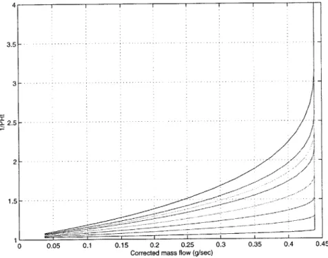
Turbine
The turbine map is obtained by extrapolation of the data at the designed point [9]. It is shown in Fig. 2-7. Here the effect of heat flux on the turbine performance is ignored, since it is expected to be very small [9].
Nozzle
Assuming an ideally expanded nozzle, the Mach number at the throat of the nozzle is related to the pressure ratio across the nozzle as:
17rn= (1+ )
where 7rn is the pressure ratio of the nozzle, Mn is the Mach number. Using mass conservation, the
nozzle is modeled as:
M45= r_ A,(1 + M )~ - -
-
M- , (2.13)where An = 5.06mm2
is the nozzle area. This value is computed by using the values of Trn, m*45, P45 and T45 at the designed point.
2.2.2
Modeling of the Dynamics
As stated in section 2.1, there are three main dynamical elements in the operation of the micro-engine: the gas dynamics, the rotor acceleration dynamics, and the heat transfer dynamics. The gas dynamics can be computed as quasi-steady values. This section models these dynamics. The combination of these dynamics models and the component models derived in the last subsection result in the nonlinear model for the microengine.
Gas Dynamics
As shown in the system diagram Fig. 2-8, first mass conservation is applied to the compressor, the combustor, and the turbine which yields the following equations:
m3
=m
2 - mbleed,m4 1=M 3 + Mrf,
m4 5=M 4 1 + bleed, (2.14)
where m3 and mr2 are the gas mass flow at the exit and inlet of the compressor, m4 5 and M4 1 are the gas mass flow at the exit and inlet of the turbine, mbleed is the bleed part of the compressor
mass flow which is injected back at the exit of the turbine, and Mif is the fuel mass flow.
Another way to obtain the mass flow into the combustor, at the turbine inlet, and at the nozzle inlet is by the pressure and the temperature, which is as follows:
P3( 3 ~ 4 1) M3-comb- kdpbT3dp 3 P41 M41_gt= M t 4 AP45 P4 5 m45-pt fn(Mn) ---
,
(2.15) VT4 5where ft(.) comes from the turbine map, and f,((M,)) comes from the nozzle model (equation 2.13). Next mass conservation is applied to each of the three infinitesimal control volumes shown in Fig. 2-8. In general, for each of these control volume, the mass conservation is as follows:
dm . .
d
=Min - mout . (2.16)dt
where m is the mass inside the control volume, min and rmot are the mass flow into the control
volume and out of the control volume, respectively. Inside the control volume, assuming a perfect gas yields:
Ps = pRTs = -RTs.
V
where V is the volume of the control volume, P, and T, are the static pressure and temperature of the gas inside the control volume, respectively. Taking the time derivative and rearranging, results in the following relation:
dm 1 dP
dt kvT dt'
where k, is a constant related to the volume.
dP
kvT(i - mout).
dt
Applying this formula to the three control volumes gives:
dP = k 3T3(m3 - m3scomb), dP41 dt = kv41T41(m*41 - m41_gt), dP45 dt kv45T45(m45 - m45-pt).
Equations 2.17 actually describes the gas As stated in section 2.1, gas dynamics the following equations hold:
dynamics.
can be computed as quasi-steady values. This means that
dP -0, dt-dP4 1 0 dt dP45 d 0. dt
Plugging equation 2.17 into them results in:
m3 =3-comb,
M4 1=M41-gt,
(2.18)
The set of equations 2.18 is one of the main sets of equations in the nonlinear model.
Rotor Acceleration Dynamics
In the microengine, the drop of enthalpy across the turbine provides power, the compressor absorbs power, and there is also some power loss due to friction, etc., which is called shaft off-take power.
So, the rotor acceleration dynamics can be described by the following equation:
dN _1
d - JN (Powert - Powere - Powershaf0), (2.19)
where J is the rotor inertia, N is the rotation speed, Powert is the power provided by the turbine,
Powere is the power absorbed by the compressor, and Powershaft is the shaft off-take power. These
three powers can be represented as:
Powerc =m2 CpcT2s"r -)/" -1
Powert =m4 1 CptT4Ji(1 -r
Powershaft = 13W x ( N)2
Ndes
The first two equations come from the definitions of the compressor and turbine efficiencies, and 13W is the shaft off-take power at design point [1].
Equation 2.19 is another main equation in the nonlinear model.
Heat Transfer Dynamics
This subsection models the heat transfer dynamics. Because of the relatively high thermal con-ductivity of silicon and the small structural scale, the rotor of the microengine has nearly uniform temperature. In the heat flux path, the major sources and sinks are the fluid across the compressor and the turbine. Here uniform rotor temperature T, is assumed and the heat sources and sinks other than the fluid across the compressor and the turbine are ignored. When analyzing the heat transfer dynamics, the rotor is taken as the object and the rotor temperature is taken as the state. Then the heat flux into the object (the rotor) is the convective heat flux from the turbine flow,
Ot,
and the heat flux out of the object is the convective heat flux into the compressor flow,QC.
Note that because the rotor is rotating, the relative temperature should be used instead of the absolute temperature when calculatingQt
andQC.
Let's first find the product of the convective heat transfer coefficient and the convective area at the turbine side and the compressor side, (hA)t and (hA)c; next derive the relationship between the relative temperature and the absolute temperature; then get the heat fluxQ
andQ;
and finally, obtain the heat transfer dynamics.Finding (hA)t and (hA)c
The convective heat transfer coefficient can be expressed as ([9]):
h = K 0.664Re1/2Pr1/3
L L
Thus with nearly the same Prandtl number and fixed area ([9]), we have:
(hA)t oc hturb oCm4 1 1/2
That is:
1/2
(hA)t = khAt n4 1
(hA)c = khAc M2 /2, (2.20)
where khAc and khAt are two constants.
[9] gives us (hA)t and (hA)c at the design point, which are as follows:
(hA)t = 0.0852W/K,
(hA)c = 0.0942W/K,
The designed mass flows are:
m4 1= 0.342g/sec,
m2= 0.36g/sec.
Then the two constants can be obtained:
khAc = 4.9648,
khAt = 4.6071. (2.21)
Equation 2.20 and 2.21 give us the formula to compute (hA)t and (hA)c.
Finding the Relationship between the Relative Temperature and the Absolute Temperature
The relationship between the total temperature and the static temperature are as follows:
Tabs = T + (Vabs)2 t = S + 2Cp
rel = T5 + (Vrel)2
tie = s + 2Cp ( 2.22)
where superscript "abs" means absolute value, superscript "rel" means relative value, subscript "t" means total, subscript "s" means static, T is the temperature, V is the gas speed, and C, is the specific heat at constant pressure.
The rotation has no radial component, and its tangential component is wR (Here W denotes the rotation speed, and R denotes the radius). Thus:
Vtan=wR- Van
After some manipulations and noting that
Va retan,ael-
V ae
where
#
is an angle determined by the blade shape.the relationship between the absolute speed and the relative speed can be expressed as:
(Vabs)2 - (grel)2 = (wR)2(1 - k, -) (2.23)
wR where kt is a constant.
Plugging equation 2.23 into equation 2.22 results in the following:
ab trl=(wR)2 m
AT =T/ab -T T' = ((1 - kt r.
2C, wR
Applying this formula to both the inlet and the outlet of the compressor and the turbine yields the
following equations: AT -( Trel wR2)2 M2 2 2 2 2Cpc (1 - kt2 w R ), 2 AT3 Tbs et (wR3 (wR3)2Rm)2 (1 - _M3 AT41 Tb - '' = R4 (1 - k i 4 1 2Cpc wR 4
(wR
41)2 mn41 AT45 E T5as* - T5Re = 5 (1 - kt45 ), (2.24) 2Cpt wR 45where R2, R3, R4 1 and R45 are the radius of the inlet and the outlet of the compressor and the
turbine, respectively.
The differences of the absolute and relative temperatures at designed point at both the inlet and the outlet of the compressor and the turbine are given by [9], which are as follows:
AT2 = -62K,
AT3 = -31K,
AT4 1 = 107K,
The radius of the inlet and the outlet of the compressor and the turbine are ([9]):
R2 = 2.00mm,
R3 = 4.00mm,
R41= 2.52mm, R45 = 1.50mm.
Combining the above data with the other parameters at the design point, the constant kt at the different stations can be obtained as:
kt2 = 1.0373e6
kt3 = 0.8704e6
kt41 =-0.8999e6
kt45 0.5111e6 (2.25)
Equation 2.24 and 2.25 give us the relationship between the relative temperatures and the ab-solute temperatures at both the inlet and the outlet of the compressor and the turbine.
Heat Flux into the Compressor and Heat Flux out of the Turbine
Precise values for the convective heat flux
Q
andQt
would be found by integrating the heat flux of each infinitesimal piece along the compressor and the turbine, respectively. Here for simplicity the "characteristic temperatures" T , and T[j6 are used to calculateQc
and Qt, i.e.:.c= (hA)c(Tw - T l
Qt=
(hA)t(Ttur - Tw). (2.26)The characteristic temperature Tcr,, is taken as the average of the relative temperatures at the inlet and the outlet of the compressor, and the characteristic temperature Te4 is taken as the average
of the relative temperatures at the inlet and the outlet of the turbine, as follows:
TCOMP (T2' + T )e/}2,
T[rb = (Tf' + Til) /2. (2.27)
equation 2.27 yields the following:
Trek, = [(Tabs + Tib") - (AT2 + AT3)],
TtI =b -[(TL"s + TjoS) - (AT4 1 + AT4 5)]. (2.28)
2
Equations 2.26 and 2.28 show that
Q
andQ
are functions of (hA), (hA)t and absolutetemperatures. Equations 2.20 shows that (hA)c and (hA)t are functions of mass flow and rotation speed. Equations 2.24 show that the differences between the absolute temperatures and the relative temperatures are also functions of mass flow and rotation speed. Thus
Qc
andQt
are functions of mass flow, absolute temperatures and rotation speed. In addition, compressor mass flow is a function ofQc
(the compressor map is a 3D map withQc
as one of its dimensions). Absolute temperatures are also functions ofQc
andOt,
as follows:m2 Cpc(Tb"s - Tbs) = Workc+ Qc,
m4 1 C-(T " T4S) Workt+
Q
. (2.29)where Workt and Workc are adiabatic work of the compressor and the turbine:
Workc =m 2 CpcTjbs(-i)/T( -1r
(-yt -l1)/ytt
Workt =m41 CpT 1 s(1 - rt. (2.30)
Thus these equations (equation 2.20, 2.24, 2.26, 2.28, 2.29, and 2.30), along with the compressor map, are highly coupled nonlinear equations. Solving these equations simultaneously can give us
OC
and Qt.
Heat Transfer Dynamics
Knowing
Q
andQt,
the heat transfer dynamics can be found. The net heat flux flowing into the rotor is:Q=Q
-
Q.
(2.31)Applying energy conservation to the rotor results in:
dTw
Q= CWMW dt (2.32)
where C, and M. are the specific heat and the mass of the rotor, respectively. Combining equation 2.31 and equation 2.32 yields the following:
dT O- - O
d t
Q t - Q(2
M .3 3 )dt CWMW
This is the equation which describes the dynamics of the state Tw, i.e. the heat transfer dynamics.
2.2.3
Nonlinear Model Simulator
The above two subsections give us the nonlinear model, which is mainly described by equations 2.18, 2.19 and 2.33, combined with the component models and equations 2.14, 2.15, 2.20, 2.24, 2.26, 2.28, 2.29, and 2.30. This subsection describes the nonlinear model simulator.
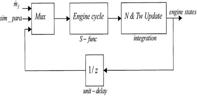
The diagram of the simulator is shown in Fig. 2-9. As shown in the figure, the inputs are the fuel flow myf, the simulation parameters like the error tolerance, and the initial states of the engine. The outputs are the engine states at every time step. The integration of the rotor speed for the unbalanced powers and the rotor temperature for the unbalanced heat flux (correspond to equation 2.19 and 2.33) are solved in the "N and Tw update" block. Thus the "engine cycle" block is static; i.e., it does not include dynamical states. The task of the "engine cycle" block is to generate the quasi-static solutions for the gas dynamics (equations 2.18, 2.14 and 2.15) and the heat flux Q
and Q (equations 2.20, 2.24, 2.26, 2.28, 2.29, and 2.30). Here a Lipschitz numerical approach is used to solve these highly coupled and nonlinear equations.
In practice, the simulator is accomplished by Simulink in MATLAB [11]. The "engine cycle" block is accomplished by an S-function [11] written in C. The code for the S-function is attached in the Appendix. Since the "engine-cycle" block is a little complicated, the following says a little more about the operations in this block.
"Engine Cycle" Block
As stated before, the quasi-static solutions for the gas dynamics (equations 2.18, 2.14 and 2.15) and the heat flux Q and Qt (equations 2.20, 2.24, 2.26, 2.28, 2.29, and 2.30) are generated in the "engine cycle" block. The Lipschitz numerical approach is used to solve these highly coupled and nonlinear equations. The follows first describes how the Lipschitz numerical approach works, then applies it to the problem, and finally describes the steps in the "engine cycle" block.
Basically, the Lipschitz approach is a recursive solution procedure. In this approach one first sets initial values for the unknowns. The next estimates for the unknowns are modifications of the previous estimates. In general, assume the equation to be solved is:
x =