HAL Id: hal-03225838
https://hal.archives-ouvertes.fr/hal-03225838
Submitted on 16 May 2021
HAL is a multi-disciplinary open access
archive for the deposit and dissemination of
sci-entific research documents, whether they are
pub-lished or not. The documents may come from
teaching and research institutions in France or
abroad, or from public or private research centers.
L’archive ouverte pluridisciplinaire HAL, est
destinée au dépôt et à la diffusion de documents
scientifiques de niveau recherche, publiés ou non,
émanant des établissements d’enseignement et de
recherche français ou étrangers, des laboratoires
publics ou privés.
site-level data to evaluate Earth system models
Sarah Chadburn, Gerhard Krinner, Philipp Porada, Annett Bartsch,
Christian Beer, Luca Belelli Marchesini, Julia Boike, Altug Ekici, Bo
Elberling, Thomas Friborg, et al.
To cite this version:
Sarah Chadburn, Gerhard Krinner, Philipp Porada, Annett Bartsch, Christian Beer, et al.. Carbon
stocks and fluxes in the high latitudes: using site-level data to evaluate Earth system models.
Bio-geosciences, European Geosciences Union, 2017, 14 (22), pp.5143-5169. �10.5194/bg-14-5143-2017�.
�hal-03225838�
https://doi.org/10.5194/bg-14-5143-2017 © Author(s) 2017. This work is distributed under the Creative Commons Attribution 3.0 License.
Carbon stocks and fluxes in the high latitudes: using site-level
data to evaluate Earth system models
Sarah E. Chadburn1,2, Gerhard Krinner3, Philipp Porada4,5, Annett Bartsch6,7, Christian Beer4,5, Luca Belelli Marchesini8,9, Julia Boike10, Altug Ekici11, Bo Elberling12, Thomas Friborg12, Gustaf Hugelius13,
Margareta Johansson14, Peter Kuhry13, Lars Kutzbach15, Moritz Langer10, Magnus Lund16,
Frans-Jan W. Parmentier17,20, Shushi Peng3,18, Ko Van Huissteden9, Tao Wang19, Sebastian Westermann20, Dan Zhu21, and Eleanor J. Burke22
1University of Leeds, School of Earth and Environment, Leeds LS2 9JT, UK
2University of Exeter, College of Engineering, Mathematics and Physical sciences, Exeter EX4 4QF, UK 3CNRS, University Grenoble Alpes, IGE, Grenoble, France
4Department of Environmental Science and Analytical Chemistry, Stockholm University, 10691 Stockholm, Sweden 5Bolin Centre for Climate Research, Stockholm University, 10691 Stockholm, Sweden
6Department of Geodesy and Geoinformation, Vienna University of Technology, Vienna, Austria 7Cryosphere & Climate, Austrian Polar Research Institute, Vienna, Austria
8School of Natural Sciences, Far Eastern Federal University, Vladivostok, Russia 9Department of Earth Sciences, Vrije Universiteit (VU), Amsterdam, the Netherlands
10Alfred Wegener Institute, Helmholtz Centre for Polar and Marine Research (AWI), 14473 Potsdam, Germany 11Uni Research Climate and Bjerknes Centre for Climate Research, Bergen, Norway
12Center for Permafrost (CENPERM), Department of Geosciences and Natural Resource Management, University of Copenhagen, Copenhagen, Denmark
13Department of Physical Geography, Stockholm University, 10691 Stockholm, Sweden
14Department of Physical Geography and Ecosystem Science, Lund University, Sölvegatan 12, 223 62 Lund, Sweden 15Institute of Soil Science, Center for Earth System Research and Sustainability, Universität Hamburg, Hamburg, Germany 16Department of Bioscience, Arctic Research Center, Aarhus University, Frederiksborgvej 399, 4000 Roskilde, Denmark 17Department of Arctic and Marine Biology, UiT – The Arctic University of Norway, Tromsø, Norway
18Sino-French Institute for Earth System Science, College of Urban and Environmental Sciences, Peking University, Beijing 100871, China
19Key Laboratory of Alpine Ecology and Biodiversity, Institute of Tibetan Plateau Research and Center for Excellence in Tibetan Plateau Earth Sciences, Chinese Academy of Sciences, Beijing 100085, China
20University of Oslo, Department of Geosciences, P.O. Box 1047 Blindern, 0316 Oslo, Norway
21Laboratoire des Sciences du Climat et de l’Environnement, LSCE CEA CNRS UVSQ, Gif-Sur-Yvette, France 22Met Office Hadley Centre, Fitzroy Road, Exeter EX1 3PB, UK
Correspondence to:Sarah E. Chadburn (s.e.chadburn@exeter.ac.uk) Received: 17 May 2017 – Discussion started: 31 May 2017
Abstract. It is important that climate models can accu-rately simulate the terrestrial carbon cycle in the Arctic due to the large and potentially labile carbon stocks found in permafrost-affected environments, which can lead to a pos-itive climate feedback, along with the possibility of future carbon sinks from northward expansion of vegetation under climate warming. Here we evaluate the simulation of tun-dra carbon stocks and fluxes in three land surface schemes that each form part of major Earth system models (JSBACH, Germany; JULES, UK; ORCHIDEE, France). We use a site-level approach in which comprehensive, high-frequency datasets allow us to disentangle the importance of different processes. The models have improved physical permafrost processes and there is a reasonable correspondence between the simulated and measured physical variables, including soil temperature, soil moisture and snow.
We show that if the models simulate the correct leaf area index (LAI), the standard C3 photosynthesis schemes pro-duce the correct order of magnitude of carbon fluxes. There-fore, simulating the correct LAI is one of the first priorities. LAI depends quite strongly on climatic variables alone, as we see by the fact that the dynamic vegetation model can simulate most of the differences in LAI between sites, based almost entirely on climate inputs. However, we also iden-tify an influence from nutrient limitation as the LAI becomes too large at some of the more nutrient-limited sites. We con-clude that including moss as well as vascular plants is of pri-mary importance to the carbon budget, as moss contributes a large fraction to the seasonal CO2flux in nutrient-limited conditions. Moss photosynthetic activity can be strongly in-fluenced by the moisture content of moss, and the carbon up-take can be significantly different from vascular plants with a similar LAI.
The soil carbon stocks depend strongly on the rate of in-put of carbon from the vegetation to the soil, and our anal-ysis suggests that an improved simulation of photosynthe-sis would also lead to an improved simulation of soil carbon stocks. However, the stocks are also influenced by soil car-bon burial (e.g. through cryoturbation) and the rate of het-erotrophic respiration, which depends on the soil physical state. More detailed below-ground measurements are needed to fully evaluate biological and physical soil processes. Fur-thermore, even if these processes are well modelled, the soil carbon profiles cannot resemble peat layers as peat accumu-lation processes are not represented in the models.
Thus, we identify three priority areas for model devel-opment: (1) dynamic vegetation including (a) climate and (b) nutrient limitation effects; (2) adding moss as a plant functional type; and an (3) improved vertical profile of soil carbon including peat processes.
1 Introduction
Land areas in northern high latitudes may represent a net source or a net sink of carbon to the atmosphere in the fu-ture, and there is not yet a consensus as to which of the two is more likely (Cahoon et al., 2012; Hayes et al., 2011). This is not because it is likely to be small: on a pan-Arctic scale we could see anything between a net emission of over 100 Gt C or a net sink of up to 60 Gt C by the end of this century (Schuur et al., 2015; Qian et al., 2010). To put this into context, the remaining emissions budget in order to sta-bilise climate warming below 2◦C above pre-industrial lev-els is less than 250 Gt C from 2017 on (Peters et al., 2015). Thus, it is very important to reduce uncertainty in the north-ern high latitude carbon cycle. The uncertainty comes largely from the representation of these processes in Earth system models (ESMs), which are our main tool for future climate projections.
The potential for large carbon emissions comes from the large quantities of old carbon that are frozen into permafrost, protected from decomposition under the current cold climate. Around 800 Gt of carbon is stored in permanently frozen soils (Hugelius et al., 2014). If the permafrost thaws, this carbon may decompose and be released into the atmosphere (Burke et al., 2012, 2013; Koven et al., 2015; Schneider von Deimling et al., 2012, 2015; MacDougall and Knutti, 2016). Conversely, the increased vegetation growth that is already taking place in the Arctic under climate warming (Tucker et al., 2001; Tape et al., 2006) could result in a net uptake of carbon from the atmosphere (Quegan et al., 2011; Qian et al., 2010). It should be noted, however, that in some areas Arctic vegetation growth is not increasing but rather “brown-ing” (Epstein et al., 2016).
The representations of both permafrost carbon and Arc-tic vegetation in ESMs are not well developed. Some mod-els now include a vertical representation of soil carbon, which allows the frozen carbon in permafrost to be included (Koven et al., 2009, 2013; Schaphoff et al., 2013; Burke et al., 2017), but most do not yet represent important mech-anisms of carbon storage and release, such as sedimenta-tion, thermokarst formation and a proper representation of cryoturbation (Schneider von Deimling et al., 2015; Beer, 2016), although sedimentation is included in (Zhu et al., 2016). There is also a growing consensus that the chemical decomposition models used in ESMs are not adequate to rep-resent microbial processes (Wieder et al., 2013; Xenakis and Williams, 2014). Vegetation models also, for the most part, do not include the appropriate high-latitude vegetation types, and those models that have dynamic vegetation are lacking in processes that are essential determinants of vegetation dy-namics, such as nutrient limitation and interactions with soil (Wieder et al., 2015).
In this paper we assess the ability of the land surface com-ponents from three ESMs to represent the carbon stocks and fluxes observed at tundra sites, identifying the processes that
have the greatest impact on the uncertainty. These processes are therefore priorities for future model development. Ob-servational studies in tundra environments have shown that carbon dynamics are sensitive to physical conditions (Lund et al., 2012; Cannone et al., 2016; Pirk et al., 2017); thus, we first assess the ability of the models to capture the mean physical state of the system and the differences between sites, specifically in terms of snow depth, soil temperature, soil moisture and active-layer depth. Secondly, soil carbon stocks are evaluated against measured soil carbon profiles, assess-ing the main causes of biases in the models. Half-hourly net ecosystem exchange (NEE) data from eddy flux towers are used to evaluate the simulated carbon fluxes, comparing the models directly against observations before analysing the re-lationships between ecosystem carbon fluxes and different driving variables. We also consider the impacts of other con-trolling factors such as nutrient limitation and mosses, whose importance has been identified in previous studies (Atkin, 1996; Uchida et al., 2009).
This is a synthesis from the recently concluded EU project PAGE21 (Changing Permafrost in the Arctic and its Global Effects in the 21st century), evaluating the models that took part in the project (described in Sect. 2.2, below) at the five PAGE21 primary sites, which are all located in Arctic per-mafrost regions, specifically Siberia, Sweden, Svalbard and Greenland. After the site-level evaluation of physical pro-cesses by (Ekici et al., 2015), this evaluation of carbon cycle processes continues site-level model evaluation efforts. The sites are described in detail in Sect. 2.3.
2 Methods
This study takes three different angles: (1) comparison with observed indicators; (2) comparison of processes between models and (3) comparison of geographical conditions (e.g. vegetation, permafrost) between sites. The structure of the methods section is as follows: first describing the observa-tional indicators used (Sect. 2.1), second the processes rep-resented in the models (Sect. 2.2) and third the conditions at the sites (Sect. 2.3). Lastly, details of the simulation set-up and forcing data are given in Sect. 2.4.
2.1 Evaluation data 2.1.1 Carbon dioxide flux
Eddy covariance half-hourly CO2flux data and related me-teorological variables used in this study are archived in the PAGE21 fluxes database (http://www.europe-fluxdata.eu/ page21), which is part of the European Fluxes Database Cluster.
Flux post-processing was performed consistently for all the sites following the protocol applied for the FLUXNET2015 data release (http://fluxnet.fluxdata.org/ data/fluxnet2015-dataset), with customised choices of the
processing options. The applied scheme included the follow-ing: (i) a quality assessment and quality control procedure over single variables aimed at detecting implausible values or incorrect time stamps (e.g. by comparing patterns of poten-tial and observed downward shortwave radiation at a given location); (ii) the computation of NEE by adding the CO2 flux storage term calculated from a single CO2 concentra-tion measurement point (at the top of the flux tower) and assuming a vertically uniform concentration field; (iii) the de-spiking of NEE based on (Papale et al., 2006) using a threshold value (z = 5); (iv) NEE filtering according to an ensemble of friction velocity (u∗) thresholds obtained with bootstrapping following the methods of (Barr et al., 2013) and (Papale et al., 2006) and selection of a u∗threshold, dif-ferent for each year, based on the highest model efficiency (Nash–Sutcliffe); (vi) the gap-filling of NEE time series with the marginal distribution sampling method (Reichstein et al., 2005).
Finally, NEE was partitioned into the gross primary pro-ductivity (GPP) and ecosystem respiration (Reco) compo-nents using a semi-empirical model based on a hyperbolic light-response curve fitted to daytime NEE data (Lasslop et al., 2010). The years of data available for each site are given in Table S1.
2.1.2 Soil carbon profiles
Typical soil profiles with data on soil organic carbon content were generated for each site. Based on extensive field cam-paigns in each study area, individual pedons for representa-tive landscape and soil types were combined and harmonised. In brief, soils were classified and sampled from open soil pits dug down to the permafrost. Permafrost samples were collected through manual coring into the permafrost at the bottom of the soil pit. In most cases, soils were sampled to a depth of 1 m. The harmonised soil profiles were generated by averaging several soil pedons per landscape type at a 1 cm depth resolution. For more detailed descriptions of field sam-pling and laboratory procedures, see Palmtag et al. (2015) and Siewert et al. (2015, 2016). Top 1 m total soil carbon values were calculated from a weighted average of different typical profiles, based on the fractional coverage of landscape types in the footprint area of the flux towers.
2.1.3 Snow depth
Snow depth was recorded using automatic sensors (except Abisko, where it is manual). Snow depth from the Abisko mire (Storflaket) was recorded manually monthly (Johans-son et al., 2013). Snow depth at Samoylov and Bayelva was recorded hourly, and for Zackenberg 3-hourly (using sonic range and laser sensors). Snow depth at Kytalyk was mea-sured by means of a 70 cm vertical profile made of thermis-tors spaced every 5 cm (2.5 cm between 0 and 10 cm height from the ground). Data were logged every 2 h and the snow–
air interface level was identified by analysing the profile pat-terns with a MATLAB© routine calibrated to search for devi-ations between consecutive resistance readings above a given threshold. Years used for each site are given in Table S1. 2.1.4 Soil temperature
For Samoylov, Bayelva, Kytalyk and Zackenberg, soil tem-perature was recorded hourly using thermistors (Kytalyk set-up described in van der Molen et al., 2007). Ground temper-atures for Abisko mire were recorded at the Storflaket mire, at boreholes cased with plastic tubes and instrumented with HOBO loggers U12 (industry, four channels) together with HOBO soil temperature sensors (Johansson et al., 2011). The years used for each site are given in Table S1.
2.1.5 Soil moisture
Continuous soil moisture measurements are only available for Bayelva, Samoylov and Zackenberg. At Samoylov and Bayelva, hourly volumetric soil water content was recorded (using time domain reflectometry). At Zackenberg soil moisture was measured using permanently installed ML2x ThetaProbes (Lund et al., 2014). Years used for each site are given in Table S1. Indicative soil moisture levels for Abisko mire were collected from May to October 2015 (Pedersen et al., 2017), measured manually as volumetric soil water content integrated over 0–6 cm depth using a handheld ML2x ThetaProbe (Delta-T Devices Ltd., Cambridge, UK). Soil moisture was measured five times in each plot and averages were subsequently used.
2.1.6 Active-layer depth
Active-layer depth was measured at Circumpolar Active Layer Monitoring (CALM) grids at most of the sites. At Bayelva there is no CALM grid; thus, the active layer was estimated from soil temperature measurements and is given as an indicative value. Active-layer thickness monitoring is determined by mechanical probing. A 1 cm diameter gradu-ated steel rod is inserted into the soil to the depth of resis-tance to determine the active-layer thickness (Åkerman and Johansson, 2008) according to the CALM standard.
2.1.7 Leaf area index
Leaf area index was taken from the MODIS product (MODIS15A2, 2016) for the closest coordinates to the sites. This product has been successfully applied to tundra sites (Cristóbal et al., 2017). It was evaluated by (Cohen et al., 2006), who found an RMSE of 0.28 at a tundra site. There are, however, still considerable uncertainties in using this data product (see Sect. 3.6.1).
2.1.8 GPP per unit leaf area
This was calculated using the partitioned GPP from the eddy covariance data (Sect. 2.1.1), averaged daily and taken on the same day as the values from the MODIS LAI product (Sect. 2.1.7). Note that there are no time-resolved GPP val-ues for Bayelva due to insufficient data. The extracted GPP values were divided by the appropriate LAI estimates and the resulting values were collected for all sites and binned into intervals of air temperature (1.5◦C) and shortwave radiation (20 Wm−2), for which the mean and standard deviation were then calculated (shown in Fig. 9).
2.2 Model description
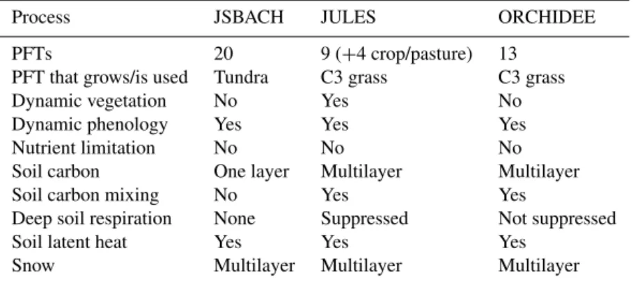
The three models studied here are JSBACH (Jena Scheme for Biosphere–Atmosphere Coupling in Hamburg; Raddatz et al., 2007; Brovkin et al., 2009), JULES (Joint UK Land Environment Simulator; Best et al., 2011; Clark et al., 2011) and ORCHIDEE (ORganizing Carbon and Hydrology In Dy-namic Ecosystems Environment; Krinner et al., 2005). These are all land surface components of major ESMs (JSBACH: MPI-ESM; JULES: UKESM; ORCHIDEE: IPSL). Key fea-tures are summarised in Table 1.
These models can be run in a coupled mode within the ESM, or, as here, they can be run as stand-alone models forced by observed meteorology. The models are run as a gridded set of points for large-scale simulations, and they can also be run for single points, as in this study. Each model had some development of high-latitude processes during the PAGE21 project, and model developments have also been on-going since the conclusion of the project in late 2015.
All the models simulate vertical fluxes of water, heat and carbon between the atmosphere, the vegetation and the soil. Of relevance to permafrost physics, the models simulate a dy-namic snowpack by means of a multilayer snow scheme and the freezing and thawing of soil (Ekici et al., 2014; Gouttevin et al., 2012a; Wang et al., 2013; Best et al., 2011). All models use a vertical discretisation of soil thermal and hydrological fluxes, with differing resolutions (see Appendix Table A2). JSBACH has the lowest-resolution soil, with only five lay-ers in the top 10 m (Hagemann and Stacke, 2015), although in this latest version it is extended to 50 m depth with addi-tional layers. ORCHIDEE and JULES also simulate an extra thermal-only column at the base of the hydrological column to represent bedrock (Chadburn et al., 2015a).
Soil thermal and hydrological properties in both JULES and ORCHIDEE have been adapted to allow better repre-sentation of organic soils, whereas in JSBACH only min-eral soil properties are represented. However, JSBACH ad-ditionally simulates a moss and/or lichen layer at the surface with dynamic moisture contexts and thermal properties (Po-rada et al., 2016), which physically represents the surface or-ganic layer. Oror-ganic soil properties in JULES are described in Chadburn et al. (2015a). In ORCHIDEE the scheme
fol-lows (Lawrence and Slater, 2008), using the observation-based soil carbon map from (Hugelius et al., 2014).
Soil carbon is represented by a multi-pool scheme in all the models, with inputs from vegetation, and decomposition rates depending on soil temperature, soil moisture and intrin-sic turnover times of different pools (Goll et al., 2015; Clark et al., 2011). Both ORCHIDEE and JULES represent a verti-cal profile of soil carbon (discretised in line with the soil hy-drology), including cryoturbation mixing (Koven et al., 2009; Burke et al., 2017). JSBACH, however, represents only a sin-gle layer, with decomposition rates determined by conditions in the upper layer of soil.
None of the models simulate nitrogen or other nutrients. Vegetation growth and productivity is therefore only deter-mined by soil moisture and atmospheric forcing data, with no nutrient limitation. Different land cover types are repre-sented in the models by surface tiles, which can vary in frac-tional cover. In JULES, a dynamic vegetation model is run with nine competing plant functional types (PFTs) (Harper et al., 2016), whereas in the other models, vegetation is fixed, but with dynamic phenology. ORCHIDEE has 13 PFTs but there is no specific high-latitude PFT in the version used here; thus, C3 grasses are prescribed for these sites. In JS-BACH there are 20 PFTs (including crop and pasture) and for these sites a tundra PFT is used, which is similar to C3 grass but with reduced Vcmax (maximum rate of carboxy-lation in leaves). In JSBACH there is also a dynamic moss model simulating moss photosynthesis and respiration, as in the model described by (Porada et al., 2013). This model rep-resents both mosses and lichens by one plant functional type with average physiological properties. In the version used here, the moss carbon fluxes are not yet fully coupled into the JSBACH carbon cycle; thus, the moss carbon fluxes are considered separately in the analysis that follows.
For more details of the soil and vegetation configuration see Sect. 2.4 and the Appendix.
2.3 Site descriptions
The sites represent a range of climatological and biogeophys-ical conditions across the tundra. Abisko is the warmest site, with sporadic permafrost, followed by Bayelva, which is a high Arctic maritime site (on Svalbard), and Zackenberg, which is a maritime site in Greenland (colder than Bayelva). Samoylov and Kytalyk have a continental Siberian climate and the coldest mean annual temperatures. The landscapes differ between sites, which can influence the permafrost and carbon dynamics, for example through the impact of topogra-phy on snow distribution and hydrology. The following sec-tions provide a short description of each study area, and the important climatic and permafrost variables are given in Ta-ble 2.
At all sites there has been some tendency towards air tem-perature warming, which in many cases is accompanied by warming or thawing of permafrost (Callaghan et al., 2010;
Christiansen et al., 2010; Parmentier et al., 2011; Boike et al., 2013; Lund et al., 2014; Abermann et al., 2017).
2.3.1 Abisko
The Abisko site is located in the Torneträsk catchment in northernmost Sweden. According to (Brown et al., 1998), the Abisko area lies within the zone of discontinuous per-mafrost. However, with the observed permafrost degradation during the last decades (Åkerman and Johansson, 2008; Jo-hansson et al., 2011), the area is now more characteristic of the sporadic permafrost zone. Permafrost is widespread in the mountains (Ridefelt et al., 2008), but at lower ele-vations permafrost is only found in peat mires (Johansson et al., 2006). Data from three sites from the Torneträsk catch-ment (within an area of 10 km) have been used for this study. The principal sites are Storflaket and Stordalen peat mires. The active-layer measurements and the ground temperatures are monitored at the Storflaket site (Åkerman and Johansson, 2008; Johansson et al., 2011) and the carbon monitoring, in-cluding the eddy covariance measurement, is carried out at the Stordalen site. These two mire sites are very similar in terms of climate, soil profile and permafrost characteristics. The footprint of the eddy covariance tower is characterised by wet fen with no permafrost present and vegetation dom-inated by tall graminoids (Jammet et al., 2015, 2017). For comparison, additional soil temperature data from a mineral soil site at the Abisko Scientific Research Station, which is not underlain by permafrost, are included.
2.3.2 Bayelva (Svalbard)
The study site is located in the high-Arctic Bayelva River catchment area, close to Ny-Ålesund on Spitsbergen island in the Svalbard archipelago. The area is characterised by mar-itime continuous permafrost. In bioclimatic terms the area represents a semi-desert ecosystem (Uchida et al., 2009). Vegetation includes low vascular plants (mainly grass, sedge, catchfly, saxifrage and willow), mosses and lichens (Oht-suka et al., 2006; Uchida et al., 2006). The ground is mostly bedrock but is partly covered by a mixture of sediments. The study site is located on permafrost patterned ground mainly consisting of non-sorted soil circles or mud boils, with around 60 % vegetation cover. The eddy covariance measure-ments were conducted on Leirhaugen hill, and additional me-teorological observations and ground temperature measure-ments are continuously conducted at the Bayelva soil and cli-mate monitoring station (Boike et al., 2003, 2008a; Roth and Boike, 2001) 100 m away. Over the past decade the Bayelva catchment has been the focus of intensive investigations on soil and permafrost conditions (Roth and Boike, 2001; Boike et al., 2008a; Westermann et al., 2010, 2011) and the surface energy balance (Boike et al., 2003; Westermann et al., 2009). Details of the measurements are provided in Westermann et al. (2009) and Lüers et al. (2014).
2.3.3 Kytalyk
The Kytalyk site is located in the Kytalyk reserve, 28 km northwest of the village of Chokurdakh in the Republic of Sakha (Yakutia), Russian Federation. The site is located be-tween the East Siberian Sea and the transition zone bebe-tween taiga and tundra. The area is underlain by continuous per-mafrost. The measurement site is located at the bottom of a drained former thermokarst lake, and the site is bordered by the edge of the present river floodplain. Both on the flood-plain and at the lake bottom, a network of ice wedge poly-gons occurs, in general of the low-centred type. These form a mosaic of low plateaus and ridges dominated by Betula nanaand diffuse drainage channels covered with a meadow-like vegetation of Eriophorum angustifolium and Carex sp. There is also hummocky Sphagnum with low Salix dwarf shrubs, polygon ponds covered with mosses and Comarum palustre, deeper ponds in which ice wedges have thawed, and drier areas covered with Eriophorum vaginatum tussocks. The soils generally have a 10–40 cm organic top layer overly-ing silt. The eddy covariance tower is located at a distance of ca. 200 m from the research station buildings (van der Molen et al., 2007). The tower footprint covers a wet northwestern and southeastern sector dominated by Sphagnum and ponds, while the northeastern and southwestern sectors have drier vegetation types.
2.3.4 Samoylov
Samoylov Island lies within one of the main river chan-nels in the southern part of the Lena river delta in north-ern Yakutia. The landscape on Samoylov Island, and in the delta as a whole, has generally been shaped by water through erosion and sedimentation (Fedorova et al., 2015), and by thermokarst processes (Morgenstern et al., 2013). Contin-uous cold permafrost underlies the study area to between about 400 and 600 m below the surface. The terrace where the study site is situated is covered in low-centred ice wedge polygons, with water-saturated soils or small ponds in the polygon centres. The mineral soil is generally sandy loam, underlain by silty river deposits, with a ∼ 30 cm thick or-ganic layer (Boike et al., 2013). Vegetation in the polygon centres and at the edge of ponds is dominated by sedges and mosses, and at the polygon rims various mesophytic dwarf shrubs, forbs and mosses dominate (Kutzbach et al., 2007). It is estimated that moss contributes around 40 % to the to-tal photosynthesis (Kutzbach et al., 2007). Detailed informa-tion concerning the climate, permafrost, land cover, vegeta-tion and soil characteristics of Samoylov Island can be found in (Boike et al., 2013) and (Morgenstern et al., 2013). Anal-ysis of the energy balance for the site is found in Boike et al. (2008b) and Langer et al. (2011a, b).
2.3.5 Zackenberg
The Zackenberg study site is located near the Zackenberg Re-search Station within the Northeast Greenland National Park, within the continuous permafrost zone. High mountains sur-round the Zackenberg valley to the west, east and north, with a fjord to the south, and snow cover is characterised by large interannual variability (Pedersen et al., 2016). Water avail-ability is thus regulated by topography and snow distribution patterns. Most vegetation in the Zackenberg valley is located below 300 m a.s.l., where the lowland is dominated by non-calcareous sandy fluvial sediments (Elberling et al., 2008), and peat soils have limited spatial coverage (Palmtag et al., 2015). The study site is located within a Cassiope tetragona tundra heath, dominated by C. tetragona, Dryas integrifolia and Vaccinium uliginosum, with patches of mosses. Several studies on soil and permafrost (Palmtag et al., 2015; West-ermann et al., 2015), surface energy balance (Lund et al., 2014; Stiegler et al., 2016; Lund et al., 2017) and carbon exchange (Mastepanov et al., 2008; Lund et al., 2012; Elber-ling et al., 2013) have been published based on data from this site. A rich dataset is available from this site through the ex-tensive, cross-disciplinary Greenland Ecosystem Monitoring programme (www.g-e-m.dk).
2.4 Simulation set-up
The sites were represented in all the models by a single ver-tical column, although there was some horizontal represen-tation by means of tiling approaches (see model description, Sect. 2.2). The models were run in the most up-to-date con-figurations, including new permafrost-relevant model devel-opments where available. Variables were output at hourly and/or daily resolutions.
The meteorological driving data were prepared using ob-servations from the site combined with reanalysis data for the grid cell containing the site. For the period 1901–1979, Water and Global Change forcing data (WFD) were used (Weedon et al., 2011). Data are provided at half-degree res-olution for the whole globe at 3-hourly time resres-olution from 1901 to 2001. For the period 1979–2014, WATCH-Forcing-Data-ERA-Interim (WFDEI) was used (Weedon, 2013). For the time periods in which observed data were available, cor-rection factors were generated by calculating monthly biases relative to the WFDEI data. These corrections were then ap-plied to the time series from 1979 to 2014 of the WFDEI data. The WFD before 1979 were then corrected to match these data and the two datasets were joined at 1979 to provide gap-free 3-hourly forcing from 1901 to 2014. Local meteo-rological station observations were used for all variables ex-cept snowfall, which was estimated from the observed snow depth by treating increases in snow depth as snowfall events with an assumed snow density (see Appendix). These re-constructions were then used to provide correction factors to WFDEI and WFD. This leads to a more realistic snow depth
in the model than using direct precipitation measurements, which are less precise due to wind effects and the difficulty of accurately measuring snowfall. However, the local pre-cipitation measurements were still used for rainfall, as this is much more reliable, with a potential undercatch of only around 10 % (Yang et al., 2005). For Abisko, meteorolog-ical data from the research station were used but addition-ally corrected by scaling the snowfall according to the ratio of monthly snow depths at the mire vs. the research station (snow depth was only measured monthly at Storflaket mire), and a reduction of 1◦C in air temperature. Even with these corrections, there is still considerable uncertainty in precip-itation forcing, particularly the snowfall, so in order to test the impact of this, two of the models (JULES and JSBACH) performed two additional sets of simulations, with snowfall increased and reduced by 50 %.
Spin-up was performed as consistently as possible be-tween the models, using the meteorological forcing from 1901 to 1930. Years were selected at random from this 30-year period and the models were run for 10 000 years with pre-industrial CO2levels (1850, 286 ppm), followed by 50 years with changing CO2levels (1851–1900). The model state at the end of this spin-up period was taken as the initial state for the main run (1 January 1901 to 31 December 2013). For JSBACH, there was an initial 50 years of hydrological spin-up before the main spin-up, with the permafrost impact on hydrology switched off, to allow the water to form a re-alistic profile (permafrost layers are impermeable and thus unrealistic initial conditions could otherwise be preserved). For JSBACH, the long spin-up was also between 7000 and 8000 years rather than 10 000 since in this model there is no vertical representation of soil carbon, and therefore the soil carbon pools equilibrate much more quickly and had reached a steady state after 7000–8000 years. The CO2forcing data are from (Meinshausen et al., 2011).
The soil parameters in the models were set up to repre-sent each site as closely as possible (see Appendix and Ta-ble A1). These drew from literature values, a PAGE21 de-liverable “catalogue of physical parameters”, and field ex-perience. (Note that the soil carbon profiles described in Sect. 2.1.2 were not used for this).
Vegetation was prescribed in ORCHIDEE and JSBACH. Since these are tundra sites, JSBACH used a tundra PFT (100 % coverage), which is similar to C3 grass but with re-duced Vcmax. ORCHIDEE prescribed C3 grass (100 % cov-erage) as there is no tundra PFT in this model version. JULES was run with dynamic vegetation using nine PFTs (Harper et al., 2016), which do not include any tundra PFTs. All nine PFTs prognostically determine their coverage accord-ing to the environmental conditions, and they are all allowed to compete for space. In practice, only the C3 grass PFT is able to grow at these sites.
Some experiments were performed to separate the impacts of different processes. ORCHIDEE was run with and without vertical mixing of soil carbon. JSBACH carbon fluxes were
analysed with and without an additional contribution from a new moss photosynthesis scheme. In JULES, an extra set of simulations was performed with fixed vegetation to compare with the dynamic vegetation scheme.
3 Results and discussion
The carbon dynamics are intrinsically linked to the physical state of the system (for example, determining the rate of soil carbon decomposition). Therefore, we start by assessing the snowpack, soil temperature, soil moisture and active-layer thickness in all three models. The model physics has also been evaluated in detail in previous publications (Ekici et al., 2015, 2014; Chadburn et al., 2015a; Porada et al., 2016) and is thus kept short here. In these studies, representing organic soil was identified as a key influence on the simulation of soil physics, and following this we compare organic with min-eral soils in our analysis. We then evaluate the soil carbon stocks and the ecosystem CO2 fluxes, and we analyse the CO2fluxes in detail. The fluxes depend on every part of the system and therefore all of the preceding analysis contributes to our understanding of the carbon dynamics at these sites. 3.1 Snow
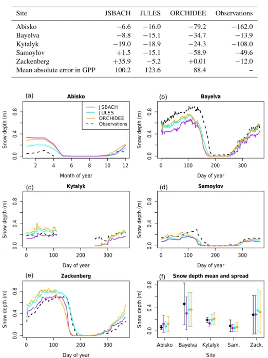
The seasonal cycle of snow depth is shown in Fig. 1. It de-pends strongly on the snowfall driving data. Since the snow-fall was back-calculated from the snow depth, the accumu-lation period should match well with observations. There is still some variation due to the fresh snow density in the mod-els (which can differ from both the assumed density in mak-ing the drivmak-ing data and between the models), and further-more the compaction of the snow is dependent on the model process representation and physical conditions. Nonetheless, for the most part the models make a reasonable simulation of the snowpack accumulation and compaction, with the excep-tion of Abisko, where the models are all biased high. Here, snow inputs are particularly uncertain as no high-resolution time series of snow depth are available (unlike the other sites). We performed a sensitivity study to test the impact of uncertainties or variability in snow depth on the simulated carbon cycle processes. In this study, a reduction of 50 % in snowfall allows the models to simulate a realistic snow depth at Abisko – see the Supplement. The impacts on soil carbon stocks and fluxes are fairly small, however (between 0.2 and 10 %; Figs. S7 and S8).
During the melting season the models are less accurate than during accumulation, with the snow often melting too early, by up to 25 days in the most extreme case. Our method of back-calculating snowfall from snow depth may miss some snowfall events during the melt season. There are also many other potential influences such as albedo effects, snow– vegetation interactions and the influence of wind-blown sed-iment. For example, the vegetation in the models is quite
Table 1. Key features of the land surface models used in this study.
Process JSBACH JULES ORCHIDEE
PFTs 20 9 (+4 crop/pasture) 13
PFT that grows/is used Tundra C3 grass C3 grass
Dynamic vegetation No Yes No
Dynamic phenology Yes Yes Yes
Nutrient limitation No No No
Soil carbon One layer Multilayer Multilayer
Soil carbon mixing No Yes Yes
Deep soil respiration None Suppressed Not suppressed
Soil latent heat Yes Yes Yes
Snow Multilayer Multilayer Multilayer
Table 2. Key climatic and physical variables at the sites.
Abisko Bayelva Kytalyk Samoylov Zackenberg
Latitude 68.35 78.92 70.83 72.22 74.5
Longitude 19.05 11.93 147.5 126.28 −20.6
Elevation 385 m a.s.l. 25 m a.s.l. 10 m a.s.l. 6 m a.s.l. 40 m a.s.l.
Mean annual air temp. −0.6◦C −5◦C −10.5◦C −12.5◦C −9◦C
Max. monthly air temp. 11◦C 5◦C 10◦C 10◦C 6.5◦C
Min. monthly air temp. −11◦C −13◦C −34◦C −33◦C −20◦C
Annual precipitation 350 mm 400 mm 230 mm ∼190 mm 260 mm
Fraction as snow ∼40 % ∼75 % ∼50 % ∼30 % ∼85 %
Typical snow depth 0.1 m 0.5–0.8 m 0.2–0.4 m 0.2–0.4 m 0.1–1.3 m
Active-layer depth 0.55–1.2 m 1–2 m 0.25–0.5 m <1 m 0.45–0.8 m
Permafrost temperature ∼0◦C −2 to −3◦C −8◦C −10◦C −6.5 to −7◦C
Soil type (mineral/organic) Organic Mineral Organic Organic Mineral
tall (up to 1 m) and can lead to a lower albedo in the models than reality, and thus faster snowmelt (this is mod-elled by interpolating between snow-covered and snow-free albedo depending on snow depth and vegetation height). At Bayelva, where the vegetation is particularly small (∼ 5 cm), there is a notable underestimation of the snow depth and early snowmelt in all models, which supports this hypoth-esis (snow at Bayelva can be modelled very well when veg-etation is not included; López-Moreno et al., 2016). Snow-drift is only represented by scaling the snowfall data to match the observed snow accumulation, which limits the extent to which snowpack dynamics can be recreated by the models.
It is important to be careful when modelling snow depth based on single-point observations, as they may not be resentative of the area as a whole. Further details on the rep-resentativity of snow depths are given in the Supplement. The sensitivity of carbon cycle processes to increased or reduced snowfall is discussed in Sect. 3.5 and 3.6.1.
3.2 Soil temperature
Soil temperature annual cycles at ∼ 40 cm depth are shown in Fig. 2. In general the models simulate the soil temperature at mineral soil sites quite well: see the Bayelva and Zackenberg
sites in Fig. 2. There are greater errors in the simulation of organic soils: Abisko, Kytalyk and Samoylov in Fig. 2.
For JSBACH and ORCHIDEE, the annual cycles of tem-perature are too large for the organic sites, indicating that these models need to better represent the insulating and damping properties of organic soils. To illustrate this, addi-tional observations from mineral soil at the nearby research station (where there is no permafrost) are shown on the Abisko plot (Fig. 2). This line matches much more closely with the ORCHIDEE and JSBACH simulations, suggesting that these models are behaving thermally like a mineral soil. At Abisko, permafrost only occurs in peat plateaus, and thus including organic soil properties in the models is essential for capturing the difference between permafrost and non-permafrost conditions.
In JULES, however, the annual cycle amplitude is too small at the organic sites and also at Zackenberg, mostly due to biases in the winter soil temperatures. This suggests that the snow thermal conductivity or density may be too low in JULES. A similar problem was found with a previous JULES simulation of Samoylov island, using a similar model set-up and forcing data (Chadburn et al., 2015a). There, the winter soil temperature was improved by increasing snow density. Indeed, the conductivity of snow in the JULES simulations
Table 3. Mean NEE budget (g C m−2yr−1), showing that in general this is smaller than the errors in simulated GPP; therefore, the noise is larger than the signal in this data. Positive numbers represent a carbon source.
Site JSBACH JULES ORCHIDEE Observations
Abisko −6.6 −16.0 −79.2 −162.0
Bayelva −8.8 −15.1 −34.7 −13.9
Kytalyk −19.0 −18.9 −24.3 −108.0
Samoylov +1.5 −15.1 −58.9 −49.6
Zackenberg +35.9 −5.2 +0.01 −12.0
Mean absolute error in GPP 100.2 123.6 88.4 –
2 4 6 8 10 12 0.0 0.4 0.8 Abisko Month of year Sno w depth (m) JSBACH JULES ORCHIDEE Observations 0 100 200 300 0.0 0.4 0.8 Bayelva Day of year Sno w depth (m) 0 100 200 300 0.0 0.4 0.8 Kytalyk Day of year Sno w depth (m) 0 100 200 300 0.0 0.4 0.8 Samoylov Day of year Sno w depth (m) 0 100 200 300 0.0 0.4 0.8 Zackenberg Day of year Sno w depth (m) 0.0 0.4 0.8
Snow depth mean and spread
Site
Sno
w depth (m)
Abisko Bayelva Kytalyk Sam. Zack.
● ● ● ● ● ● ● ● ● ● ● ● ● ● ● ● ● ● ● ● (a) (b) (c) (d) (e) (f)
Figure 1. Mean annual cycle of snow depth at each site, showing both observations and models. In panel (f), Samoylov and Zackenberg are abbreviated to “Sam.” and “Zack.”. Mean annual cycle is calculated from a single site over a number of years, except for Abisko, where measurements were taken at several different locations in the mire. See Table S1 for the years used at each site.
is between 0.03 and 0.1 Wm−1K−1 at the sites with shal-low snow (and in the upper layers of the snowpack at sites with deeper snow), which is considerably lower than typ-ical values for similar tundra sites, which are around 0.2– 0.3 Wm−1K−1, at least for the upper part of the snowpack (Gouttevin et al., 2012b; Domine et al., 2016). See the Sup-plement for further discussion on snow conductivity and den-sity.
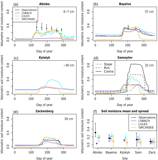
3.3 Soil moisture
As with temperature, the (unfrozen) soil moisture is simu-lated well at mineral soil sites – see Bayelva and Zackenberg in Fig. 3. In the winter, ORCHIDEE does not represent the unfrozen water fraction in frozen soils, but the other models simulate a reasonable water content in winter. However, soil moisture is in general too low at organic sites - Samoylov and Abisko mire. The soils should be able to hold water near
0 100 200 300 −20 −10 0 10 Abisko Day of year Temper ature ( ° C) 50cm Observations JSBACH JULES ORCHIDEE Mineral site (no PF)
0 100 200 300 −20 −10 0 10 Bayelva Day of year Temper ature ( ° C) 40cm 0 100 200 300 −20 −10 0 10 Kytalyk Day of year Temper ature ( ° C) 25cm 0 100 200 300 −20 −10 0 10 Samoylov Day of year Temper ature ( ° C) 42cm 0 100 200 300 −20 −10 0 10 Zackenberg Day of year Temper ature ( ° C) 40cm −20 −10 0 10
Soil temperature mean and spread
Site
Temper
ature (
°
C)
Abisko Bayelva Kytalyk Sam. Zack.
● ● ● ● ● ● ● ● ● ● ● ● ● ● ● ● ● ● ● ● (a) (b) (c) (d) (e) (f)
Figure 2. Mean annual cycle of soil temperature at each site, showing both observations and models. Depths of observations: Abisko: 50 cm; Bayelva: 40 cm; Kytalyk: 25 cm; Samoylov: 42 cm; Zackenberg: 40 cm. JULES and ORCHIDEE take the nearest soil layer and JSBACH is interpolated to the correct depth, as soil layers are not resolved well enough to get close to the right depth. In panel (f), Samoylov and Zackenberg are abbreviated to “Sam.” and “Zack.”. See Table S1 for the years used at each site.
the surface and remain saturated very close to the surface (or even above). This points to problems with the hydrology schemes. The soil moisture is very important for the soil tem-peratures, and it can also have a strong influence on soil car-bon stocks and the partitioning of decomposition into CO2 and methane. Furthermore, it influences vegetation growth, and thus the uptake of CO2from the atmosphere. Therefore, it is important to further improve the soil hydrology in these models.
Note that saturated zones can be influenced by landscape heterogeneity and lateral water fluxes that would not be cap-tured in a point simulation. This can potentially be simulated by the models as a landscape average (see, for example, Ged-ney and Cox, 2003). However, such schemes simulate only a grid-box-mean water content, which does not capture, for example, the influence of anaerobic conditions on decompo-sition.
Figure 3 shows quite a large variation in the timing of freeze-up and thaw between the models, reflecting the
soil temperature differences in Fig. 2. Correspondingly, the largest differences are at the organic soil sites.
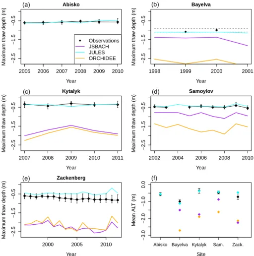
3.4 ALT
The active-layer depth is shown in Fig. 4. In the models it is calculated with interpolation of soil temperatures to find the daily thaw depth, except in JULES, which uses the method of (Chadburn et al., 2015a). The two methods differ at most within the thickness of the soil layers; see Table A2. In OR-CHIDEE and JSBACH the active layer is too deep, which corresponds to the too-warm soil temperatures in summer (Fig. 2). In JSBACH the summer temperatures are only a little warmer than the observations – certainly closer than in ORCHIDEE, yet at some sites the active layer is just as deep. This is because technically the ALT (active layer thickness) cannot be diagnosed correctly in JSBACH, given the thick soil layers below 20 cm depth (see Table A2). Increasing the resolution of the soil layers, while it does not make a big dif-ference to the soil temperature profile, has a very large
im-0 100 200 300 0.0 0.4 0.8 Abisko Day of year Volumetr
ic soil moisture content
0−7cm Observations JSBACH JULES ORCHIDEE 0 100 200 300 0.0 0.4 0.8 Bayelva Day of year Volumetr
ic soil moisture content
37cm 0 100 200 300 0.0 0.4 0.8 Kytalyk Day of year Volumetr
ic soil moisture content
~30cm 0 100 200 300 0.0 0.4 0.8 Samoylov Day of year Volumetr
ic soil moisture content
32cm Slope Rim Centre 0 100 200 300 0.0 0.4 0.8 Zackenberg Day of year Volumetr
ic soil moisture content
30cm
0.0
0.2
0.4
0.6
Soil moisture mean and spread
Site
Volumetr
ic soil moisture content
Abisko Bayelva Kytalyk Sam. Zack.
● ● ● ● ● ● ● ● ● ● ● ● ● ● ● ● ● ● ● Observations JSBACH JULES ORCHIDEE (a) (b) (c) (d) (e) (f)
Figure 3. Mean annual cycle of unfrozen soil moisture at each site, showing both observations (where available) and models. Depths are as follows: JSBACH: 19 cm for all sites (this is the closest to 30 cm – the next layer is at 78 cm), except Abisko, which is 3 cm. JULES: 32 cm (except Abisko, which is 3 cm). ORCHIDEE: 36 cm (except Abisko, which is 4 cm). Observations: Bayelva: 37 cm; Samoylov: 32 cm; Zackenberg: 30 cm; Abisko: 0–7 cm. For Samoylov, three different soil moisture profiles are shown that represent different parts of the polygonal microtopography. In panel (f), Samoylov and Zackenberg are abbreviated to “Sam.” and “Zack.”. See Supplement Table S1 for the years used at each site.
pact on the simulation of the active-layer depth, as shown by (Chadburn et al., 2015b). In JULES there is generally quite a good match to the observations as supported by the fact that the summer soil temperatures match closely with the obser-vations for most sites. For Zackenberg the active layer is a little too shallow, but still in the range of observed values. This shows the importance of both resolving the soil column and the insulating effects of organic matter for determining the summer soil temperatures (Dyrness, 1982).
3.5 Soil carbon stocks
JULES and ORCHIDEE represent a vertical profile of soil carbon, whereas JSBACH does not. Without a vertical rep-resentation of soil carbon it is not possible to simulate per-mafrost carbon stocks because all of the carbon is subject to the seasonal freezing and thawing of the active layer and the model does not contain any inert, permanently frozen carbon.
Therefore, a vertical representation of soil carbon is prerequi-site for simulating soil carbon stocks at these prerequi-sites. However, JULES and ORCHIDEE have some problems in simulating the profiles – Fig. 5. The most obvious problem is underesti-mation: there is much too little carbon simulated at many of the sites (see the last panel in Fig. 5, showing total column soil carbon). For the sites at which the quantity of soil car-bon is somewhat realistic, the shape of the profiles vary from a steep exponential-looking decay with depth to a shallower decline with more carbon in the deeper soil. The same kind of profiles are seen in the observations, particularly for the mineral soil sites (Bayelva and Zackenberg). However, nei-ther of the models can produce the carbon-rich peaty layers of the organic soils. To simulate this would require additional process representation in the models, including representing saturated (and thus anaerobic) conditions in peat soil, and a dynamic representation of bulk density.
2005 2006 2007 2008 2009 2010 −2.5 −1.5 −0.5 Abisko Year Maxim um tha w depth (m) ● ● ● ● ● ● Observations JSBACH JULES ORCHIDEE −2.5 −1.5 −0.5 Bayelva Year Maxim um tha w depth (m) 1998 1999 2000 2001 2007 2008 2009 2010 2011 −2.5 −1.5 −0.5 Kytalyk Year Maxim um tha w depth (m) ● ● ● ● ● 2002 2004 2006 2008 2010 −2.5 −1.5 −0.5 Samoylov Year Maxim um tha w depth (m) ● ● ● ● ● ● ● ● 2000 2005 2010 −2.5 −1.5 −0.5 Zackenberg Year Maxim um tha w depth (m) ● ● ● ● ● ● ● ● ● ● ● ● ● ● ● ● ● −3.0 −2.0 −1.0 0.0 Site Mean AL T (m) ● ● ● ● ●
Abisko Bayelva Kytalyk Sam. Zack.
(a) (b)
(c) (d)
(e) (f)
Figure 4. Maximum summer thaw depth (active layer) over a number of years at each site, comparing observations and models. Dotted lines in panel (b) represent the range of observed estimates. For all other panels, CALM grids are used, and the error bars show the full range of measured values in the grid. In panel (f) the error bars show the mean of the upper and lower limits from the previous panels.
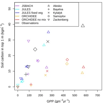
The reasons for the major underestimation are different in JULES and ORCHIDEE. In JULES, the main problem is that the GPP is underestimated; therefore, there are not enough plant inputs to accumulate carbon in the soil. This is made clearer by Fig. 6, which shows the relationship between GPP and the top 1 m soil carbon stocks. In JULES, the relation-ships are very similar to the observations, which indicates that the turnover of carbon in the soil is reasonable in JULES. Therefore, if the GPP were large enough, the soil carbon stocks would be much more realistic. In ORCHIDEE, the story is different. Even when the vegetation is productive, the soil carbon stocks are still very low. This indicates a problem with the soil carbon decomposition. There are two factors that could affect this. Firstly, the soil temperatures in OR-CHIDEE are much too warm, and the active layer is too deep (Figs. 2 and 4). This can lead to too much decomposition. In order to improve this, the model needs to better represent the insulation from the organic soils. Another possible problem is the deep soil respiration. In ORCHIDEE the only factor that suppresses the soil respiration at depth is the cold and/or
frozen nature of the ground. In JULES, however, there is an additional decay of respiration with depth that empirically represents some processes that are missing in the model (fol-lowing the implementation in the Community Land Model; see Koven et al., 2013). Including this in ORCHIDEE could lead to a higher carbon stock at depth. The deeper soil car-bon stocks are also influenced by long-term burial processes, which are only represented by a simple diffusion scheme in these models. We include JSBACH in Fig. 6 because the top 1 m of soil carbon is mostly in the active layer. Given that the decomposition in JSBACH is controlled by the temperature of the top soil layer (3 cm), it is not surprising that the re-lationships are not captured perfectly, as the upper soil layer will be much more sensitive to variations in temperature than the deeper ones. However, on average the turnover is quite realistic for this model.
It should be noted that the observed relationship in Fig. 6 may be confounded by the history of soil carbon formation at these sites. There is inconsistency between Holocene climate and the pre-industrial climate used in model spin-ups.
Re-0 20 40 60 80 −3.0 −2.0 −1.0 0.0 Abisko (1)
Soil carbon density (kgm−3)
Depth (m) 0 20 40 60 80 −3.0 −2.0 −1.0 0.0 Bayelva (2)
Soil carbon density (kgm−3)
Depth (m) 0 20 40 60 80 −3.0 −2.0 −1.0 0.0 Kytalyk (3)
Soil carbon density (kgm−3)
Depth (m) Observations
JULES JULES fixed veg ORCHIDEE ORCHIDEE no mix 0 20 40 60 80 −3.0 −2.0 −1.0 0.0 Samoylov (4)
Soil carbon density (kgm−3)
Depth (m) 0 20 40 60 80 −3.0 −2.0 −1.0 0.0 Zackenberg (5)
Soil carbon density (kgm−3)
Depth (m) 1 2 3 4 5 0 20 40 60 80 100
Total column soil carbon
Site no. Soil carbon (kgm − 2 ) Total column Top 1m
Figure 5. Profile of soil carbon at each site (kg m−3). Observations and two of the models (ORCHIDEE and JULES) are shown, as these models have a vertically resolved soil carbon profile. Dotted and solid lines in the second panel (Bayelva) show two different land cover types in the vicinity of the site (solid: barren ground; dotted: sparse shrub–moss tundra.) Note that site numbers in the last panel are given in the headings of the preceding panels.
constructed Holocene climate for the Northern Hemisphere is warmer than pre-industrial (Marcott et al., 2013), and pos-sibly wetter, favouring the formation of peat; thus, some un-derestimation by the models may be expected.
The soil carbon stocks are sensitive to changes in snow depth in these models (see Fig. S8), through changes in soil temperature (JSBACH) and changes in vegetation growth (JULES). In JULES, both vegetation and soil temperature changes affect the soil carbon, but the vegetation effect dom-inates. In fact, for two of the sites (Kytalyk and Samoylov), the vegetation coverage is so different during spin-up that the simulation with increased snowfall accumulates twice as much soil carbon as the default case (although the stocks are still much too small and the absolute difference is less than 10 kg m−2in the whole soil column).
We conclude that improving soil carbon stocks demands a different priority in each model. For JULES, the first pri-ority is to simulate realistic vegetation productivity, for OR-CHIDEE it is to improve the soil carbon decomposition and for JSBACH it is to represent a vertical profile of soil car-bon. Assuming we can combine the best features from all of the models, the greatest difference between the observed and simulated profiles will be the peaty, organic layers that are
present in observations and not models (Fig. 5). Therefore, the next priority for model development is to better represent these organic soils. See Frolking et al. (2010) and Schuldt et al. (2013) for examples of modelling peat. While peatlands represent a small fraction of the land surface, they contain very large carbon stocks (Yu et al., 2010); thus, it is impor-tant to include them in ESMs.
3.6 Carbon fluxes
Figure 7 shows the seasonal cycle of CO2flux at every site. The daytime and night-time fluxes are plotted separately (partitioned by incoming shortwave radiation), showing in general uptake during the day and emissions during the night. For the most part, the models show uptake and emissions at the same time as the observations and a similar timing of peak uptake and emission (one exception being the spring daytime flux in ORCHIDEE; see Sect. 3.6.1).
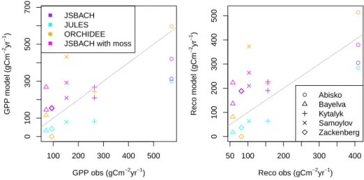
From the observations we also have the gap-filled esti-mates of annual GPP and Reco, which are compared with the annual totals for each model in Fig. 8 (the moss GPP shown here is discussed in Sect. 3.6.3). For the GPP we see that for each model there is a positive correlation (sites with
0 100 200 300 400 500 600 700 0 10 20 30 40 50 GPP (gm−2yr−1) −
Soil carbon in top 1
m (kgm
2)
JSBACH JULES JULES fixed veg ORCHIDEE ORCHIDEE no mix Observations Abisko Bayelva Kytalyk Samoylov Zackenberg
Figure 6. GPP compared with the top 1 m soil carbon at each site. The top 1 m soil carbon values are for the tower footprint area (see Table S2), so that equivalent values are being compared.
larger GPP in reality have larger GPP in the models), but that the overall values are too small for JULES, for ORCHIDEE there is a bigger variation, and for JSBACH they tend to be too large for the less productive sites and too small for the more productive sites – i.e. the slope of the relationship be-tween model and observations is too shallow. Nonetheless, a significant amount of the variation between sites is captured by the models, to which the only inputs are climate data and soil properties. Of these, climate is the main driver of vege-tation growth in these models (since nutrient limivege-tation is not included, the soil only impacts the vegetation through mois-ture stress – which is also partly climate-related). Therefore, we can say that a lot of the difference between the GPP and Reco across different sites is due to the difference in climate. In fact, in JULES and JSBACH, over 90 % of the variation in GPP between sites is explained by the model, despite the systematic biases (R squared values of modelled GPP against observed GPP: JSBACH – 0.94; JULES – 0.95; ORCHIDEE – 0.63). This suggests that a model based on climate alone and with one tundra PFT could capture most of the variabil-ity in tundra carbon uptake, if the vegetation was correctly calibrated. This is a promising sign that the model simula-tions could be easily improved.
Due to the magnitude of errors in GPP and Reco, when considering the difference between the two – the NEE – the noise will be larger than the signal. Nonetheless, the mod-els and observations both generally show a carbon sink in the present day due to environmental conditions being more
favourable for growth (warmer, more CO2) than in the pre-industrial spin-up period (Table 3).
3.6.1 Drivers of carbon fluxes
The models indicate different drivers of GPP in different parts of the growing season. In particular, the increase in GPP in the first half of the season is driven by increasing LAI, and the downward trend in GPP in the second half of the season is driven by shortwave radiation. There is also a tempera-ture dependence in all parts of the growing season. These relationships are shown in Fig. S1. Figure S1 also shows the plant respiration in the models, which exhibits a simi-lar behaviour to the GPP, being influenced by temperature, shortwave radiation and LAI. The fact that these variables influence the GPP and autotrophic respiration is clear from the model structure (for example Knorr, 2000; Clark et al., 2011); however, the apparent split between the two halves of the season is an emergent behaviour.
The other component of the Reco is heterotrophic respi-ration. This does not exhibit the same dependencies as the plant respiration as it is determined by below-ground condi-tions. The heterotrophic respiration has a loose relationship with air temperature and a much stronger relationship with the ∼ 20 cm soil temperature – see Supplement Fig. S2.
In order to compare the photosynthesis schemes in the models more directly, we normalise by the LAI. It then be-comes clear that the photosynthesis models in JSBACH and ORCHIDEE are in fact quite similar. Figure 9 shows the nor-malised GPP (per square metre of leaf) plotted against the air temperature and shortwave radiation. JSBACH and OR-CHIDEE show similar relationships, although OROR-CHIDEE still has a slightly higher GPP, potentially explained by the fact that the Vc,max is higher. In these plots we also show the limited data that we can plot from observations using MODIS LAI. It is clear that the normalised GPP in JULES is too low (this is a problem, probably related to canopy scal-ing, that requires attention in the model), but for JSBACH and ORCHIDEE the GPP is approximately consistent with the observations. The observations are a little higher than the models, but this is largely influenced by underestimated LAI at Samoylov (note that for the other sites, MODIS LAI com-pares reasonably with ground-based estimates). Moss cover is close to 100 % at Samoylov (Kutzbach et al., 2007) and, by contrast, maximum LAI from MODIS is only around 0.3. This could be due to the large size of the MODIS pixels (1 km × 1 km) leading to the inclusion of water in the pixel, or because the moss has a different absorption spectrum from vascular plants and could register as bare soil. Whatever the cause, the GPP per unit LAI at Samoylov would be at least doubled by this underestimation of LAI, and if we were to account for this, the observation-based estimates would be very close to the JSBACH and ORCHIDEE results.
Aside from JULES being biased low, we therefore con-clude that the main source of error in the modelled seasonal
0 100 200 300 −1 0 1 2 3 4 5 Abisko night Day of year NEE ( µmol m −2s −1) 0 100 200 300 −8 −6 −4 −2 0 2 Abisko day Day of year NEE ( µmol m −2s −1) Observations JSBACH JULES ORCHIDEE 0 100 200 300 −1 0 1 2 3 4 5 Bayelva night Day of year NEE ( µmol m −2s −1) 0 100 200 300 −8 −6 −4 −2 0 2 Bayelva day Day of year NEE ( µmol m −2s −1) 0 100 200 300 −1 0 1 2 3 4 5 Kytalyk night Day of year NEE ( µmol m −2s −1) 0 100 200 300 −8 −6 −4 −2 0 2 Kytalyk day Day of year NEE ( µmol m −2s −1) 0 100 200 300 −1 0 1 2 3 4 5 Samoylov night Day of year NEE ( µmol m −2s −1) 0 100 200 300 −8 −6 −4 −2 0 2 Samoylov day Day of year NEE ( µmol m −2s −1) 0 100 200 300 −1 0 1 2 3 4 5 Zackenberg night Day of year NEE ( µmol m −2s −1) 0 100 200 300 −8 −6 −4 −2 0 2 Zackenberg day Day of year NEE ( µmol m −2s −1)
Figure 7. Mean annual cycles of CO2fluxes for all sites, observations and models. Left: night-time flux; right: daytime flux (corresponding to incoming shortwave radiation > 20 Wm−2). See Table S1 for the years used at each site.
● 100 200 300 400 500 0 100 300 500 700 GPP obs (gCm−2yr−1) GPP model (gC m − 2y r − 1) ● ● ● JSBACH JULES ORCHIDEE JSBACH with moss
● 50 100 200 300 400 0 100 200 300 400 500 Reco obs (gCm−2yr−1) Reco model (gC m − 2 y r − 1 ) ● ● ● ● Abisko Bayelva Kytalyk Samoylov Zackenberg
Figure 8. Mean annual GPP (gross primary productivity) and Reco (ecosystem respiration) from the models, plotted against the observation-derived values for the same time periods. See Table S1 for the years used at each site.
−5 0 5 10 0 2 4 6 8 Air temperature (°C) G P P p e r u n it le a f a re a ( µ m o l m s ) − 2 − 1 ● ●● ●● ●● ●●●●●●●●●●●● ●●●● ●●●● ● ●● ●●● ● ●●●●●●● ● ●●●●●●● ●●●●● ●●● ● ●●●●●● ●●●●●● ● ● ●●●●●●●●●●●●●●●●●●● ● ●●●●●●● ● ●●●●●● ●●●●●●● ●●●● ● ●● ● ●●●●●●● ● ●●●●●●● ●●●●● ●●● ● ●●●●●● ●●●●●● ● ● ●●●●●●●●●●●●●●●●●●● ● ●●●●●●● ● ●●●●●● ●●●●●●● ●●●● ● ●● ● ●●●● ●●●●●●● ●● ●●● ● ●●●●●●●●●● ●●● ● ●●●●● ●●●● ● ● ●●●●●●●● ● ●●●● ● ●●●●● ●●●●●●● ●●●● ● ●● ● ● ● ●●●● ●●● ● ●● ●●●●●● ●●●● ●●●●●●●●●●● ●● ● ●●●●●● ●● ●● ●●●●●●●●●● ● ●● ●●●●●●● ●●●● ●●●●●●●●● ●●●●●●●●● ● ●● ●●●●● ●● ●●●●●●●●●●●●●●●●● ●● ●●●●● ● ●●●●●● ●● ●● ●●●●●●●●●● ● ●● ●●●●●●● ●●●● ●●●●●●●●● ●●●●●●●●● ● ●● ●●●●● ●● ●●●●●●●●●●●●●●●●● ●● ●●●●● ● ●●●●●●● ● ●●●●●●● ●●●●●● ● ●●●●●● ● ● ● ● ● ● ● ● ● ● ● ● ● ● Models Jan–Mar Apr–May Jun–Jul Aug–Sep Oct−Dec 0 50 100 150 200 250 300 350 0 2 4 6 8
Incoming shortwave radiation (Wm )−2
GPP per unit leaf area (
µ mol m − 2 s − 1 ) ● ● ● ● ● ● ● ● ● ● ● ● ● ● ● ● ●●●●●●●●●●●●●●●●●●●●●●●●●●●●●●●●●●●●●●● ●● ●●●●● ●● ●●●●●●● ●●●●●● ●● ●●●●● ●●●●●● ● ● ● ● ● ● ● ● ● ● ● ● ● ● ● ● ●●●●●●●●●●●●●●●●●●●●●●●●●●●●●●●●●●●●●●● ●● ●●●●● ●● ●●●●●●● ●●●●●● ●● ●●●●● ●●●●●● ● ● ● ● ● ● ● ● ● ● ● ● ● ● ● ● ●●●●●●●●●●●●●●●●●●●●●●●●●●●●●●●●●●●●●●● ●● ●●●●● ●● ●●●●●●● ●●●●●● ●● ●●●●● ●●●●●● ● ● ● ● ● ● ● ● ● ● ● ● ● ● ● ● ● ● ● ● ● ● ● ● ● ● ● ● ● ● ● ● ● ● ● ● ● ● ● ● ● ● ● ● ● ● ● ●●●●●●●●●●●●●●●●●●●●●●●●●●●●●●●●●●●●●●●●●●● ● ● ● ● ● ● ● ● ● ● ● ● ● ● ● ● ● ● ● ● ● ● ● ● ● ● ● ● ● ● ● ● ● ● ● ● ● ● ● ● ● ● ● ● ● ● ● ●●●●●●●●●●●●●●●●●●●●●●●●●●●●●●●●●●●●●●●●●●● ● ● ● ● ● ● ● ● ● ● ● ● ● ● ● ● ● ● ● ● ● ● ● ● ● ● ● ● ● ● ● ● ● ● ● ● ● ● ● ● ● ● ● ● ● ● ● ●●●●●●●●●●●●●●●●●●●●●●●●●●●●●●●●●●●●●●●●●●● ● ● ● ● ● ● ● ● ● ● ● ● ● ● ● ● ● ● ● ● ● ● ● ● ● ● ● ● ●● ●●●●●●●●●●●●●●●●●●●●●●●●●●●●●●●●●●●●●●●●●●●●●●●●●●●●● ● ● ● ●●●● ● ● ● ● ● ● ● ● ● ● ● ● ● ● ● ● ● ● ● ● ● ● ● ● ● ● ● ● ●● ●●●●●●●●●●●●●●●●●●●●●●●●●●●●●●●●●●●●●●●●●●●●●●●●●●●●● ● ● ● ●●●● ● ● ● ● ● ● ● ● ● ● ● ● ● ● ● ● ● ● ● ● ● ● ● ● ● ● ● ● ●● ●●●●●●●●●●●●●●●●●●●●●●●●●●●●●●●●●●●●●●●●●●●●●●●●●●●●● ● ● ● ●●●● ● ● ● ● ● ● ● ● ● ● ● ● ● ● ● ● ● ● ● ● ● ● ● ● ● ● ● ● ● ●●●●●●●●●●●●●●●●●●●●●●●●●●●●●●●●●●●●●●●●●●●● ●● ●●●●●●●● ●●●●●●● ● ● ● ● ● ● ● ● ● ● ● ● ● ● ● ● ● ● ● ● ● ● ● ● ● ● ● ● ● ●●●●●●●●●●●●●●●●●●●●●●●●●●●●●●●●●●●●●●●●●●●● ●● ●●●●●●●● ●●●●●●● ● ● ● ● ● ● ● ● ● ● ● ● ● ● ● ● ● ● ● ● ● ● ● ● ● ● ● ● ● ●●●●●●●●●●●●●●●●●●●●●●●●●●●●●●●●●●●●●●●●●●●● ●● ●●●●●●●● ●●●●●●● ● ● ● ● ● ● ● ● ● ● ● ● ● ● ● ● ● ● ● ● ● ● ● ● ● ● ● ● ● ● ● ● ● ● ● ● ●●●●●●●●●●●●●●●●●●●●●●●●●●●●●● ●●● ●●●●●●●●●● ●●● ●●● ●●●●● ● ● ● ● ● ● ● ● ● ● ● ● ● ● ● ● ● ● ● ● ● ● ● ● ● ● ● ● ● ● ● ● ● ● ● ● ●●●●●●●●●●●●●●●●●●●●●●●●●●●●●● ●●● ●●●●●●●●●● ●●● ●●● ●●●●● ● ● ● ● ● ● ● ● ● ● ● ● ● ● ● ● ● ● ● ● ● ● ● ● ● ● ● ● ● ● ● ● ● ● ● ● ●●●●●●●●●●●●●●●●●●●●●●●●●●●●●● ●●● ●●●●●●●●●● ●●● ●●● ●●●●● ● ● ● ● ● ● ● ● ● ● ● ● ● ● ● ● ● ● ● JSBACH JULES ORCHIDEE Observations
Figure 9. Relationship of normalised GPP (GPP per square metre of leaf) to air temperature and incoming solar radiation. All models and sites are shown, plus observationally derived values using GPP estimated from eddy covariance data and LAI from MODIS (MODIS15A2, 2016); see Sect. 2.1.8.
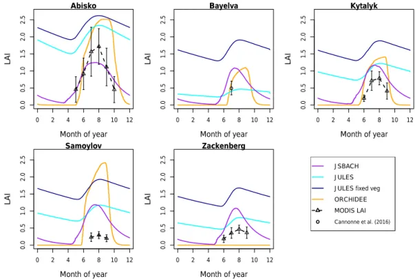
cycle of GPP is the huge variation in the simulated LAI. This is shown in Fig. 10. For example, ORCHIDEE LAI remains at zero in the early season, when the observations and other models show carbon uptake, and it suddenly increases to a very large value later in the season, then showing an uptake that is much larger than the observations (Fig. 7). In fact, at Zackenberg the cumulative temperature is never high enough to initiate budburst in the model; thus, the LAI is always zero. These problems lead to unrealistic daytime emissions dur-ing sprdur-ing from ORCHIDEE in Fig. 7 for most sites, and no fluxes at all for Zackenberg. Since the GPP seems to be con-sistent with observations when the impact of LAI is removed, we conclude that if the models could simulate the correct LAI they would largely simulate the correct GPP. JULES captures more of the difference in LAI between the sites than the
other models (and subsequently captures more of the inter-site variation in GPP). This is because JULES is running a dynamic vegetation scheme that allows the vegetation frac-tion to vary. The LAI from JULES with fixed vegetafrac-tion is also shown in Fig. 10 and captures less of the inter-site vari-ability. Therefore, both improving the LAI and including a dynamic vegetation scheme is the priority for improved sim-ulations of tundra carbon uptake.
Carbon fluxes are also sensitive to soil moisture, as seen in simulations with increased or decreased snowfall, in which differences in soil moisture availability in summer are re-flected by changes in annual mean GPP, Reco and vegeta-tion fracvegeta-tion in JULES (Fig. S7), in line with (Frost and Ep-stein, 2014). Therefore, realistic simulation of precipitation