How Adsorption of Pheromones on Aerosols Controls Their Transport

HAL Id: hal-02924943

https://hal.umontpellier.fr/hal-02924943

HAL is a multi-disciplinary open access

archive for the deposit and dissemination of sci-entific research documents, whether they are pub-lished or not. The documents may come from teaching and research institutions in France or abroad, or from public or private research centers.

L’archive ouverte pluridisciplinaire HAL, est destinée au dépôt et à la diffusion de documents scientifiques de niveau recherche, publiés ou non, émanant des établissements d’enseignement et de recherche français ou étrangers, des laboratoires publics ou privés.

How Adsorption of Pheromones on Aerosols Controls

Their Transport

Ludovic Jami, Thomas Zemb, Jérôme Casas, Jean-François Dufrêche

To cite this version:

Ludovic Jami, Thomas Zemb, Jérôme Casas, Jean-François Dufrêche. How Adsorption of Pheromones on Aerosols Controls Their Transport. ACS Central Science, ACS Publications, 2020, 6 (9), pp.1628-1638. �10.1021/acscentsci.0c00892�. �hal-02924943�

How Adsorption of Pheromones on Aerosols Controls Their

Transport

Ludovic Jami, Thomas Zemb, Jérôme Casas, and Jean-François Dufrêche

*

Cite This:ACS Cent. Sci. 2020, 6, 1628−1638 Read Online

ACCESS

*

pheromone molecules in an atmosphere containing aerosols. Many pheromones are hydrophobic molecules containing polar groups. They are low volatile and have some properties similar to those of hydrotropes. They therefore form a nonsolublefilm at the water−air interface of aerosols. The fate of a small pheromone puff in air is computed through reaction-diffusion equations. Partitioning of pheromones between the gas and the aerosol surface over time is studied for various climate conditions (available aerosol surface) and adsorption affinities (energy of adsorption). We show that, for adsorption energy above 30 kBT per molecule, transport of

pheromones on aerosols dominates over molecular transport typically 10 s after pheromone emission, even when few adsorbing

aerosols are present. This new communication path for airborne chemicals leads to distinctive features including enhanced signal sensibility and increased persistence of pheromone concentration in the air due to slow diffusion of aerosols. Each aerosol droplet has the ability to adsorb thousands of pheromones to the surface, keeping a“history” of the atmospheric content between emission and reception. This new mechanism of pheromone transport leads to dramatic consequences on insect sensing revisiting the way we figure the capture of chemical signals.

■

Chemical communication through sex pheromones is critical for insect life, enabling mate finding for reproduction. Communication with sex pheromones requires persistence of the olfactory signal in the air to recruit males far from the source. After release, pheromones are thought to be dispersed as gas molecules.1−3

Nevertheless, many pheromones, regarding their chemical structure, are typical low-volatile organic molecule of molar mass 200−400 combining rigidity of some parts, hydrocarbon chains, very apolar sites, polarizability with aromatic rings, as well as polar groups such as OH. Unlike lipids, they have good solubility in apolar solvents. Unlike detergents and surfactant molecules, pheromones are not soluble in water. They are close to neutral hydrotropes that are soluble in water and in solvo-surfactants,4−6 except for water solubility. They have therefore a high affinity for the water−air interface, forming an insoluble monolayerfilm with an area per site of typically less than 1 nm2molecule−1.

One good example is given by bombykol, from the moth Bombyx mori which is a model species for chemical communication.7 It is composed of a 16C-long carbon chain and an alcohol headgroup. Its boiling point is predicted to be 298 °C, and its saturation pressure is 7.5 Pa.8 Thus, it is a typically low-volatile compound that can be expected to be found in the aerosol phase. More generally, most known

pheromones used by moths are composed of a carbon chain of 10−18 carbons with a polar headgroup at its end, mostly an alcohol, acetoxyl, or formyl group. The major part of the other moth pheromones have a carbon chain and an epoxy group and thus can also be seen to have a polar head and a tail, the latter composed of two carbon chains of different lengths.9 Such chemicals are rather likely to stay in a condensed phase or to show aggregating behavior in the air. Pheromones of a moth and afly species are found as aerosol droplets in the air when released.10,11Emission of pheromones as microdroplets has also been hypothesized for another moth specie by Schall et al.12to explain the identical pheromone blend ratio observed in the insect gland and in the air while the vapor pressures of the molecules differ. These references show the necessity of new descriptions of pheromone transport that do not only consider a gas state. On the other hand, the natural presence of aerosols in the air facilitates aggregation of pheromones on their interface.

Received: July 9, 2020

Published: August 12, 2020

Research Article http://pubs.acs.org/journal/acscii

copying and redistribution of the article or any adaptations for non-commercial purposes.

Downloaded via UNIV MONTPELLIER on May 25, 2021 at 07:44:27 (UTC).

Aerosols are mostly observed as water droplets nucleated around either a microcrystal of salt, an organic nanoparticle from plants, a nanoparticle of clay, a particle of man-made volatile organics from combustion, or a mixture of these components.13−16The crucial point is that any aerosol is in equilibrium with the relative humidity (RH) of the atmosphere: the equilibrium radius depends on the relative humidity in a complex way, and it diverges when humidity is above 95%.15Therefore, surfactant pheromones can adsorb on this air−water interface and thus form a monolayer.17The area of an aerosol of 100 nm typically allows for up to thousands of adsorbed pheromones with an area per molecule of 0.2 nm2. In a dry atmosphere, the aerosol droplet shrinks dramatically, but still more than 10 molecules per aerosol can be adsorbed and form a monolayer. By contrast, absorption of pheromones in the bulk water should be negligible because of the poor solubility of the pheromone long carbon tail. Uptake by the aerosol surface of surfactant molecules has already been demonstrated.17−19Moreover, in area in which insects evolved, plant and soil intense activity participates in aerosol generation and maintains a high relative humidity, from 80% to 100% near the ground (<20m).20−23Additionally, many moths call during the night when humidity is the highest thus increasing aerosol water content. These facts are in favor of the hypothesis of pheromone uptake by the aerosols’ aqueous surface during their transport. Interactions between aerosols occur however on a significantly greater time scale.13,15

In this paper we aim to evaluate the likelihood and effect of this uptake by making simple physicochemical considerations and by computing the dynamics of the system. We solve analytically the adsorption−desorption kinetics together with the diffusion of a pheromone puff, as it is translated by the wind. We obtain thereby the partitioning of the gas and adsorbed pheromones over time. To account for various pheromone communication contexts, we consider different values for both the available aerosol surface per volume of air and the adsorption energy ruling the equilibrium partitioning as well as the adsorption and the desorption speed, respectively. We identify parameter values for which uptake by aerosols is significant and show how it fundamentally modifies pheromone transport, compared to simple gas diffusion.

■

Chemistry of Aqueous Surface Adsorption. Phero-mone transport between the source and the receptor is modeled by a dynamical equilibrium between free molecules and adsorbed molecules at the surface of aerosols, as represented in Figure 1. We model the adsorption of pheromone molecules on aerosol aqueous surfaces by a Langmuir isotherm, generally valid for the monolayer adsorption reaction.24 The Langmuir isotherm describes molecules adsorbing at the water surface on individual sites. The latter represent the size of the pheromone and the resulting excluded volume effects. This leads to the saturation of the aerosol surface at high vapor pressure. Gaseous molecules do not interact together. The concentrations at chemical equilibrium are given by the Langmuir mass action law (MAL): C C C C K ( ) a site a g 0 − = ₍₁₎

C_g denotes the number of gaseous pheromones per unit of volume of air, and Cais the number of adsorbed molecules per

unit of volume of air. K0_{is the adsorption equilibrium constant.}

Csite is the number of accessible adsorption sites per unit of

volume of air. It is proportional to the aerosol concentration and to their average surface area. Csiterepresents the saturation

value of C_a. Far from saturation (C_a≪ C_s), at low pheromone concentrations, the chemical equilibrium (eq 1) reads

C C K C a g 0 site = (2)

Thus, K0C_siteis the distribution ratio of pheromones between gas and adsorbed phases.

The equilibrium constant K0is linked to the Gibbs energy difference between the gas and the adsorbed phase. Ivanov and collaborators24,25 developed a description for surfactant molecules composed of a carbon chain and a nonionic polar headgroup, thus similar to the pheromones that we describe. Generalizing this approach for nonsoluble molecules at a water−air interface (seeAppendix A), we obtain the following:

K0₌S_siteδeEads/k TB ₍₃₎

Eads is the adsorption energy (which is considered to be

positive if adsorption is favorable). k_B is the Boltzmann constant, and T is the temperature (chosen to be 25°C in our study). S_siteis the surface of an adsorption site supposed to be closed to the polar headgroup area in a close packed structure (which is typically 16.5 Å2). l_{CH 22} k TB

CH2

δ = _Δμ is the Ivanov length25 taking into account the rotational constrains at the interface (entropic loss) and the partial solvation of the carbon chain of the molecule as it is oscillating at the water surface. l_CH2= 1.26 Å is the length of a CH₂group, andΔμ_CH2= 1.04 k_BT is its free energy of hydration. The adsorption energy reads Eads= Ehead+γSsite, where Eheadis the bounding energy of the

hydrophilic headgroup with the water molecules, andγ is the surface tension of water taking into account the disappearance of interfacial area. The main contribution to E_head is the H-bonds created between the headgroup and water, which can be

Figure 1.Illustration of the simultaneous advective-diffusive transport and adsorption of pheromones on aerosols.

roughly estimated at around 8 k_BT per H-bond.26This model gives a rough estimate of 10 kBT for the adsorption energy of

alcohol pheromones (like bombykol) on water. Adsorption energy should be higher for fatty acid pheromones as more H-bonds are involved.

Alternatively,27 considering volatile molecules emitted by plants, Liyana-Arachchi et al. computed the free energy profile between adsorbed and gas states from atomistic simulations by displacing the molecules in the direction orthogonal to the water−air interface. They considered an alcohol molecule, cis-3-hexen-1-ol, which is also composed of a carbon chain and a polar headgroup but with a shorter carbon chain than the pheromones we describe. The free energy profile they obtained has a minima at the water−air interface. This free energy minimum at the interface can befitted by a harmonic law. The resulting adsorption constant is K0 = 1 × 10−16 cm3, corresponding to an adsorption energy of E_ads= 16.2 k_BT.

These different estimates show that adsorption energy of pheromones on aerosols aqueous surface is typically of the order of few 10 kBT. Nevertheless we expect the adsorption

energy to vary a lot depending on the nature of the pheromone and the composition of aerosols. Additional effects beyond the ones described here can also significantly increase adsorption: mutual attraction of adsorbed pheromone carbon chains or with other adsorbed organics or interaction with dissolved ions. To account for the variety of systems that can be found in the environment we leave the adsorption energy as a parameter to vary in our model, in the range 5−50 kBT, in order to study

its influence on pheromone transport. Note that the case of aerosols mostly composed of organics rather than water is also implicitly considered by our description and parametrization of the adsorption constant K0as long as the pheromones do not penetrate into the bulk of the organic aerosols.

Kinetics of Surface Adsorption. Kinetics of the adsorption reaction is governed by adsorption and desorption processes, as represented in the box in Figure 1. These processes are supposed to be elementary. This means that gas pheromone molecules (of concentration Cg) adsorb relatively

to the rate of encounters with free sites (of concentration C_s− Ca). Additionally adsorbed pheromones desorb proportionally

to their concentration C_a. Then, the chemical dynamics of gas and adsorbed pheromones reads

C

t k C C C k C

d

d ( )

g

ads site a g des a

= − − + (4) C t k C C C k C d d ( ) a

ads site a g des a

= − −

(5)

where kadsand kdesare the kinetic constants of adsorption and

desorption, respectively. Supposing that the adsorption rate corresponds to the collision rate between the free pheromones and the aerosol surface, we obtain from kinetic theory (Hertz relation)

k k RT

M S

2

ads Hertz site

π

= =

(6)

R is the perfect gas constant, and M is the molar mass of the pheromone. As a reference we chose M = 238 g mol−1, the molar mass of bombykol. This relation supposes (i) that pheromone molecules follow the Maxwell−Boltzmann dis-tribution, (ii) that impacts of individual molecules are independent (Poisson processes), and (iii) that every molecule

impacting the surface gets adsorbed. Hypotheses i and ii are true for ideal gas. The third hypothesis is more questionable. Some authors28−31consider a Knudsen correction factor that accounts for the possibility of bouncing back. On the other hand, several molecular dynamic simulations, regarding liquid/ vapor systems developed by different groups,32−35support the Hertz relation and the absence of this phenomenon. The Hertz equation corresponds to the transition state theory (TST) approximation36 when the transition state is defined as the surface of the aerosols. In fact, gas pheromones become adsorbed on the aerosol surface. Their concentration in air close to the surface is depleted, and diffusion has to compensate this depletion. Thus, gas diffusion of pheromones toward aerosols can limit the adsorption kinetics depending on the size of the aerosols. This limitation of the adsorption kinetics can be taken into account by modifying the adsorption rate (eq 6) by a factor ϵ that explicitly depends on aerosol radius:37 k RT M S 2 ads site π = ϵ (7) With 1

(

)

+ where Kn is the Knudsen

number, i.e., the ratio between the mean free path of the pheromone molecule (λ = 0.2 μm) and the aerosol radius: Kn

Raero

= λ .

The equilibrium condition imposes the following: k k K k k K k S e E k T ads des 0 des ads 0 1 ads site / ads B δ = ⇔ = − = − (8)

This equation illustrates the fact that adsorption and desorption of molecules on a surface are nonactivated processes in agreement with molecular dynamics simula-tions.27,32−35Finally, within this model, the adsorption kinetics constant k_ads is only governed by the Maxwell−Boltzmann distribution in the gas phase. Adsorption kinetics also depends on the concentration of available sites C_site − C_a since the adsorptionflux ineqs 4and5is proportional to this quantity. The desorption kinetic constant k_des is governed by the adsorption energy Eads (which gives K0). Indeed, Eads

represents the kinetic energy the molecule will have to desorb. Now let us suppose that no saturation occurs (Csite≫ Ca) so

that 1

1 0.75_Kn(10.28_KnKn₎

ϵ ≃

+ +

+

.Figure 2shows how the adsorption and desorption times as well as theϵ factor depend on the aerosol radius. For small aerosol radii,ϵ ≃ 1, and thus, its effects on the adsorption kinetic can be disregarded. In the following we consider the assumption ϵ = 1 (Hertz formula) being rigorously valid for small aerosols. With this approximation, arbitrary aerosol size distributions can be conveniently described, due to the sole influence of C_site, the total number of sites. See Supporting Information, section A, for further evaluation of the effect of the ϵ factor.

Equations 4 and5, when no saturation occurs, reduce to C

t k (C K )C k C 0

g

ads site 0 1 g ads T

∂

∂ − + + =

−

(9)

where the total concentration CT = Cg + Ca is a constant. A

characteristic time scale for the adsorption reaction can be extracted fromeq 9:

t k C K K k C K 1 ( ) ( 1) ads site 0 1 0 ads site 0 = + = + χ ₋ (10)

This characteristic time is shorter than the characteristic time for the adsorption alone t

k C

M RT C S

ads

1 2 1

ads site site site

= = π

M RT R C

2 1 4 aero2 aero

= π _π . Thus, considering a typical aerosol radius Raero= 0.3μm, the adsorption time tadsand consequently tχare

less than 100 s if the aerosol concentration Caerois more than

220 aerosols per cm3 _{of air, within the range of observed}

values.13−15,18,21

This simple calculation shows that pheromone adsorption is a fast phenomenon compared to the time scale of insect communication (10 min to several hours1,12,38,39) as long as pheromone adsorption is thermodynamically possible. Thus, on this condition insect pheromones are spontaneously adsorbed on atmospheric aerosols, allowing a new communi-cation channel between insects. In that case, information is not transmitted by gas molecules but by aerosols. This is the main point of this Article. The following transport model quantifies the transport by aerosols with respect to gas diffusion.

■

INTERACTION AND THEIR TRANSPORT

Diffusion-Reaction Model. We consider now that the kineticeqs 4and5hold locally, but we also consider the global transport of pheromones due to gas diffusion, aerosol diffusion, and advection by the wind.40

We consider a spherical puff of pheromone with a given initial size, released by a female and transported horizontally by

a laminar wind. The model is described inFigure 1. Mixing of the puff by air turbulence is disregarded in this paper considering that turbulence does not modify adsorption kinetics. In addition, diffusion is the determinant transport mechanism to consider in order to evaluate the aerosol transport of pheromones, prior to turbulent mixing consid-erations. Indeed diffusion transport is dominant initially when the adsorption reaction is established as we consider puffs smaller than the centimeter scale.2,3

Pheromone transport is described by C t v C D C k ( (C C C) K C) g g g g abs site a g 0 1 a ∇ ∂ ∂ + · = Δ + − − + − (11) C t v C D C k ( (C C C) K C) a a a a abs site a g 0 1 a ∇ ∂ ∂ + · = Δ − − − + − (12)

( )

Δ = _∂∂ ∂_∂ denotes the spherical Laplacian operator, and r is the radial position in the puff. D_g= 10−5m2_s−1_{is the}

diffusion coefficient of the gas pheromone in the air. The adsorbed pheromones, as they are bounded to the aerosol surface, diffuse in the air in the same way as the aerosol carrying them. Thus, the diffusion coefficient of adsorbed pheromones is equal to the one of aerosols: Da = 10−10 m2

s−1.15 The latter diffusion coefficient is considered constant, and its variations with the radius of the aerosol are not significant because aerosol diffusivity is much slower than gas diffusivity which is the most important feature here (see the

Supporting Information, section B). This value of D_a is a representative order of magnitude for the diffusion coefficient of aerosols. v is the wind speed. By doing a Galilean change of referential and describing the puff in the referential associated with its center of mass, the above equations reduce to

C t D C k ( (C C C) K C) g g g abs site a g 0 1 a ∂ ∂ = Δ + − − + − (13) C t D C k ( (C C C) K C) a a a abs site a g 0 1 a ∂ ∂ = Δ − − − + − (14)

For a puff of gas pheromone released by the insect, eqs 13

and14indicate that pheromone will diffuse as gas for some of them and be adsorbed on aerosols for the others. After a certain chemical time, the adsorbed and gas pheromone will reach an equilibrium distribution ratio, and diffusion of the total pheromone concentration CTwill be a combination of the

gas and aerosol diffusion with respect to pheromone partitioning.

Linearization. Equations 13 and 14 are nonlinear with respect to the initial pheromone concentration of the puff, due to the possible saturation of the aerosols. Estimating puff initial pheromone concentration (CTi) is a challenging task as a large

range of values for pheromone concentrations are given in the literature. From measurements of pheromone release flux of calling a female moth within its immediate surrounding,12,39 we estimated CTi to be around 5× 1011cm−3. This value can be

considered as an upper bound regarding to the measurement method. An initial concentration of several orders of magnitude lower can be expected in the case of a higher air velocity around the emitting insect.

On the other hand, the maximal adsorption concentration Csiteis left as a parameter to vary in our model in order to study

Figure 2.Adsorption and desorption times (red) as functions of the aerosol size. The adsorption time is plotted for two cases, atfixed aerosol concentration (Caero) and atfixed volume fraction (ϕaero). The

desorption time is plotted for two adsorption energies (Eads). On the

right axis theϵ factor, quantifying the limitation of adsorption kinetics due to pheromone diffusion toward aerosols, is also plotted in blue. In the model described below we consider the limit of small aerosol radius,ϵ = 1. In that case, the desorption time is constant, and the adsorption time follows a limiting law (slope−2 and 1 in the thin green solid line); see the Supporting Information, section A, for details.

the influence of changes in aerosol size or concentration on pheromone transport. Environmental data report a large range of values13−15,18,21 for these parameters; therefore, Csite is

expected to vary over several orders of magnitude. Values of Csite considered here lie between 6.2 × 107 and 6.2 × 1010

cm−3, which correspond in the case of aerosols of 0.3μm to a concentration of 10−104_{aerosols per cm}3_{. For these values of}

C_site, adsorption time (tads) varies between 2.2 s and 2.2× 103

s.

Even though highest estimates of CTi are way greater than

the smallest value accounted for Csite, no significant saturation

effects should take place for these parameter values. Indeed, gas diffusion always disperses pheromones in the air to concentrations where no saturation can occur. Moreover, a small value of adsorption Csite leads to long adsorption time.

Consequently, during this time, pheromone molecules diffuse away from loaded aerosols, and they do not saturate it.

Neglecting saturation effects in eqs 13 and 14 yields the following linear system of equations for the evolution of the puff:

C

t D C k C C k K C

g

g g abs site g abs 0 1 a

∂ ∂ = Δ − + − (15) C t D C k C C k K C a

a a abs site g abs 0 1 a ∂ ∂ = Δ + − − (16)

Such a system of linear equations can be solved analytically.

■

Solution of Diffusion-Reaction Equations. Reaction-diffusioneqs 15and16can be solved through normal modes analysis.41,42Applying the spacial Fourier transform yields

C

t ( D q k C )C k K C

g

g 2 abs site g abs 0 1 a

∂ ̂ ∂ = − − ̂ + ̂ − (17) C t k C C ( D q k K )C a

abs site g a 2 abs 0 1 a

∂ ̂

∂ = ̂ + − −

̂

−

(18)

where hat notation (^) denotes here Fourier transforms, and q is the Fourier variable. This system of equations has the form

C C M C C t g a g a i k jjjjj y { zzzzz i k jjjjj y { zzzzz ̂ ̂ = ̂ ̂ ∂

∂ , with M a matrix. Therefore, we have the

following solution: C C Mt C C exp( ) g a g0 a0 i k jjjjj jjj y { zzzzz zzz i k jjjjj jjj y { zzzzz zzz ̂ ̂ = ̂ ̂ (19)

where Cg0and Ca0are the concentrations of gas and adsorbed

pheromones at t = 0. Eigenvalues of M correspond to the normal modes of the system. Diagonalization of M leads to

Mt s s s s s s D q k K k K k C D q k C I exp( ) e e e e s t s t s t s t _a 2 _ads 0 1 _ads 0 1 ads site g 2 ads site i k jjjjj jjj y { zzzzz zzz = − − + − − + + − + − + − + − − − + − + (20)

Iis the 2× 2 identity matrix. s₋and s₊are the eigenvalues of M:

s 1 D q D q k C k K

2( )

1 2 q

g 2 a 2 ads site ads 0 1

= − + + + ± Δ

±

−

(21)

with

Figure 3.Profiles of total pheromone concentration over time. For high Csite and Eads, pheromones are quickly and numerously adsorbed.

Therefore, the puff diffuses way less through gas diffusion and stays concentrated and confined in a small volume thanks to aerosols. For small Csite

and Eads, adsorption on aerosols is low and does not influence the transport of pheromones. Initial puff concentration is CTi = 5× 109cm−3, and

D D q k K C D D q k C K ( ) 2 ( )( ) ( ) q g a 2 4 ads 0 1 site a g 2 ads2 site 0 1 2 Δ = − + − − + + − − (22) Equations 20−22 correspond to the Green function, in the Fourier space, of the reaction-diffusioneqs 15and16. We thus have an analytic solution of the problem that can be readily computed for a given set of parameters. Two limiting regimes can be obtained:

(1) At large distances, for a puff with a large characteristic size1/q≫ D t_eff χ, we have s+≃ −Deffq2and s−≃ −1/tχ. Deff

is an effective diffusivity: D D C K D C K C K 1 1 1 eff g site 0 a site 0 site 0 = + + + (23)

It corresponds to a linear combination of gas and aerosol diffusion, whose weights are the proportion of pheromone in gas and adsorbed phase at chemical equilibrium. s+ is the

diffusion mode, and s₋is the chemical mode that describes the relaxation toward chemical equilibrium as predicted by MAL. (2) At short distances, for a puff with small characteristic size1/q≪ D t_eff χ, s+≃ −Daq2and s−≃ −Dgq2. Thus, s+and

s₋ are uncoupled diffusion modes of gas and adsorbed pheromones.

Thus, a puff initially small has the dynamic of two puffs, one made of adsorbed and one made of gas pheromones puffs, diffusing independently. The puff behaves thusly for a time comparable to t_χ. By then, the puff size is larger, and pheromones diffuse with diffusivity Deff; pheromone

partition-ing respects MAL locally.

The analytical solution of the model presented here can be used to describe various situations encountered in insect pheromonal communication contexts by simply choosing the

correct parameter values adapted to the considered insect and the local aerosol conditions occurring during insect calling. We further solve the model for various parameter values to present the different regimes that can be encountered.

Parametric Analysis. We consider an initial 1 mm sized Gaussian puff of pheromones only in the gas phase with initial concentration C_Ti _{= 5× 10}9_cm−3_: C 4/3 C C 2 e and 0 i r R g 3T /2 a i 2 2 π π = − = (24) The puff contains N_T 4 R C 2.110 3 i 3 Ti 7 π = = molecules.

Con-centration profiles were discretized with a spacial step Δr = 1/30 mm, and the maximal radius we considered is N r 402493 10 13.4

30

3

Δ = × ≈

−

m. The spacial step and maximal radius were chosen, respectively, small and high enough to prevent any aliasing effects. Note that as we deal with linear equations here (eqs 15 and 16), concentration scales presented in ourfigures are simply proportional to the chosen initial concentration value C_Ti_{. Another C}

T

i _{would not}

change anything but the concentration scales.

Figure 3 illustrates the concentration profiles obtained for total (gas + adsorbed) pheromone concentration. As time goes, profiles spread more and more on the r-axis, and concentration decreases due to diffusion. However, as we increase site concentration (C_site) and adsorption energy (E_ads), diffusion is less and less efficient, mainly due to a smaller effective diffusivity (eq 23). This illustrates that a favorable adsorption of pheromones on aerosols implies a reduction of the diffusion of pheromones in the air, so that the puff stays concentrated and keeps a small size during its transport. At high adsorption energy and high concentration of the aerosol surface, the pheromone remains in a centimetric domain after

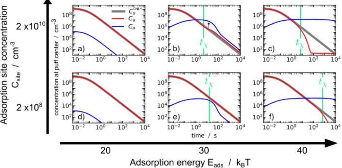
Figure 4.Concentration of pheromones at the center of the puff over time. These graphs illustrate that, after 102_{s, in most realistic cases, the}

majority of the tiny amount of emitted pheromones are adsorbed and transported asfinite ensembles by individual aerosols. Cgand Caare,

respectively, the concentration of gas and adsorbed pheromones. CgONLYis pheromone concentration when no aerosols are present, pheromones

remaining in the gas phase. tχis the time of the adsorption/desorption reaction (eq 10). When adsorption is favorable (high Eads and Csite),

adsorbed pheromones become predominant after some time. This slows down the decrease of concentrations due to diffusion. When adsorption is not favorable, only a small proportion of pheromones become adsorbed, and it does not modify the decrease of the concentration. Log scaled axis.

several hours, whereas gas diffusion would have widespread the molecules in a 1 m large domain. Aerosols keep the number of pheromones per volume of air at a high level over a long time and long distance of transport.

Figure 4 presents concentrations of adsorbed and gas pheromones at the center of the puff as functions of time. The relative importance of adsorption over the desorption process explains the various observed behaviors. For an adsorption energy (Eads) of 40 kBT (Figure 4c,f), the desorption is

quasinegligible, and Caincreases due to the adsorption process

at the same time as Cg decreases due to diffusion. The

concentration of absorbed pheromone (C_a) becomes higher than the concentration of gas pheromone (C_g) after some time. Then, pheromone concentration stops decreasing because they are mainly adsorbed on aerosols, which exhibit a slow diffusion. For Eads= 30 kBT and Csite= 2× 1010cm−3(Figure 4b), the

decreasing of pheromone concentrations is only delayed compared to a case where no aerosols would be present. This is due to two effects. First, the effective diffusivity (eq 23) is smaller than gas diffusion and takes place when the chemical equilibrium is reached. Second (see black arrow in the graph), as the center of the puff becomes depleted of gaseous pheromones, absorbed pheromones need to be desorbed for diffusion to continue. In other words, at a certain time (∼3 s), aerosols become excessively loaded in pheromones compared to the amount of gaseous pheromones around them so that desorption is limiting the dilution of pheromones. This effect leads here to a 10-fold increase in pheromone concentration at the center of the puff after few t_χ.

For Eads= 20 kBT (Figure 4a,d) and for Eads= 30 kBT and

Csite = 2 × 108 cm−3 (Figure 4e), desorption is mostly

dominant over adsorption, and no delay of the diffusion is observed as pheromones are mostly in the gas phase. For Eads=

30 k_BT and C_site= 2× 108_cm−3_{, a switch from the adsorbing to}

desorbing regime is also observable. For E_ads = 20 k_BT, chemical processes occur before gas diffusion takes place with very few molecules adsorbed, and equilibrium is instanta-neously adapted as diffusion occurs.

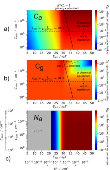
To finely describe the transition in parameter values for which pheromone adsorption on aerosols becomes significant, we plotted in Figure 5a,b the concentrations of gas and adsorbed pheromones at the center of a puff 100 s after its emission, as functions of Eads and Csite. Drastically different

behaviors can be observed whether adsorption energy is above or below 30 kBT. Above this threshold, a significant amount of

pheromones are adsorbed on aerosols, and C_aonly varies with adsorption site concentration (because it governs the adsorption process). The number of pheromones per aerosol

N C

C

a

a aero

= is also plotted inFigure 5c. It only slightly depends on the aerosol concentration (Caero). Indeed, physically, this

quantity does not directly depend on the aerosol concen-tration. This is due to the fact that a single aerosol equilibrates its number of adsorbed pheromones with the gas ones independently of how many aerosol neighbors it has. The only indirect dependence comes from the dynamics of the gas pheromone concentration (C_g) as can be shown by rewriting

eqs 15 and 16 in terms of the number of pheromones per aerosols (Na). At short times (t < tχ), Cg mainly exhibits a

diffusion process which does not depend on Caero(Figure 4).

Thus, Nadoes not depend on this quantity. At long times (t >

tχ) once the adsorption is made, the adsorptionflux becomes

very small (because of the low gas pheromone concentration), and Nadoes not depend on Caeroeither.

Aerosols are found to have as many as several thousands of pheromones on them for Eads > 30 kBT in the situation

described in Figure 5. Nevertheless, the maximal aerosol coverage that can be obtained is Ca/Csite = 0.09 ≪ 1,

confirming that saturation effects could be neglected. Finally, we demonstrated that, above a threshold for the adsorption energy, numerous pheromones are adsorbed on aerosols and maintain the pheromone concentrated for a long time; the threshold is typically for t = 100 s, E_ads = 30 k_BT, i.e., K0₌

10−10cm3.

Figure 5.Adsorbed pheromone concentration (Ca), gas pheromone

concentration (Cg), and number of adsorbed pheromones per aerosol

(Na) at the center of the puff 100 s after its emission. Eads and

Csite _SR C

4 aero

aero2 site

= π are, respectively, the adsorption energy and the concentration of adsorbing sites in the air. Caeroand K0= VseEadsare,

respectively, the aerosol concentration in the air and the Langmuir chemical constant. In Caand Cg graphs, two regions are observed,

roughly separated by the K0_C

site= 1 oblique axis. On the left side of

this axis, chemical equilibrium is reached; pheromones are mainly in the gas phase, and they diffuse through gas diffusion. On the right side of the K0_C

site= 1 axis, adsorbed pheromones dominate over gas ones.

In this region, below the tads _{k C} 100

1

ads site

= = s horizontal axis, chemical equilibrium is not reached. The Na _CCa

aero

= graph, was computed supposing that aerosols had a radius of 0.3μm. The initial puff concentration is CTi = 5× 109cm−3, and the initial puff radius is

■

A description of the aggregation dynamics of pheromones on the aerosol surface, unable to penetrate in the aerosol bulk, was achieved using the general framework introduced by Gibbs and refined by Tanford for the two-dimensional pseudophases created by amphiphilic molecules.4,19,26,43,44Occupancy of the surface by aerosols can be estimated with high precision as long as the gain of energy of moving the pheromone from the gas phase to the interface can be determined. Appropriated experimental and theoretical methods can lead to such results.27,45−48 We developed here the generic theory in the case of independent pheromone molecules adsorbed on the surface of aerosols composed of pure water.

We showed that the energy of adsorption strongly influence (threshold effect) the proportion of pheromones adsorbed at long time. We furthermore showed that aerosol concentration modifies the adsorption kinetics of the pheromones and thus the amount of pheromones that can diffuse through gas diffusion before becoming adsorbed. Aerosol concentration determines the time, or equivalently the distance from the source, at which the adsorbed pheromones overwhelm the gas ones and at which the diffusion of the pheromone puff switches from gas to effective diffusion. However, aerosol concentration does not significantly modify the number of pheromone molecules per aerosol.

As a consequence, as long as we have some adsorbing aerosols (with Eads> 30 kBT), many pheromones can be found

on each one of them. The aerosols become coated with pheromones quickly (less than 100 s) and can stay so for quite a long time in the air (>103_{s), while pheromones staying in}

the gas phase become dispersed to undetectable concen-trations rapidly due to gas diffusion. This distinction between molecular and aerosol transport mechanisms has great consequences in the way we picture the transport of pheromones. The spatial distribution of pheromones following molecular transport would be widespread, as a puff becomes larger and larger and less and less dense. By contrast, pheromones following aerosol transport would be distributed as dense spots, and hence strong olfactory clues, that last for a long time. As a consequence, many molecules, on a single aerosol, arriving on an insect at the same time might trigger an olfactory detection (Figure 6).

The number of molecules that can accumulate on the surface of one aerosol depends on relative humidity as it increases aerosol water content and size.15 More generally, humidity has been observed to influence moth pheromonal communication.49 Our general theory might offer the first clues to understand the mechanisms underlying these observations. Progress in this direction depends on exper-imental advances in order to characterize the molecules transported in one aerosol of control type and history.17,47 Proper characterization of aerosol surface composition and properties is still a challenging task and is limited to rare studies.17,18 Further investigation would need to discriminate which values of parameters are mostly fitting a specific chemical communication context.

More complex effects, beyond the description of adsorption of individual molecules at the pure water surface, might come into play in the aerosol transport of pheromones. Interactions with all surface-active species (i.e., organic and hydrophobic molecules, surfactants, hydrotropes, salts19,50−53) and espe-cially nanoparticles54 affect the content of the surface. Adsorbed species can either favor the adsorption of pheromones via a cosurfactant effect or hinder it due to crowding. Thus, strong antagonistic as well as synergistic effects are expected.19,51,53Other biogenic surfactants in the air can compete with pheromones for adsorption on aerosols and saturate the surface. Saturation of aerosols includes nonlinear effects in pheromone transport and hampers aerosol transport (seeAppendix B). Inhibition of the pheromonal response in given insects in the presence of specific plant volatiles has been reported.55 Saturation of aerosols by the plant volatiles47 or other physicochemical effects might reduce pheromone detection by the insects. Saturation of aerosols can also occur by smaller poorly labile aerosols, such as airborne solid carbon residues of combustion that are one major issue in large cities.14The number of small aerosols needed to saturate the surface of a bigger one is 4f2where f is the ratio between the radius of the bigger and small aerosols. For f = 10, it gives 400 small aerosols for every bigger one, a ratio which holds within polluted air records.14,15Moreover, adsorption on aerosol can increase pheromone degradation speed by collecting pher-omones and reactive species together at the surface.17,46,56,57 On the other hand, mixtures of surface-active molecules can be chosen with a specific blend so that their adsorption properties are enhanced.19,53Pheromones are known to often be released with accurate blend ratios,3,12 but there is no current

Figure 6.Illustration of antenna-pheromones encountering events for molecular and aerosol transport of pheromones (values given are only illustrative). (a) Encountering events of individual pheromones (red) and aggregated pheromones on aerosols (blue) with insect antenna. Encountering events are less frequent for aerosol transport, but many molecules arrive at the same time. (b) As the insect moves toward the source, the frequency of encountering events and number of pheromones associated evolve according to two scenarios. The red dashed curve is the scenario for pheromones following molecular transport only. The blue curve is for aerosol transport. In the shaded area, pheromones are not detected by the receptor insect because the number of molecules and the frequency of encounters are too low. In the case of aerosol transport, an insect starting far from the source (in the vertical part of the blue curve) only meets pheromones on aerosols. The number of pheromones per aerosol increases as the insect goes toward the source. In the oblique part of the blue curve, gas and adsorbed pheromones coexist as the insect is close enough to the source so that pheromones are not yet adsorbed by aerosols. Aerosol transport helps to maintain the pheromones at detectable levels.

explanation on how these blends could remain stable from emitter gland to receptor insect. Aggregation and synergistic effects might occur between the molecules of the blend and help to maintain a stable ratio between the molecules. Synergies can also occurs with other molecules released by plants in the insect habitat.47,55,56 Some effects favoring or hampering aerosol transport might be applied for the design of sustainable methods in pest control using volatile dispensers or multicropping systems.56,58 In the model we developed, the concentration of adsorption sites is the same everywhere in the air, and the adsorption energy does not vary from one site to another. In practice, these quantities inherentlyfluctuate. See theSupporting Information, section D, for further discussion on how our model relates to such a context.

Finally, we propose that certain molecules synthesized by insects for communicating evolved into molecules adapted to adsorb on the aerosols naturally present in the air. The concerned molecules use a communication path different from molecules staying in the gas phase and increase persistence of the signal in the air. Moreover, capture of aerosols by insect antennae differ from capture of individual molecules. Interaction between insect olfactory organs (sensilla) and aerosols might be governed by wetting and coalescing dynamics as well as colloidal and electrostatic interactions,26,59 enhancing the capture by increasing the cross-section area of the sensor.60,61 Accurate modeling of the pheromone path from release to reception in a way that explains observed performances of insect mate finding62 has not been reached yet. Pheromone uptake by aerosol has not been considered so far. We showed here that aerosol transport maintains olfactory clues over long distances (seeFigure 6) and is a new efficient channel for communication. The approach used here, inherited from the field of physicochemistry, was a key element to formulate this problem. A further understanding of interactions between olfactory molecules in the atmosphere in the frame of physicochemistry can have direct applications, in particular in the improvement of insect pest control, as well as fundamental consequences in the understanding of ecological interac-tions.3,63−66

■

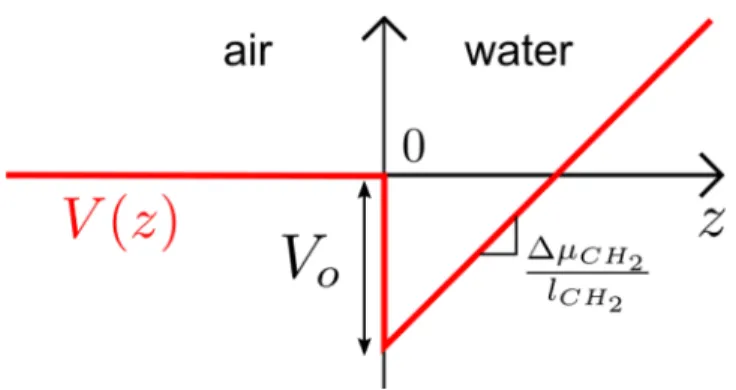
We consider surfactant molecules moving between the air and water interface. We aim to compute V(z), the free energy of a molecule at position z from the interface, averaged over on all the solvent configurations and molecule orientations (which corresponds to the McMillan−Mayer potential67). Following Ivanov and collaborators’ works,24,25we suppose that V(z) = 0 in the air for z < 0 and in the water for z > 0:

V z V l z ( ) 0 CH CH 2 2 μ = − + Δ (A1)

V0is the free energy gain when moving the molecule from gas

to the interface. l CH2 CH2 μ Δ

is the energy cost per unit of length when the molecule penetrates in the water phase as the carbon chain becomes hydrated. An illustration of this formula is given inFigure A1. V₀has several contributions:

V₀=E_head+ γS_site−F_rot=E_ads−F_rot (A2)

F_rot= k_BT ln 2 is the free energy (entropic) cost due to the fact that the molecule at the interface is constrained to rotate only

in a half space. Ehead and γSsite contributions were already

specified in the main text. Distribution of surfactant molecules is then given by C z( ) C exp

(

)

k T

g

( )

B

= − , and the surface

density of surfactants reads _a C z( ) dz

0

∫

The Langmuir equilibrium for low molecule density reads

K C

C C

0 a site g

= . The concentration of adsorbed pheromones and adsorption sites further reads C_a C_aero4 R

3 aero 2 a π = Γ and C C R S site aero 4 3 aero 2 site

= π so that their ratio is C S

C a site

a

site = Γ . Finally,

wefindK0=SsiteδeEads/k TB as given ineq 3.

■

TRANSPORT WHEN AEROSOLS CAN SATURATE Dynamics of pheromone transport in the case of saturating aerosols can be described within the frame of fast variable elimination.68The reaction-diffusioneqs 13and14are solved within the limit of fast chemistry: kabs→ +∞. Caand Cgare fast

variables because C t a ∂ ∂ and C t g → +∞ ∂

∂ within this limit. On the

other hand the total pheromone concentration C_T = C_a+ C_g follows C t (D C D C) T g g a a ∇ ∇ ∇ ∂ ∂ = · + (A4) and C t T ∂

∂ does not diverge when kabs → +∞. CT can be

considered as a slow variable for which the evolution is much slower than the one of C_a and C_g. Instantaneously, the fast variables Caand Cg react, and they follow the variation of the

slow variable C_T. This slavery of C_a and C_g is valid if one considers time scales longer than the chemical scale t≫ tχ. In

that case, the distribution ratio of gas and adsorbed pheromones adapt locally to equilibrium value on a time scale way shorter than the one with which C_Tevolves. It is thus fixed byeq 1and the local value of CT. We replace Cgand Ca

by C_g(C_T) and C_a(C_T) in eq A4tofind C t (D (C ) C ) T eff T T ∇ ∇ ∂ ∂ = · (A5) with

Figure A1.Free energy profile of the nonsoluble surfactant at the waterair interface, following Ivanov and collaborators.24,25

D C D C C D C C ( ) d d d d eff T g g T a a T = + (A6)

These general formulas mean that the pheromone transport follows a space-dependent Fick’s law for which the local diffusion coefficient is Deff. For nonsaturating aerosols,

equilibrium reduces to C K C C 0 s g a

= , and we recover the result given in eq 23. The effective diffusion coefficient of the pheromone is an average of the one of the gas and the aerosol. On the other hand, for saturated aerosols, C_a= C_sand C_g= C_T − Csso that Deff= Dg. The saturation of the aerosols prevents

them from retaining the pheromones. At any time, as soon as the aerosols are saturated, they can no longer store the molecules which then diffuse with the gas diffusion coefficient. The containment of pheromones during transport by means of aerosols can therefore only take place as long as the aerosols are not saturated.

■

*

The Supporting Information is available free of charge at

https://pubs.acs.org/doi/10.1021/acscentsci.0c00892. Results when adsorption kinetics is limited, further justifications of the applicability of a linear model, data showing the negligible influence of the varying aerosol diffusion coefficient, and a discussion on how our model relates to a realisticfluctuating environment (PDF)

■

Corresponding Author

Jean-François Dufrêche − ICSM, CEA, CNRS, ENSCM, Univ Montpellier, 30207 Bagnols-sur-Cèze, France; orcid.org/ 0000-0001-8422-3639; Email:jean-francois.dufreche@ umontpellier.fr

Authors

Ludovic Jami − ICSM, CEA, CNRS, ENSCM, Univ Montpellier, 30207 Bagnols-sur-Cèze, France; orcid.org/ 0000-0002-8822-7669

Thomas Zemb − ICSM, CEA, CNRS, ENSCM, Univ Montpellier, 30207 Bagnols-sur-Cèze, France; orcid.org/ 0000-0001-8410-6969

Jérôme Casas − Institut de Recherche sur la Biologie de l’Insecte, UMR 7261, CNRSUniversité de Tours, 37200 Tours, France; orcid.org/0000-0003-1666-295X

Complete contact information is available at:

https://pubs.acs.org/10.1021/acscentsci.0c00892

Author Contributions

All the authors planned together this research work. L.J. and J.-F.D. conducted the modeling. J.C. and T.Z. provided data and analysis from, respectively, insect ecology and microphases’ physicochemistry. L.J. wrote the manuscript, and all authors contributed to its editing.

Notes

The authors declare no competingfinancial interest.

■

We thank Claudio Lazzari, Christophe Bressac, Lolita Hilaire, and Bertrand Siboulet for fruitful discussions. The work was supported by the Project PHEROAERO from the Region

Centre and by a ENS Lyon Ph.D. fellowship to L.J. in Tours under the supervision of J.C. and J.-F.D.

■

(1) Bossert, W. H.; Wilson, E. O. The analysis of olfactory communication among animals. J. Theor. Biol. 1963, 5, 443−469.

(2) Murlis, J.; Elkinton, J. S.; Carde, R. T. Odor plumes and how insects use them. Annu. Rev. Entomol. 1992, 37, 505−532.

(3) Pannunzi, M.; Nowotny, T. Odor stimuli: Not just chemical identity. Front. Physiol. 2019, 10, 1428.

(4) Kronberg, B.; Holmberg, K.; Lindman, B. Surface chemistry of surfactants and polymers; John Wiley & Sons, 2014.

(5) Kunz, W.; Holmberg, K.; Zemb, T. Hydrotropes. Curr. Opin. Colloid Interface Sci. 2016, 22, 99−107.

(6) Schöttl, S.; Horinek, D. Aggregation in detergent-free ternary mixtures with microemulsion-like properties. Curr. Opin. Colloid Interface Sci. 2016, 22, 8−13.

(7) Regnier, F. E.; Law, J. H. Insect pheromones. J. Lipid Res. 1968, 9, 541−551.

(8) chemspider.http://www.chemspider.com(accessed 2020-04-09). (9) Ando, T.; Inomata, S.-i.; Yamamoto, M. The chemistry of pheromones and other Semiochemicals I; Springer, 2004; pp 51−96.

(10) Krasnoff, S. B.; Roelofs, W. L. Sex pheromone released as an aerosol by the moth Pyrrharctia isabella. Nature 1988, 333, 263−265. (11) Kuba, H.; Sokei, Y. The production of pheromone clouds by spraying in the melon fly, Dacus cucurbitae Coquillett (Diptera: Tephritidae). Journal of Ethology 1988, 6, 105−110.

(12) Schal, C.; Charlton, R. E.; Cardé, R. T. Temporal patterns of sex pheromone titers and release rates in Holomelina lamae (Lepidoptera: Arctiidae). J. Chem. Ecol. 1987, 13, 1115−1129.

(13) Jaenicke, R. Natural aerosols. Ann. N. Y. Acad. Sci. 1980, 338, 317−329.

(14) Jaenicke, R. International Geophysics; Elsevier, 1993; Vol. 54, pp 1−31.

(15) Friedlander, S. K.; et al. Smoke, dust, and haze; Oxford University Press: New York, 2000; Vol. 198.

(16) Carslaw, K.; Boucher, O.; Spracklen, D.; Mann, G.; Rae, J.; Woodward, S.; Kulmala, M. A review of natural aerosol interactions and feedbacks within the Earth system. Atmos. Chem. Phys. 2010, 10, 1701.

(17) Donaldson, D.; Vaida, V. The influence of organic films at the air- aqueous boundary on atmospheric processes. Chem. Rev. 2006, 106, 1445−1461.

(18) Tervahattu, H.; Juhanoja, J.; Vaida, V.; Tuck, A.; Niemi, J. V.; Kupiainen, K.; Kulmala, M.; Vehkamäki, H. Fatty acids on continental sulfate aerosol particles. J. Geophys. Res. 2005, 110, D06207.

(19) Li, S.; Cheng, S.; Du, L.; Wang, W. Establishing a model organic film of low volatile compound mixture on aqueous aerosol surface. Atmos. Environ. 2019, 200, 15−23.

(20) Claeys, M.; Graham, B.; Vas, G.; Wang, W.; Vermeylen, R.; Pashynska, V.; Cafmeyer, J.; Guyon, P.; Andreae, M. O.; Artaxo, P.; et al. Formation of secondary organic aerosols through photo-oxidation of isoprene. Science 2004, 303, 1173−1176.

(21) Rizzo, L.; Artaxo, P.; Karl, T.; Guenther, A.; Greenberg, J. Aerosol properties, in-canopy gradients, turbulent fluxes and VOC concentrations at a pristine forest site in Amazonia. Atmos. Environ. 2010, 44, 503−511.

(22) Pöhlker, C.; Wiedemann, K. T.; Sinha, B.; Shiraiwa, M.; Gunthe, S. S.; Smith, M.; Su, H.; Artaxo, P.; Chen, Q.; Cheng, Y.; et al. Biogenic potassium salt particles as seeds for secondary organic aerosol in the Amazon. Science 2012, 337, 1075−1078.

(23) Zhu, C.; Kawamura, K.; Fukuda, Y.; Mochida, M.; Iwamoto, Y. Fungal spores overwhelm biogenic organic aerosols in a midlatitudinal forest. Atmos. Chem. Phys. 2016, 16, 7497−7506.

(24) Slavchov, R. I.; Ivanov, I. B. Effective osmotic cohesion due to the solvent molecules in a delocalized adsorbed monolayer. J. Colloid Interface Sci. 2018, 532, 746−757.

(25) Slavchov, R. I.; Ivanov, I. B. Adsorption parameters and phase behaviour of non-ionic surfactants at liquid interfaces. Soft Matter 2017, 13, 8829−8848.

(26) Israelachvili, J. N. Intermolecular and surface forces; Academic press, 2015.

(27) Liyana-Arachchi, T. P.; Zhang, Z.; Vempati, H.; Hansel, A. K.; Stevens, C.; Pham, A. T.; Ehrenhauser, F. S.; Valsaraj, K. T.; Hung, F. R. Green leaf volatiles on atmospheric air/water interfaces: A combined experimental and molecular simulation study. J. Chem. Eng. Data 2014, 59, 3025−3035.

(28) Marek, R.; Straub, J. Analysis of the evaporation coefficient and the condensation coefficient of water. Int. J. Heat Mass Transfer 2001, 44, 39−53.

(29) Tsuruta, T.; Nagayama, G. A microscopic formulation of condensation coefficient and interface transport phenomena. Energy 2005, 30, 795−805.

(30) Nagayama, G.; Takematsu, M.; Mizuguchi, H.; Tsuruta, T. Molecular dynamics study on condensation/evaporation coefficients of chain molecules at liquid−vapor interface. J. Chem. Phys. 2015, 143, No. 014706.

(31) Persad, A. H.; Ward, C. A. Expressions for the evaporation and condensation coefficients in the Hertz-Knudsen relation. Chem. Rev. 2016, 116, 7727−7767.

(32) Varilly, P.; Chandler, D. Water evaporation: A transition path sampling study. J. Phys. Chem. B 2013, 117, 1419−1428.

(33) Julin, J.; Shiraiwa, M.; Miles, R. E.; Reid, J. P.; Pöschl, U.; Riipinen, I. Mass accommodation of water: Bridging the gap between molecular dynamics simulations and kinetic condensation models. J. Phys. Chem. A 2013, 117, 410−420.

(34) Julin, J.; Winkler, P. M.; Donahue, N. M.; Wagner, P. E.; Riipinen, I. Near-unity mass accommodation coefficient of organic molecules of varying structure. Environ. Sci. Technol. 2014, 48, 12083−12089.

(35) Bley, M.; Duvail, M.; Guilbaud, P.; Dufrêche, J.-F. Simulating Osmotic Equilibria: A New Tool for Calculating Activity Coefficients in Concentrated Aqueous Salt Solutions. J. Phys. Chem. B 2017, 121, 9647−9658.

(36) Zwanzig, R. Nonequilibrium Statistical Mechanics; Oxford University Press, 2001.

(37) Pöschl, U.; Rudich, Y.; Ammann, M. Kinetic model framework for aerosol and cloud surface chemistry and gas-particle interactions ? Part 1: General equations, parameters, and terminology. Atmos. Chem. Phys. 2007, 7, 5989−6023.

(38) Umbers, K. D. L.; Symonds, M. R. E.; Kokko, H. The Mothematics of Female Pheromone Signaling: Strategies for Aging Virgins. Am. Nat. 2015, 185, 417−432.

(39) Foster, S. P.; Anderson, K. G.; Casas, J. The dynamics of pheromone gland synthesis and release: a paradigm shift for understanding sex pheromone quantity in female moths. J. Chem. Ecol. 2018, 44, 525−533.

(40) Bird, R. B.; Stewart, W. E. Transport phenomena, 2nd ed.; John Wiley & Sons, 2007; Chapter 19, pp 582−606.

(41) Turq, P.; Barthel, J.; Chemla, M. Transport, Relaxation and Kinetic Processes in Electrolyte Solutions; Springer-Verlag, 1992.

(42) Berne, B. J.; Pecora, R. Dynamic Light Scattering; Dover, 2000. (43) Tanford, C. Hydrophobic free energy, micelle formation and the association of proteins with amphiphiles. J. Mol. Biol. 1972, 67, 59−74.

(44) Tanford, C. The hydrophobic effect: formation of micelles and biological membranes, 2nd ed; J. Wiley, 1980.

(45) Massoudi, R.; King, A., Jr Effect of pressure on the surface tension of water. Adsorption of low molecular weight gases on water at 25. deg. J. Phys. Chem. 1974, 78, 2262−2266.

(46) Valsaraj, K. T. A review of the aqueous aerosol surface chemistry in the atmospheric context. Open J. Phys. Chem. 2012, 2 (1), 58.

(47) Ren, Y.; McGillen, M.; Daële, V.; Casas, J.; Mellouki, W. The fate of methyl salicylate in the environment and its role as signal in multitrophic interactions. Sci. Total Environ. 2020, 141406.

(48) De Angelis, P.; Cardellini, A.; Asinari, P. Exploring the Free Energy Landscape To Predict the Surfactant Adsorption Isotherm at the Nanoparticle−Water Interface. ACS Cent. Sci. 2019, 5, 1804− 1812.

(49) McNeil, J. N. Behavioral ecology of pheromone-mediated communication in moths and its importance in the use of pheromone traps. Annu. Rev. Entomol. 1991, 36, 407−430.

(50) Kunz, W. Specific ion effects; World Scientific, 2010.

(51) Demou, E.; Donaldson, D. Adsorption of atmospheric gases at the air- water interface. 4: The influence of salts. J. Phys. Chem. A 2002, 106, 982−987.

(52) Brzozowska, A.; Duits, M. H.; Mugele, F. Stability of stearic acid monolayers on Artificial Sea Water. Colloids Surf., A 2012, 407, 38−48.

(53) Špadina, M.; Bohinc, K.; Zemb, T.; Dufrêche, J.-F. Synergistic Solvent Extraction Is Driven by Entropy. ACS Nano 2019, 13, 13745−13758.

(54) Binks, B. P.; Yin, D. Pickering emulsions stabilized by hydrophilic nanoparticles: in situ surface modification by oil. Soft Matter 2016, 12, 6858−6867.

(55) Reddy, G. V.; Guerrero, A. Interactions of insect pheromones and plant semiochemicals. Trends Plant Sci. 2004, 9, 253−261.

(56) Conchou, L.; Lucas, P.; Meslin, C.; Proffit, M.; Staudt, M.; Renou, M. Insect odorscapes: from plant volatiles to natural olfactory scenes. Front. Physiol. 2019, 10, 972.

(57) Donaldson, D.; Valsaraj, K. T. Adsorption and reaction of trace gas-phase organic compounds on atmospheric water film surfaces: A critical review. Environ. Sci. Technol. 2010, 44, 865−873.

(58) Mofikoya, A. O.; Bui, T. N. T.; Kivimäenpää, M.; Holopainen, J. K.; Himanen, S. J.; Blande, J. D. Foliar behaviour of biogenic semi-volatiles: potential applications in sustainable pest management. Arthropod-Plant Interactions 2019, 13, 193−212.

(59) Carroll, B. The accurate measurement of contact angle, phase contact areas, drop volume, and Laplace excess pressure in drop-on-fiber systems. J. Colloid Interface Sci. 1976, 57, 488−495.

(60) Jaffar-Bandjee, M.; Steinmann, T.; Krijnen, K.; Casas, J. Leakiness and flow capture rate ratio of insect pectinate antenna. J. R. Soc., Interface 2020, 17, 20190779.

(61) Spencer, T. L.; Mohebbi, N.; Jin, G.; Forister, M. L.; Alexeev, A.; Hu, D. L. Moth-inspired methods for particle capture on a cylinder. J. Fluid Mech. 2020, 884, 927.

(62) Wall, C.; Perry, J. Range of action of moth sex-attractant sources. Entomol. Exp. Appl. 1987, 44, 5−14.

(63) Koehl, M. Physical modelling in biomechanics. Philos. Trans. R. Soc., B 2003, 358, 1589−1596.

(64) Denny, M. Ecological mechanics: Principles of life’s physical interactions; Princeton University Press, 2015.

(65) Yohe, L. R.; Brand, P. Evolutionary ecology of chemosensation and its role in sensory drive. Curr. Zool. 2018, 64, 525−533.

(66) Katsnelson, A. Decoding an Insects Sensory World. ACS Cent. Sci. 2018, 4, 785.

(67) McMillan, W. G., Jr; Mayer, J. E. The statistical thermody-namics of multicomponent systems. J. Chem. Phys. 1945, 13, 276− 305.

(68) Van Kampen, N. G. Elimination of fast variables. Phys. Rep. 1985, 124, 69−160.