A Semi-automatic Proof of Strong connectivity

HAL Id: hal-01632947

https://hal.inria.fr/hal-01632947

Submitted on 10 Nov 2017

HAL is a multi-disciplinary open access

archive for the deposit and dissemination of

sci-entific research documents, whether they are

pub-lished or not. The documents may come from

teaching and research institutions in France or

L’archive ouverte pluridisciplinaire HAL, est

destinée au dépôt et à la diffusion de documents

scientifiques de niveau recherche, publiés ou non,

émanant des établissements d’enseignement et de

recherche français ou étrangers, des laboratoires

A Semi-automatic Proof of Strong connectivity

Ran Chen, Jean-Jacques Lévy

To cite this version:

Ran Chen, Jean-Jacques Lévy. A Semi-automatic Proof of Strong connectivity. 9th Working

Confer-ence on Verified Software: Theories, Tools and Experiments (VSTTE), Jul 2017, Heidelberg, Germany.

�hal-01632947�

A Semi-automatic Proof of Strong connectivity

1

Inria Saclay & Iscas Beijing chenr@ios.ac.cn 2

Inria Paris jean-jacques.levy@inria.fr

Abstract. We present a formal proof of the classical Tarjan-1972 algo-rithm for finding strongly connected components in directed graphs. We use the Why3 system to express these proofs and fully check them by computer. The Why3-logic is a simple multi-sorted first-order logic aug-mented by inductive predicates. Furthermore it provides useful libraries for lists and sets. The Why3 system allows the description of programs in a Why3-ML programming language (a first-order programming language with ML syntax) and provides interfaces to various state-of-the-art au-tomatic provers and to manual interactive proof-checkers (we use mainly Coq). We do not claim that this proof is new, although we could not find a formal proof of that algorithm in the literature. But one important point of our article is that our proof is here completely presented and human readable.

1

Introduction

Formal proofs about programs are often very long and have to face a huge amount of cases due to the multiplicity of variables, the details of programs, and the description of their meta-theories. This is very frustrating since we would like to explain these formal proofs and publish them in scientific articles. However if one considers simple algorithms, we would expect to explain their proofs of correctness in the same way as we explain a mathematical proof for a not too complex theorem. This surely can be done on algorithms dealing with simple recursive structures [5, 29, 19]. But we take here the example of an algorithm on graphs where sharing and combinatorial properties holds.

Tarjan-1972’s algorithm for finding strongly connected components in di-rected graphs is very magic [26, 1, 24]. It consists in an efficient depth-first search in graphs which traces the bases of the strongly connected components. It com-putes in linear time the strongly connected components. In textbooks, the pre-sentation uses an imperative programming style that we will refresh in section 2, but for the sake of the simplicity of the proof, we will describe this algorithm in a functional programming style with abstract values for vertices in graphs, with functions between vertices and their successors, and with data types such that lists (representing immutable stacks) and sets. This programming style will much ease the readability of our formal proof.

?

Partly supported by ANR-13-LAB3-0007, http://www.spark-2014.org/proofinuse and National Natural Science Foundation of China (Grant No. 61672504)

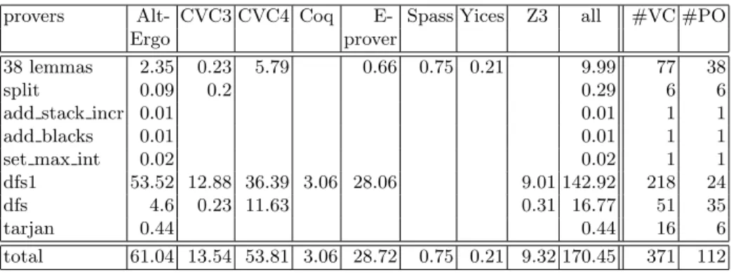
We use the Why3 system [14, 3] and the Why3-logic to express these proofs. Our proof is rather short, namely 235 lines (38 lemmas) including the pro-gram texts. Most of the lemmas and the 74 proof obligations generated by the Why3 system for our program are proved automatically using Alt-Ergo (1.30), CVC3 (2.4.1), CVC4 (1.5-prerelease), Eprover (1.9), Spass (3.5), Yices (1.0.4), Z3 (4.4.0) except 2 of them which are manually checked by Coq (8.6) with a few ssreflect features [13, 15]. Coq proofs are 233-line long (65 + 168).

Our claim is that the details of our proof are human readable and intuitive. The proof will be fully described in our paper. Therefore it could be an example of teaching algorithms with their formal proofs. Finally our article can present a useful step to compare with other formal methods, for instance within Isabelle or Coq [22, 18, 28, 27, 16, 6, 8, 7, 2, 21, 20].

The next section will present the algorithm; section 3 and 4 present the invariants and pre-/post-conditions, section 5 describes the formal proof. We conclude in section 6.

2

The algorithm

A strongly connected component in a directed graph is a nonempty maximal set of vertices in which any pair of vertices can be joined by a path. Therefore when two vertices x and y are in such a component, there exist paths from x to y and from y to x. In the rest of the paper we shall just say connected components for strongly connected components.

Tarjan-1972 algorithm [26, 1, 24] for finding (strongly) connected components in a directed graph performs a single depth-first search traversal. It maintains a stack of visited vertices and a numbering of vertices. Initially the stack is empty and the serial number of all vertices is −1. Then vertices get increasing serial numbers in the order of their visit. Each vertex is visited once. The search is realized by a recursive function which starts from any unvisited vertex x, pushes it on the stack, visits the directly reachable vertices from x, and returns the minimum value of the numbers of all vertices accessible from x by at most one cross-edge. A cross-edge is an edge between an unvisited vertex and an already visited vertex. If there is no such edge, the returned value is +∞. When the returned value is equal to the number of x, a new component cc containing x is found and all vertices of cc are then at top of the stack, x being the low-est. Therefore the stack is popped until x and the numbers of the component members are set to +∞, which withdraws them from further calculations in the following visits of vertices.

To make this algorithm more explicit, we consider the below recursive func-tion printSCC which prints the connected components reachable from any given vertex x and returns an integer. It works with a given stack s, an array num of numbers, and a current serial number sn. The program written in two columns adopts a syntax close to the one of (Why3-)ML. The set of vertices directly reachable from vertex x by a single edge is represented by the set (successors x). This set can be implemented by a list of integers. We suppose that initially

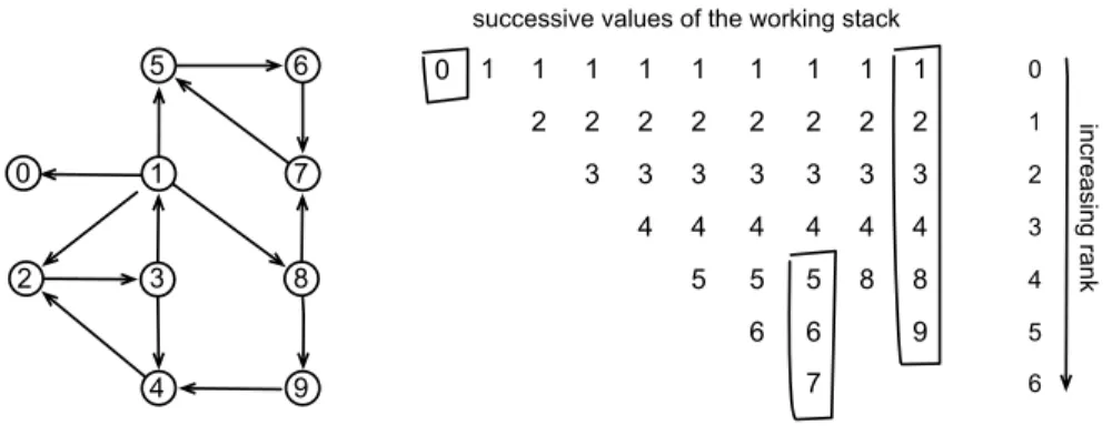
1 1 1 1 1 2 2 2 2 3 3 3 4 4 5 1 2 3 4 5 6 1 1 2 2 3 3 4 4 8 8 1 2 3 4 5 6 9 7 successive values of the working stack

0 1 2 3 4 5 6 in cre asi ng ra nk 2 3 8 4 9 1 7 5 6 0 0

Fig. 1. An example: in the graph on left, vertices are numbered and pushed onto the stack in the order of their visit by the recursive function printSCC. When the first component {0} is discovered, vertex 0 is popped; similarly when the second component {5, 6, 7} is found, its vertices are popped; finally all vertices are popped when the third component {1, 2, 3, 4, 8, 9} is found. Notice that there is no cross edge to a vertex with a number less than 5 when the second component is discovered. Similarly in the first component, there is no edge to a vertex with a number less than 0. In the third component, there is no edge to a vertex less than 1 since we then set the number of vertex 0 to +∞.

sn is set to 0 and that all entries in num are equal to −1. The constant max int represents +∞. Figure 1 provides an example of execution of that function.

let rec printSCC (x: int) (s: stack int) (num: array int) (sn: ref int) = Stack.push x s;

num[x] ← !sn; sn := !sn + 1;

let min = ref num[x] in foreach y in (successors x) do

let m = if num[y] = -1

then printSCC y s num sn

else num[y] in

min := Math.min m !min

done;

if !min = num[x] then begin repeat let y = Stack.pop s in Printf.printf "%d " y; num[y] ← max_int; if y = x then break; done; Printf.printf "\n"; min := max_int; end; return !min;

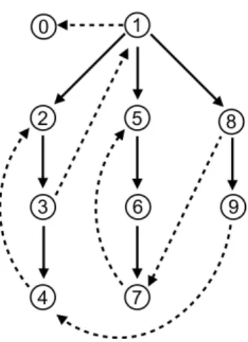
The proof of correctness of this algorithm in original Tarjan’s article relies on the structure of the connected components with respect to the spanning tree (forest) corresponding to the recursive calls of printSCC. A first lemma (Lemma 10 in the paper) states that if x and y are in a same component, their smallest common ancestor (i.e. the one with highest number) in the spanning tree is also in the same component. Therefore a connected component is always contained in one subtree of the spanning forest. The root of that minimum subtree is called the base of the component (Tarjan named it the root). Therefore the algorithm is designed to discover the bases of connected components. Lemma 12 proves that a vertex x is a base of a connected component if and only if the number

Fig. 2. Spanning forest: LOWLINK(x) is 0, 1, 1, 1, 2, 5, 5, 5, 4, 4 for 0 ≤ x ≤ 9

of x is equal to the value of so-called LOWLINK(x), which corresponds to the value computed by printSCC with x as input.

LOWLINK(x) = min ( {num[x]} ∪ {num[y] | x=⇒ z ,→ y∗

∧ x and y are in the same connected component} ) where x =⇒ z means that z is a descendant of x in the spanning forest and∗ z ,→ y means that there is a cross-edge from z to y (that is either an edge to an ancestor y of x, or to a cousin y of x, or to a descendant y of a child of x). Notice that in the second case, cousin y could only be at left of x in the spanning tree. The trick of the algorithm is that the LOWLINK function can be simply calculated through a single depth-first-search.

The proof of that Lemma 12 is about spanning trees and not about the recursive function which implements the depth-first-search. In order to make a formal proof of the algorithm, we may either formalize spanning trees and extract a program from these formal specifications, or directly manipulate the program and adapt the previous abstract proof to the various steps of this program. We prefer the latter alternative which is more speaking to a programmer and maybe easier to understand.

Our program will be expressed in a functional programming style. Thus we avoid side-effects and mutable variables. This Why3-ML program is based on two mutually recursive functions dfs1 and dfs which respectively take as arguments a vertex x and a set of vertices roots, and which return the number n of the oldest vertex accessible by at most one cross-edge. Both functions work with an environment represented by a record with four fields: stack for the working stack, sccs for the set of already computed connected components, sn for the current available serial number and num for the numbering mapping. The environment at end of both functions is also returned in their results. Thus the result of dfs1 and dfs is a pair (n, e0) where n is the number of the oldest vertex accessible

by at most one cross-edge and e’ is the environment at end of these functions. The main program tarjan calls dfs with all vertices as roots and an empty environment, i.e. an empty stack, an empty set of connected components, a null serial number and a constant mapping of vertices to −1.

let rec dfs1 x e =

let n = e.sn in

let (n1, e1) = dfs (successors x) (add_stack_incr x e) in let (s2, s3) = split x e1.stack in

if n1 < n then (n1, e1) else

(max_int(), {stack = s3; sccs = add (elements s2) e1.sccs; sn = e1.sn; num = set_max_int s2 e1.num})

with dfs roots e = if is_empty roots then (max_int(), e) else let x = choose roots in

let roots’ = remove x roots in

let (n1, e1) = if e.num[x] 6= -1 then (e.num[x], e) else dfs1 x e in let (n2, e2) = dfs roots’ e1 in (min n1 n2, e2)

let tarjan () =

let e0 = {stack = Nil; sccs = empty; sn = 0; num = const (-1)} in let (_, e’) = dfs vertices e0 in e’.sccs

The data structures used by these functions are the ones of the Why3 stan-dard library. For lists we have the constructors Nil, Cons and the function el-ements which returns the set of elel-ements of a list. For finite sets, we have the empty set empty, and functions add to add an element to a set, remove to re-move an element from a set, choose to pick an element in a set, and cardinal, is empty with intuitive meanings. We also use maps (instead of mutable arrays) with functions const denoting the constant function, [] to get the value of an element and [←] to create a new map with an element set to a given value. Thus we can define an abstract type vertex for vertices and a constant vertices for the finite set of all vertices in the graph. The type env of environments is a record with the four fields stack, sccs, sn and num whose meanings were stated above.

type vertex

constant vertices: set vertex

function successors vertex : set vertex

function max_int (): int = cardinal vertices

type env = {stack: list vertex; sccs: set (set vertex); sn: int; num: map vertex int}

Finally the function dfs1 uses the following three functions. Two of them handle environments: add stack incr pushes a vertex on the stack and sets its number to the value of the current serial number which is then incremented, set max int sets all the elements of a stack to max int(). The polymorphic func-tion split returns the pair of sublists produced by decomposing a list with respect to the first occurrence of an element.

{stack = Cons x e.stack; sccs = e.sccs; sn = n+1; num = e.num[x ← n]}

let rec set_max_int (s : list vertex)(f : map vertex int) =

match s with

| Nil → f

| Cons x s’ → (set_max_int s’ f)[x ← max_int()]

end

let rec split (x : α) (s: list α) : (list α, list α) =

match s with

| Nil → (Nil, Nil)

| Cons y s’ → if x = y then (Cons x Nil, s’) else let (s1’, s2) = split x s’ in ((Cons y s1’), s2)

end

We will assume that the imperative program printSCC behaves as the func-tions dfs1 and dfs. Our formal proof will only work on these two funcfunc-tions. We experimented several formal proofs of imperative versions, but they always looked over-complex (that complexity is mainly notational, since one always has to refer to the value of a variable at a given point of the program). To be convinced that the functions dfs1 and dfs follow the algorithm in the original paper, we notice that instead of printing the connected components, we accu-mulate them in the sccs field of environments and produce them as the result of the main function tarjan. We also use dfs to recursively execute the iterative loop of printSCC. The heart of the algorithm is in the body of function dfs1 where we split the working stack with respect to the vertex x giving two lists s2 and s3 (the last element of s2 is x ). Then we test if the elements of s2 forms a new connected component. In fact this test could be done before splitting, but the formal proof looks clearer if we keep them in that order.

Notice a small modification between our presentation and the one of the original version. In dfs1, we test n1 < n instead of n1 6= n. In the imperative program, the minimum is initialized to the number of x. Thus this initial value is used for two distinct purposes: the case when x is the root of a new connected component and the case when x is the top of the working stack. In the latter case we prefer returning +∞ for dfs which corresponds to the simpler formula E .

LOWLINK(x) = min {num[y] | x=⇒ z ,→ y∗ (E )

∧ x and y are in the same connected component} A final remark is that we could have inlined dfs1 in dfs or transformed the call to dfs1 into a call to dfs with a singleton set of roots as argument. Both alternatives do not simplify the proof, nor the invariants. Altogether we feel our presentation easier to read.

3

Invariants

This algorithm collects connected components in the sccs field of environments and we have to maintain that property along the execution of the program.

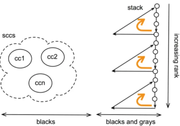
Fig. 3. Invariants on colors and stack

Partial connected components are contained in the working stack, and as soon as they are complete, they are moved from the stack to the sccs field. These partial connected components are connected components of the graph restricted to the elements of the stack and the sccs field, that is up to the already explored subgraph. These partial connected components are merged as soon as a back edge may access to an older ancestor in the spanning tree. This notion is not easy to manipulate since we would have also to mark the edges that we have visited. Therefore we break that property into several smaller pieces.

First we have to speak of the explored vertices. The num field marks visited vertices when their num value is not −1. There are two kinds of visited vertices as in any depth-first-search algorithm. The black vertices are fully explored by the algorithm, namely the call of dfs1 has been totally performed on them. The gray vertices are partially explored by that function, and the algorithm has still to visit several of its descendants in the spanning tree. The gray vertices represent the call stack of the recursive function dfs1. The non-visited vertices are said white, they correspond to a num field equals to −1 in the environment. The connected components are either fully black and are then members of the sccs field, or they contain a gray vertex, or are fully white. A gray vertex can access to any vertex pushed after it in the working stack (i.e. before in the list representing the stack). Conversely any vertex in the stack can access to a gray vertex pushed in the stack before it (i.e after in the list representing the stack). This invariant property of the stack and environment is illustrated in Figure 3 and can be checked on the example of Figures 1-2.

We now define formally the invariants. The graph is defined with an abstract type vertex for the type of vertices, a constant vertices for the set of all vertices in the graph, a function successors giving the set of vertices directly reachable by a single edge (see section 2). We also have the following axiom and definition:

axiom successors_vertices:

∀x. mem x vertices → subset (successors x) vertices

where mem and subset are the predicates denoting the membership in a set and the subset relation between two sets. Therefore edge is the binary relation defining the graph. The Why3 standard library defines paths in graphs as an inductive predicate and we also use a reachability predicate:

inductive path vertex (list vertex) vertex = | Path_empty: ∀x: vertex. path x Nil x | Path_cons: ∀x y z: vertex, l: list vertex.

edge x y → path y l z → path x (Cons x l) z

predicate reachable (x y: vertex) = ∃l. path x l y

Strongly connected components are naturally defined as non-empty maximal sets of vertices connected in both ways by paths.

predicate in_same_scc (x y: vertex) = reachable x y ∧ reachable y x

predicate is_subscc (s: set vertex) =

∀x y. mem x s → mem y s → in_same_scc x y

predicate is_scc (s: set vertex) = not is_empty s ∧

is_subscc s ∧ (∀s’. subset s s’ → is_subscc s’ → s == s’)

The colors of vertices are defined by membership to two sets: blacks and grays for the set of black and gray vertices. A white vertex is neither in blacks, nor in grays. (The grays set can also be implicit, since gray vertices are the non-black elements of the working stack, but we feel simpler to keep it explicit). These two sets blacks and grays are ghost variables for the Why3-ML program. They are used inside the logic of the proof, but they affect neither the control flow, nor the result of the program. We will treat them differently since blacks will be a new ghost field in environments and grays will be an extra ghost argument to the functions dfs1, dfs and tarjan. Adding the gray set as another new field of environments was intractable in the proof. We will discuss that point later. Thus the new type of environments is as follows:

type env = {ghost blacks: set vertex; stack: list vertex;

sccs: set (set vertex); sn: int; num: map vertex int}

and the main invariant (I) of our program will be: (I)

wf_env e grays ∧ ∀cc. mem cc e.sccs ↔ subset cc e.blacks ∧ is_scc cc

where wf env defines a well formed environment and the other conjunct specifies that the black connected components are exactly the elements of the sccs field. The definition of a well formed environment is done in three steps. First we define a well formed coloring: the grays and blacks sets are disjoint subsets of vertices in the graph; the elements of the stack is the union of grays and the difference of blacks and the union of elements of sccs; the elements of sccs are all black. The operations union, inter, diff on sets are defined in the Why3 standard library. But we had to define the big union set of axiomatically.

predicate wf_color (e: env) (grays: set vertex) =

let {stack = s; blacks = b; sccs = ccs} = e in

elements s == union grays (diff b (set_of ccs)) ∧ subset (set_of ccs) b

In the next two steps, we use two new predicates and a new definition. The no black to white predicate states that there is no edge from a black vertex to a white vertex. Any depth-first search respects that property since the black set is saturated by reachability. The simplelist predicate says that a list has no repetitions i.e. there is no more than one occurrence of any element. Our working stack satisfies that predicate since any vertex is visited no more than once. (The num occ function belongs to the Why3 standard library)

predicate no_black_to_white (blacks grays: set vertex) =

∀x x’. edge x x’ → mem x blacks → mem x’ (union blacks grays)

predicate simplelist (l: list α) = ∀x. num_occ x l ≤ 1

The rank function gives the position of an element in a list starting from the end of the list. In a working stack of length `, the ranks of the bottom and top of the stack are 0 and ` − 1 (see Figures 1 and 3). The rank function allows to order vertices in the stack with respect to their positions. It could be done just with numbers of the vertices, but we shall discuss that point later. (lmem and length are the Why3 functions for membership in and length of a list)

function rank (x: α) (s: list α): int =

match s with

| Nil → max_int()

| Cons y s’ → if x = y && not (lmem x s’) then length s’ else rank x s’

end

The well formed numbering is a bit long to state formally, but is quite easy to understand. Numbers of vertices can be −1, non-negative or +∞ (i.e. max int()). Finite numbers range between −1 and sn (excluded). The serial number sn is the number of non-white vertices. A vertex has number +∞ if and only if it is in the set of already discovered connected components. It has number −1 exactly when it is a white vertex. Finally numbers of vertices in the stack are ordered as their ranks.

A well-formed environment is well colored, well numbered, respects the non-black-to-white property, contains a stack without repetitions and the partial connected components property described above. Thus there should be a path between any gray vertex and any higher-ranked vertex in the stack, and con-versely any vertex in the stack can reach a lower-ranked gray vertex (see Fig-ure 3).

predicate wf_num (e: env) (grays: set vertex) =

let {stack = s; blacks = b; sccs = ccs; sn = n; num = f} = e in

(∀x. -1 ≤ f[x] < n ≤ max_int() ∨ f[x] = max_int()) ∧ n = cardinal (union grays b) ∧

(∀x. f[x] = max_int() ↔ mem x (set_of ccs)) ∧ (∀x. f[x] = -1 ↔ not mem x (union grays b)) ∧

predicate wf_env (e: env) (grays: set vertex) = let s = e.stack in

wf_color e grays ∧ wf_num e grays ∧

no_black_to_white e.blacks grays ∧ simplelist s ∧

(∀x y. mem x grays → lmem y s → rank x s ≤ rank y s → reachable x y) ∧

(∀y. lmem y s → ∃x. mem x grays ∧ rank x s ≤ rank y s ∧ reachable y x)

4

Pre-/Post-conditions

The previous invariant (I) of Section 3 is surely a pre-condition and a post-condition of the dfs1 and dfs functions. We have several simple extra pre-conditions, namely the argument x of dfs1 should be a white vertex and all gray vertices must reach x. Similarly for dfs, the vertices in roots can all be accessed by all gray vertices.

The post-conditions are more subtle. The simplest one is the monotony prop-erty subenv which relates the environments at the beginning and at the end of the function. It states that the working stack is extended by a new black area, that the black set of vertices and the set of discovered connected components are augmented, and that the numbers of vertices in the initial stack are unchanged. Vertices whose numbers change are either the new white vertices pushed onto the stack or the vertices moved to the sccs field; in the latter case they do not belong to the initial stack. (++ is the infix append operator)

predicate subenv (e e’: env) =

(∃s. e’.stack = s ++ e.stack ∧ subset (elements s) e’.blacks) ∧ subset e.blacks e’.blacks ∧ subset e.sccs e’.sccs ∧

(∀x. lmem x e.stack → e.num[x] = e’.num[x])

There are four main post-conditions. For dfs1, the last one P4 tells that the

white vertex x argument of dfs1 is blackened at the end of the function. The other post-conditions give properties of the number n returned in the resulting pair. One way of specifying n is to give its definition by equation (E ) of Section 2. Then we would have to handle white paths which are not easy to handle. Instead of paths we will only consider edges with the following three post-conditions which describe implicit properties of the result n. Post-condition P1 says that n

cannot be greater than the number of x. Then n is either +∞ and then x is also numbered +∞, or n is the number of some vertex in the stack reachable from x (post-condition P2). Thirdly if an edge starts from the new part of the resulting

stack to a vertex y in the old stack, then n is smaller than the number of that y (post-condition P3). For dfs, all roots are either black or gray at the end of

the function (post-condition P₁0). The other post-conditions P₂0, P₃0, P₄0 are the natural extension to sets of the post-conditions of dfs1. These post-conditions use the following predicates.

predicate num_reachable (n: int) (x: vertex) (e: env) =

predicate xedge_to (s1 s3: list vertex) (y: vertex) =

(∃s2. s1 = s2 ++ s3 ∧ ∃x. lmem x s2 ∧ edge x y) ∧ lmem y s3

predicate access_to (s: set vertex) (y: vertex) =

∀x. mem x s → reachable x y

The function dfs1 can now be written as follows.

let rec dfs1 x e (ghost grays) =

requires{mem x vertices}

requires{access_to grays x}

requires{not mem x (union e.blacks grays)}

(* invariants *)

requires{wf_env e grays}

requires{∀cc. mem cc e.sccs ↔ subset cc e.blacks ∧ is_scc cc}

returns{(_, e’) → wf_env e’ grays}

returns{(_, e’) → ∀cc. mem cc e’.sccs ↔ subset cc e’.blacks ∧ is_scc cc}

(* post-conditions *)

returns{(n, e’) → n ≤ e’.num[x]} (*P1*)

returns{(n, e’) → n = max_int() ∨ num_reachable n x e’} (*P2*)

returns{(n, e’) → ∀y. xedge_to e’.stack e.stack y → n ≤ e’.num[y]} (*P3*)

returns{(_, e’) → mem x e’.blacks} (*P4*) (* monotony *)

returns{(_, e’) → subenv e e’}

let n = e.sn in

let (n1, e1) = dfs (successors x) (add_stack_incr x e) (add x grays) in let (s2, s3) = split x e1.stack in

if n1 < n then (n1, add_blacks x e1) else

(max_int(), {blacks = add x e1.blacks; stack = s3; sccs = add (elements s2) e1.sccs; sn = e1.sn; num = set_max_int s2 e1.num})

(The keywords “requires” and “returns” represent pre- and post-conditions; “re-turns” allows pattern matching on the result). The functions dfs and tarjan have similar pre-/post-conditions.

with dfs roots e (ghost grays) =

requires{subset roots vertices}

requires{∀x. mem x roots → access_to grays x}

(* invariants *)

requires{wf_env e grays}

requires{∀cc. mem cc e.sccs ↔ subset cc e.blacks ∧ is_scc cc}

returns{(_, e’) → wf_env e’ grays}

returns{(_, e’) → ∀cc. mem cc e’.sccs ↔ subset cc e’.blacks ∧ is_scc cc}

(* post-conditions *)

returns{(n, e’) → ∀x. mem x roots → n ≤ e’.num[x]}

returns{(n, e’) → n = max_int() ∨ ∃x. mem x roots ∧ num_reachable n x e’}

returns{(n, e’) → ∀y. xedge_to e’.stack e.stack y → n ≤ e’.num[y]}

returns{(_, e’) → subset roots (union e’.blacks grays)}

(* monotony *)

if is_empty roots then (max_int(), e) else let x = choose roots in

let roots’ = remove x roots in

let (n1, e1) = if e.num[x] 6= -1 then (e.num[x], e)

else dfs1 x e grays in

let (n2, e2) = dfs roots’ e1 grays in (min n1 n2, e2)

let tarjan () =

returns{r → ∀cc. mem cc r ↔ subset cc vertices ∧ is_scc cc}

let e0 = {blacks = empty; stack = Nil; sccs = empty; sn = 0; num = const (-1)} in

let (_, e’) = dfs vertices e0 empty in e’.sccs

5

The formal proof

The proof of these post-conditions relies on three main remarks inside dfs1. In the function dfs, proofs are more routine and could be treated automatically.

First as we already discussed about partial connected components, it is clear that when the stack e1.stack is split into two pieces s2 and s3 with x as the last element in s2, the elements of s2 form a subset of a connected component. Any vertex y in s2 has higher rank than x and since x is gray in the call of dfs on the successors of x, invariant (I) at end of dfs says that x reaches y. Conversely, we remark that the extension of the stack s3 appended with x is black by the monotony condition at end of dfs. Therefore the elements of s2 are either black or x. So invariant (I) at end of dfs says that vertex y in s2 can reach a gray vertex z of lower rank, since s2 only contains black vertices and x, the rank of z is smaller than or equal to the rank of x. Therefore again by invariant (I) at end of dfs, there is a path from z to x. Hence any element of s2 is connected both ways to x and therefore the elements of s2 form a subset of a connected component.

In dfs1, in case we have n1 < n, we prove that there is a gray vertex in the connected component of x (i.e. the same component as all elements in s2). Therefore the connected component is not fully black and it cannot be inserted in the sccs field of the environment. By post-condition P₂0 of dfs, we know than x can reach a vertex y in the stack with number n1 (n1 cannot be +∞ since n1 < n = e.sn ≤ +∞). We also have by the monotony condition in dfs:

e1.num[y] = n1 < n = e.sn

= (add_stack_incr x e}).num[x] = e1.num[x]

By invariant (I), the vertex y has a strictly smaller rank than x. Again by (I), the vertex y can reach a gray vertex z with rank lower than y in the stack at end of dfs. Therefore x can reach z gray with lower rank. Thus z can also reach x by invariant (I). We indeed proved there is a gray vertex z in the same connected component as x.

In dfs1, in case we have n1 ≥ n, we prove that s2 is the connected component of x. Let us consider a vertex y in the same connected component as x. We show

that y belongs to s2. We proceed by contradiction. Suppose y is not in s2. Since there is a path from x in s2 to y not in s2, there is an edge from x0 to y0on that path such that x0 is in s2 and y0 is not in s2. Moreover x0 and y0 are in the same component as x. We have three subcases:

– y0 is in the set union of all members of sccs. This means that x is also in that big union. Therefore x would be black. Impossible since x is white. – y0 is in the working stack e1.stack but not in the s2 part. Therefore y0 is

in s3 (the other part of the split) and has rank strictly lower than the one of x. By (I) at end of dfs, we have that the number of y0 _{is strictly less}

than the number of x. Then there are two cases. When x0 _{is x, Then y}0 _{is a}

successor of x. Post-condition P₁0 states that n1 is smaller than the number of y0. Then n1 < n. Impossible. When x0 is not x, the vertex x0 is not the last element of s2 and the edge from x0to y0 crosses the border between the stacks e1.stack and Cons x s3, which are the stacks at end and beginning of dfs. Hence n1 is less than the number of y0 in e1 by post-condition P₃0. Thus n1 < n. Impossible.

– y0 _{is white. When x}0 _{= x, then y}0 _{is in the successors of x. It cannot be white}

by post-condition P₄0. When x0 is not x, vertex x0is in the black extension of the stack at end of dfs. Therefore x0 is black. This is impossible since there is no edge from a black vertex to a white vertex.

Thus the elements of s2 form a complete connected component. At end of dfs1, the vertex x is turned to black and therefore the component can be inserted in the field sccs of the current environment.

The three main above remarks are implemented in the Why3-ML program by adding intermediate assertions in the body of dfs1. Namely the body is now:

let n = e.sn in

let (n1, e1) = dfs (successors x) (add_stack_incr x e) (add x grays) in let (s2, s3) = split x e1.stack in

assert{is_last x s2 ∧ s3 = e.stack ∧

subset (elements s2) (add x e1.blacks)};

assert{is_subscc (elements s2)};

if n1 < n then begin

assert{∃y. mem y grays ∧ lmem y e1.stack ∧ e1.num[y] < e1.num[x] ∧ reachable x y};

(n1, add_blacks x e1) end else begin

assert{∀y. in_same_scc y x → lmem y s2};

assert{is_scc (elements s2)};

assert{inter grays (elements s2) = empty};

(max_int(), {blacks = add x e1.blacks; stack = s3; sccs = add (elements s2) e1.sccs; sn = e1.sn; num = set_max_int s2 e1.num}) end

where the polymorphic predicate is last is defined by:

These assertions are proved automatically except for the third and the fourth ones manually proved in Coq along the lines of the second and the third remarks explained above. All pre-conditions and post-conditions are automatically proved (see Table 1 or the detailed session at [9]). These Coq proofs use the compact ssreflect syntax, several lemmas proved in Why3 and are 65+168 line-long. The body of the functions dfs and tarjan is unchanged except for two assertions which ease the behaviour of the automatic provers. In dfs, one adds

assert{e.num[x] 6= -1 ↔ (lmem x e.stack ∨ mem x e.blacks)};

before the −1 test for the number of x. In tarjan we add this assertion

assert{subset vertices e’.blacks};

which ensures the blackness of all vertices before returning the result. Notice finally the sixth assertion in dfs1 which caused us many problems and eases the automatic proof of properties about sets.

There is no space here to fully describe the lemmas that we added in our proof. We have 8 lemmas about ranks in lists, 4 about simple lists, 12 about sets, 3 about sets of sets, 2 about paths, 5 about connected components, 4 special ones to show proof obligations. We present three typical lemmas. The first one states that when the vertex x is in the list s, the rank of x in s is invariant by the extension of s.

lemma rank_app_r:

∀x:α, s s’. lmem x s → rank x s = rank x (s’ ++ s)

The second lemma shows that when a path l joins x to y and the vertex x is in a set s and the vertex y is not in s, then there is an edge from vertex x0 in s to vertex y0 _{not in s such that x reaches x}0 _{and y}0 _{reaches y. In fact x}0 _and

y0 _{are on that path l. This lemma is critical to reduce properties on paths to}

properties on edges.

lemma xset_path_xedge:

∀x y l s. mem x s → not mem y s → path x l y →

∃x’ y’. mem x’ s ∧ not mem y’ s ∧ edge x’ y’ ∧ reachable x x’ ∧ reachable y’ y

The third lemma is used in the second assertion in the body of dfs1. The statement is not interesting by itself and this lemma is part of the four specialized lemmas. It shows the use of the by logical connector in Why3 [11]. This operator is no more than an explicit cut-rule meaning that in order to prove A with A by B, one can prove B and B → A in current environment.

lemma subscc_after_last_gray:

∀x e g s2 s3. wf_env e (add x g) →

let {blacks = b; stack = s} = e in

s = s2 ++ s3 → is_last x s2 →

subset (elements s2) (add x b) → is_subscc (elements s2) by (access_to (add x g) x

by inter (add x g) (elements s2) == add x empty) ∧ access_from x (elements s2)

provers Alt- CVC3 CVC4 Coq E- Spass Yices Z3 all #VC #PO

Ergo prover

38 lemmas 2.35 0.23 5.79 0.66 0.75 0.21 9.99 77 38

split 0.09 0.2 0.29 6 6

add stack incr 0.01 0.01 1 1

add blacks 0.01 0.01 1 1

set max int 0.02 0.02 1 1

dfs1 53.52 12.88 36.39 3.06 28.06 9.01 142.92 218 24 dfs 4.6 0.23 11.63 0.31 16.77 51 35

tarjan 0.44 0.44 16 6

total 61.04 13.54 53.81 3.06 28.72 0.75 0.21 9.32 170.45 371 112

Table 1. These are the provers results in seconds on a 3.3 GHz Intel Core i5 proces-sor. The two last columns contains the numbers of verification conditions and proof obligations. Notice that there could be several VCs per proof obligation.

6

Conclusion

We presented a formal proof of Tarjan’s algorithm for computing strongly con-nected components in a graph. There are other (less efficient) algorithms. We did prove the two-passes Kosaraju’s algorithm in a similar way, but the proof for Tarjan is more involved. Many of the lemmas in our proof can be used for other algorithms on graphs such as acyclicity test, articulation points, or bicon-nected components. We had to fight with properties on sets, maybe because of a misusage of the Why3 library and the distinction between == (membership in both directions) and the extensional equality =.

In our presentation, we treated differently the blacks and grays sets. The main reason is that the automatic provers have difficulties when the data is too structured. We indeed started with flat formalizations where environment fields were passed as arguments of the functions. Then the automatic provers worked splendidly. But the presentation was uglier [10]. As soon as you have structures such as records, the automatic proofs are more complex and we had to help them with the inlining strategies of the Why3 ide. At time of writing this article, we could not succeed in introducing the grays set in the environment.

We also use the rank function and it is unclear if reasoning with the num field could be sufficient. Indeed if you want to escape painful properties about spanning trees and white paths, you have to speak about positions in the working stack. The ranks are an explicit expression of these positions. Moreover we had versions of Tarjan algorithm with just ranks and no numbers. The properties are then simpler, since there are less many variables in the algorithm: stack, blacks, grays, sccs and functions return ranks. But we experienced that the presentation is further from the initial sequential algorithm and therefore was less convincing. We also said that white paths are difficult to handle and we then took an implicit description of the results of functions dfs1 and dfs. One of the reasons

is that a white path is a volatile notion, since its color could be modified on its intermediate vertices. The proofs are indeed longer than with simple edges.

Notice also that we only prove partial correctness. Total correctness is very easy since a variant with lexicographic ordering on the pair made of the number of white vertices and the number of roots is clearly decreasing.

This comes to the comparison with other formalisms. We have a similar proof fully in Coq/ssreflect [12] with the Mathematical Components library. The proof is 920-line long and a version with explicit expression of the results is 951-line long for the version of our algorithm with just ranks and no numbers depending upon the accounting of the Coq parts. Notice that the use of Mathematical Components makes Coq proofs much shorter. Still our proof is between two or four times shorter (up to the accounting of our Coq proofs), and we think that our proof is also much more readable. Coq demanded some agility to follow the same partial correctness proof. It would also be interesting to redo our proof in Isabelle or another system. In the literature, many articles are about graph concurrent algorithms, either embedded in Coq [25] or in separation logic [17, 23] or both. None of them treat strong connectivity except [22] by Kosaraju method and with reasoning more on spanning trees than on the effective program.

Hence, for a non-obvious algorithm, Why3 allowed us to achieve a not too long formal proof, not much sophisticated, as simple-minded as first-order logic, and fully described in this article. The system is easy to use, but very unstable which makes uneasy incremental development, although the replay function [4] of the Why3 ide greatly helps. But we gained in readability, which seems to us a very important criterion in formal proofs of programs. Thus we were able to present here the full details of this formal proof.

Acknowledgments

Thanks to the Why3 group at Inria-Saclay/LRI-Orsay for very valuable advices, to Cyril Cohen and Laurent Th´ery for their fantastic expertise in Coq proofs, to Claude March´e and the reviewers for many corrections.

References

1. Aho, A.V., Hopcroft, J.E., Ullman, J.D.: The Design and Analysis of Computer Algorithms. Addison-Wesley (1974)

2. Appel, A.W.: Verified Functional Algorithms. www.cs.princeton.edu/~appel/ vfa/ (August 2016)

3. Bobot, F., Filliˆatre, J.C., March´e, C., Melquiond, G., Paskevich, A.: The Why3 platform, version 0.86.1. LRI, CNRS & Univ. Paris-Sud & INRIA Saclay, version 0.86.1 edn. (May 2015), why3.lri.fr/download/manual-0.86.1.pdf

4. Bobot, F., Filliˆatre, J.C., March´e, C., Melquiond, G., Paskevich, A.: Preserving User Proofs Across Specification Changes. In: Cohen, E., Rybalchenko, A. (eds.) Fifth Working Conference on Verified Software: Theories, Tools and Experiments. vol. 8164, pp. 191–201. Springer, Atherton, United States (May 2013), hal.inria. fr/hal-00875395

5. Bobot, F., Filliˆatre, J.C., March´e, C., Paskevich, A.: Let’s Verify This with Why3. Software Tools for Technology Transfer (STTT) 17(6), 709–727 (2015), hal.inria. fr/hal-00967132

6. Chargu´eraud, A.: Program verification through characteristic formulae. In: Hu-dak, P., Weirich, S. (eds.) Proceeding of the 15th ACM SIGPLAN interna-tional conference on Funcinterna-tional programming (ICFP). pp. 321–332. ACM (2010), arthur.chargueraud.org/research/2010/cfml

7. Chargu´eraud, A.: Higher-order representation predicates in separation logic. In: Proceedings of the 5th ACM SIGPLAN Conference on Certified Programs and Proofs. pp. 3–14. CPP 2016, ACM, New York, NY, USA (January 2016)

8. Chargu´eraud, A., Pottier, F.: Machine-checked verification of the correctness and amortized complexity of an efficient union-find implementation. In: Proceedings of the 6th International Conference on Interactive Theorem Proving (ITP) (August 2015)

9. Chen, R., L´evy, J.J.: Full script of Tarjan SCC Why3 proof. Tech. rep., Iscas and Inria (2017), jeanjacqueslevy.net/why3/graph/abs/scct/2/scc.html

10. Chen, R., L´evy, J.J.: Une preuve formelle de l’algorithme de Tarjan-1972 pour trouver les composantes fortement connexes dans un graphe. In: JFLA (2017) 11. Clochard, M.: Preuves taill´ees en biseau. In: vingt-huiti`emes Journ´ees

Franco-phones des Langages Applicatifs (JFLA). Gourette, France (Jan 2017), hal.inria. fr/hal-01404935

12. Cohen, C., Th´ery, L.: Full script of Tarjan SCC Coq/ssreflect proof. Tech. rep., Inria (2017), github.com/CohenCyril/tarjan

13. Coq Development Team: The coq 8.5 standard library. Tech. rep., Inria (2015), coq.inria.fr/distrib/current/stdlib

14. Filliˆatre, J.C., Paskevich, A.: Why3 — where programs meet provers. In: Felleisen, M., Gardner, P. (eds.) Proceedings of the 22nd European Symposium on Program-ming. Lecture Notes in Computer Science, vol. 7792, pp. 125–128. Springer (Mar 2013)

15. Gonthier, G., Mahboubi, A., Tassi, E.: A Small Scale Reflection Extension for the Coq system. Rapport de recherche RR-6455, INRIA (2008), hal.inria.fr/ inria-00258384

16. Gonthier, G., et al.: Finite graphs in mathematical components (2012), ssr. msr-inria.inria.fr/~jenkins/current/Ssreflect.fingraph.html, The full li-brary is available at www.msr-inria.fr/projects/mathematical-components-2 17. Hobor, A., Villard, J.: The ramifications of sharing in data structures. In:

Pro-ceedings of the 40th Annual ACM SIGPLAN-SIGACT Symposium on Principles of Programming Languages. pp. 523–536. POPL ’13, ACM, New York, NY, USA (2013), doi.acm.org/10.1145/2429069.2429131

18. Lammich, P., Neumann, R.: A framework for verifying depth-first search algo-rithms. In: Proceedings of the 2015 Conference on Certified Programs and Proofs. pp. 137–146. CPP ’15, ACM, New York, NY, USA (2015), doi.acm.org/10.1145/ 2676724.2693165

19. L´evy, J.J.: Essays for the Luca Cardelli Fest, chap. Simple proofs of simple pro-grams in Why3. Microsoft Research Cambridge, MSR-TR-2014-104 (2014) 20. Mehta, F., Nipkow, T.: Proving pointer programs in higher-order logic. In: CADE

(2003)

21. Poskitt, C.M., Plump, D.: Hoare logic for graph programs. In: VSTTE (2010) 22. Pottier, F.: Depth-first search and strong connectivity in Coq. In: Journ´ees

23. Raad, A., Hobor, A., Villard, J., Gardner, P.: Verifying Concurrent Graph Al-gorithms, pp. 314–334. Springer International Publishing, Cham (2016), dx.doi. org/10.1007/978-3-319-47958-3_17

24. Sedgewick, R., Wayne, K.: Algorithms, 4th Edition. Addison-Wesley (2011) 25. Sergey, I., Nanevski, A., Banerjee, A.: Mechanized verification of fine-grained

con-current programs. In: Proceedings of the 36th ACM SIGPLAN Conference on Programming Language Design and Implementation. pp. 77–87. PLDI ’15, ACM, New York, NY, USA (2015), doi.acm.org/10.1145/2737924.2737964

26. Tarjan, R.: Depth first search and linear graph algorithms. SIAM Journal on Com-puting (1972)

27. Th´ery, L.: Formally-proven Kosaraju’s algorithm (2015), Inria report, Hal-01095533

28. Wengener, I.: A simplified correctness proof for a well-known algorithm comput-ing strongly connected components. Information Processcomput-ing Letters 83(1), 17–19 (2002)

29. Why3 Development Team: Why3 gallery of programs. Tech. rep., CNRS and Inria (2016), toccata.lri.fr/gallery