HAL Id: halshs-00552240
https://halshs.archives-ouvertes.fr/halshs-00552240
Preprint submitted on 5 Jan 2011
HAL is a multi-disciplinary open access archive for the deposit and dissemination of sci-entific research documents, whether they are pub-lished or not. The documents may come from teaching and research institutions in France or abroad, or from public or private research centers.
L’archive ouverte pluridisciplinaire HAL, est destinée au dépôt et à la diffusion de documents scientifiques de niveau recherche, publiés ou non, émanant des établissements d’enseignement et de recherche français ou étrangers, des laboratoires publics ou privés.
signals
Claudio Araujo, Catherine Araujo Bonjean, Stéphanie Brunelin
To cite this version:
Claudio Araujo, Catherine Araujo Bonjean, Stéphanie Brunelin. Alert at Maradi: preventing food crisis using price signals. 2011. �halshs-00552240�
Document de travail de la série Etudes et Documents
E 2010.23
Alert at Maradi: preventing food crisis using price signals
Claudio Araujo* Maître de Conférences Catherine Araujo Bonjean* Chargée de recherche CNRS
Stéphanie Brunelin* Doctorante
November 2010
* : Clermont Université, Université d'Auvergne, Centre d'Etudes et de Recherches sur le Développement International, BP 10448, F-63000 CLERMONT-FERRAND
** : CNRS, Clermont Université, Université d'Auvergne, CERDI. Corresponding author: C.Araujo-Bonjean@u-clermont1.fr CERDI - 65 bd. F. Mitterrand - 63000 Clermont Ferrand – France Tel.33(0)473717400-Fax33(0)473177428
www.cerdi.org
The research was funded by the Agence Française de Dévelopment (AFD). The findings, interpretations, and conclusions expressed are entirely those of the authors, they do not necessarily represent the views of the AFD.
Abstract
Early warning systems in Sahelian countries are mainly based on biophysics models to predict agricultural production shortages and prevent food crisis. The objective of this paper is to show that cereal market prices also bring useful information on future food availability that could complete current early warning disposals. At any point in time, prices are informative not only on the state of present food availability but also on agents’ expectations about future availability. The research is based on the exploitation of the statistical properties of price series. It aims at detecting movements in the prices trend signalling a coming crisis. We first identify markets playing a leading role in price formation at the national and regional level through the estimation of VAR models. The second step consists in identifying crisis periods and then the price shocks features during the period preceding a crisis. This analysis leads to the identification of early warning indicators whose relevance is tested using panel data qualitative choice models. The data set encompasses 50 markets belonging to three countries: Mali, Burkina Faso and Niger, over the period 1990-2008. The results show that past price shocks on a few number of leading marketplaces can help forecasting coming crises.
Key words: Food security – Sahel – grain markets – early warning systems – discret choice panel model
Code JEL : Q18, C25, D40, O18
Résumé
Dans les pays sahéliens, les dispositifs de prévention des crises alimentaires sont principalement basés sur des modèles biophysiques qui visent à détecter ex ante des déficits de la production agricole. L’objectif de ce travail est de montrer que l’information apportée par les prix de marchés peut aussi être utilisée pour prévoir l’état des disponibilités futures. En effet, si les marchés sont efficients, les prix résument à tout moment du temps, non seulement l’information sur la disponibilité actuelle du produit mais aussi sur les anticipations des agents concernant sa disponibilité future. La recherche est basée sur l’exploitation des propriétés statistiques des séries de prix et vise à déceler dans l’évolution des prix, des signes annonciateurs d’une crise à venir. Après avoir identifié à l’aide de modèles VAR, les marchés qui jouent un rôle leader dans la formation des prix au niveau national et régional, la démarche consiste à marquer les phases de crise puis à caractériser l’évolution des prix durant la période qui précède une crise. Cette analyse débouche sur l’identification d’indicateurs d’alerte dont la pertinence est testée économétriquement à l’aide de modèles qualitatifs sur données de panel. L’analyse couvre 50 marchés de trois pays : le Mali, le Burkina Faso et le Niger, sur la période 1990-2008. Les résultats montrent qu’il est possible d’anticiper les crises à partir de l’observation des mouvements de prix passés sur un nombre restreint de marchés leaders.
Mots clés : Sécurité alimentaire – Sahel – marchés céréaliers – alerte précoce – modèle de panel à choix discret
Introduction
Sahelian countries are confronted in recurring way with episodes of sharp increases in grain prices resulting in food crises, sometimes acute, as in Niger in 2005. This crisis highlighted the weaknesses of the early warning system which badly anticipated the crisis and under estimated its extent. In Niger, as in the other Sahelian countries, the prevention systems for food crises remain primarily oriented towards the detection of a food production deficit. Indeed, in these countries, food insecurity is above all the consequence of insufficient food production, which results from adverse weather conditions. As a consequence, early warning systems focus on monitoring the conditions of food crops and estimating food availability.
Information on the state of food availability, summarized in the cereal balance sheet, is, in some countries such as Niger, completed by vulnerability analyses of the populations exposed to food insecurity. These analyses aim at evaluating the households’ ability to ensure access to food, identifying the populations at risk and targeting the interventions. In such disposals, food price information is considered as an indicator of the ability of the households to ensure access to markets to compensate for food deficit.
But the information provided by market prices could also be used to forecast the state of the future food supply. Indeed, if markets are efficient, prices in any given time fully reflect all available information not only on the current food availability but also on agents’ expectations about future scarcity (Ravallion 1985, Deaton and Laroque 1992, Azam and Bonjean 1995). In other words, prices changes are driven by the arrival of new information in the market and any new information on future market conditions is immediately reflected in prices. Thus, it is expected that prices reflect very early in the crop season, as soon as during the period of crop maturation, the available information on the future harvest.
However, prices may contain little or no relevant information to assess future scarcity if the quality of the information available to the private agents is poor. For instance, information about the local and external markets, the behaviour of the public authorities as regards to trade and fiscal policy as well as the storage buffer management is crucial. If available information is incomplete or biased, then agents’ expectations are wrong, and stocks may be too large or too low. Commodity prices can then deviate from their fundamental value, not reflecting the actual food availability.
Incorrect expectations originating from information failures or non-rational behaviour, may explain the divergence often observed between current price movements and the estimates of the food availability provided by the authorities: the current prices are high even though the harvest forecasts are good and conversely (Araujo Bonjean and Brunelin, 2010). But these divergences may also be explained by the poor quality of the estimates of food availability. Thus, in spite of the important disposals implemented at the national and international level to assess food availability (yearly agricultural surveys, monitoring of the crop season, weather forecasting models and agro-climatic models based on satellite data etc), the exercise remains difficult, politically sensitive, and prone to controversies. For example, marketing year 2004/05, initially considered as one of the best year Sahel ever knew (Egg and al, 2006), finally proved to be a deficit one. More generally speaking, the regional dialogue within the framework of the food crisis prevention network in Sahel and West Africa regularly reveals obvious inconsistencies between the forecasts established by each country.
To sum up, it is argued that the information provided by market prices can usefully complement existing early warning systems that tend to privilege biophysical models. The objective of this paper is to use price data to consolidate food security forecasts and build indicators to alert policymakers when a future shortage is expected. In other words, the aim of this research is to exploit the statistical properties of grain price series to detect warning signs of a looming crisis in prices trend.
The analysis focuses on three countries, Mali, Niger and Burkina Faso and a local crop – millet – which plays an essential part in the diets of Sahelian populations. The price data come from the national Systèmes d’Information sur les Marchés (SIM) of each country. The paper is organized in the following manner. Section 1 sets out the main characteristics of the sample markets. Section 2 is devoted to identifying the markets that play a leading role in price formation at the national and regional levels. Section 3 presents an analysis of millet price dynamics aiming at identifying the price crises during the sample period and characterizing the price behavior during the period preceding a crisis. This analysis leads to the identification of warning indicators detailed in the fourth section and whose relevance is tested in the fifth section of the paper. These indicators are based on the difference between the current price and its long run value measured at the beginning of the harvest season. The last section concludes.
1. Markets and millet production
Millet is a non-tradable cereal i.e. a good for which there is no international market but which is the subject of intensive cross-border trade in West Africa. Our analysis covers the markets of three countries (Mali, Niger, Burkina Faso) belonging to the same regional integration area (ECOWAS) and to a common monetary union (UEMOA). These three countries also share a harmonized system for collecting market price information on agricultural products: the SIMs.
The sample markets
In each country a market information system (SIM) has been implanted in the early 90s. SIMs collect market prices for major agricultural products (and livestock) and disseminate this information toward producers, consumers and traders through the media. By now SIMs have accumulated a large amount of information and can trace the evolution of food prices on a wide geographical area and for a wide range of commodities.
We selected a sample of 50 millet markets among all the markets covered by the SIMs: l5 markets in Niger, 12 markets in Burkina Faso and 17 markets in Mali (Appendix Table A1). Market selection is primarily based on the quality of available information: the markets for which the number of missing data is too large are not selected. Then markets are selected according to their importance in terms of trade, production, consumption, and to their location (vulnerable area, border proximity...) to capture the diversity of situations. The observation period starts in January 1990 in Niger, January 1992 in Burkina Faso and February 1993 in Mali. 1
1
Five markets in northern Nigeria and one market in northern Benin, covered by the SIM of Niger, are also part of the sample. Unfortunately the observation period is rather short for these markets (2000-2008) and these
Map 1: Average real price of millet on the sample markets (F. CFA/kg) In parenthesis is the number of markets by price class.
Source: the authors
Production and price cycle
The millet crop calendar varies from year to year according to the start of the rainy season but generally begins in April and ends in October. In general, sowing takes place from May to August, harvests start in September and spread out until December.
A part of the millet production is sold at harvest by farmers to meet their monetary needs. The other part, intended for family consumption and seed production, is stored on the farm until the next season or beyond; indeed millet can be stored without damage over more than a year.
The wholesalers hold grain stocks for generally short periods not exceeding 2 to 3 months (Aker, 2010). The government also manages public food stocks that are built up at the beginning of the year (February-March) and intended to be sold on the market within the following months.
Millet prices are the lowest during the harvest period (October to February). Then they gradually rise to reach their maximum level at the end of the lean season (May to August in Niger, June to October in Mali and Burkina Faso) that precedes the new harvest arrival and during which farmers’ stocks are depleted (Figure 1).
Millet prices are characterized by large seasonal fluctuations especially in Niger, due to seasonal patterns of the production cycle. It is possible to distinguish “early markets” that is to say markets where prices fall first with the arrival of the new harvest. These are the trans-border markets (Jibia, Illela, Malainville) and Nigerien markets near the trans-border of Benin and
markets cannot be incorporated in most of the following econometric analysis despite their importance in regional trade.
Nigeria (Gaya and Maradi). Then prices fall across the other markets of Niger, as well as across a large number of markets in Burkina Faso. Lastly prices fall in Mali.
Figure 1. Millet prices. Monthly averages over the period 1990-2008 (Fcfa/kg)
Source: The authors based on data from the SIMs
2. The leading markets
We consider as a leading market, a market whose past prices significantly contribute to the formation of current prices on other domestic and/or regional markets. These leading markets are identified using Granger causality tests on a vector autoregressive (VAR) model estimated at the national or regional level.
The VAR model
The main advantage of the VAR model is to take into account the fact that prices are determined simultaneously on a set of markets as well as the dynamic nature of price adjustments. Each price is considered as endogenous and is expressed as a function of the lagged values of all of the endogenous variables in the system. The estimated model is given by:
∑
= − + + + = p i t t i t i t AP DX 1 ξ γ P (1)Pt is a k vector of prices, Xt is a d vector of exogenous variables, Ai and D are matrices of
coefficients to be estimated and
ξ
t is a vector of innovations that may be contemporaneouslycorrelated but are uncorrelated with their own lagged values and uncorrelated with all of the right-hand side variables.
E(ξt) = 0 ; E(ξtξt’) = Σ (an m ΣΣΣ
× m
positive semidefinite matrix) ; E(ξt ξt’’) = 0 for all t ≠ t’.t = 1, …, T. T = 201 for Burkina Faso, T = 226 for Niger and T = 187 for Mali.
The lag order p is selected using the Schwarz information criterion. Prices are deflated by the domestic consumer price index (base 2000 = 100).
The system is estimated using OLS, then Granger causality tests are computed to evidence the interdependencies between markets.
120 130 140 150 160 170 Bamako Niamey Ouagadougou J F M A M J J A S O N D
The Granger causality test
The Granger causality tests indicate whether there is a statistically significant relationship between current prices on market i and lagged prices on market j. They consist in standard F-test, equation by equation, for the joint hypothesis of nullity of some of the coefficients of the VAR system. In the null hypothesis (Pj does not cause Pi), the coefficients
of the lagged prices in market j in the Pi equation, are null.
The Granger causality tests do not reveal the true nature of the relationship between prices (the parameters are not readily interpretable) and do not inform on the causal factors that lead to dynamic adjustments between prices. According to the Granger approach, Pi is
said to be Granger caused by Pj if Pj helps in the prediction of Pi. The Granger causality test
does not by itself indicate causality but identifies precedence between two variables and measures the information content of lagged variables. The purpose of this analysis is thus to identify markets which prices can help in forecasting the future values of prices in other markets.
Granger causality tests thus allow us to distinguish four categories of markets:
- leading markets which Granger cause a large number of other markets but that are themselves Granger caused by only a few markets. Lagged prices in these markets play a significant role in the formation of current prices in other markets and can help to predict the latter. In addition, prices on leading market are weakly exogenous: they do not depend on the lagged prices of the other markets of the sample.
- markets that are isolated from trade or information flows. These are markets which prices do not Granger cause those of other markets (or only a small number) and are not
Granger caused by prices of other markets in the sample (or only a small number).
- markets that are integrated at the regional or national level, linked by grain trade and information flows to other markets in the sample. Prices in these markets Granger cause a lot of prices in domestic and/or foreign markets and are themselves Granger caused by the price of many other markets.
- between the last two types of markets, it be can be distinguished a fourth category, with blur contours, of "poorly integrated" markets. Prices in these markets Granger cause only a few other prices and are Granger caused by the price of a small number of other markets.
Results
The Granger causality tests are first performed using a VAR model specific to each country, incorporating all the selected markets of the considered country. This approach allows us to identify the leading markets in each country. In a second step, causality tests are performed on a regional VAR model limited to 25 markets of the sub-region. 23
2
Including all the domestic markets in the regional sample was not feasible due to the ccomputer processing limitation.
Analyses conducted at the country level lead to consider as leading markets: Gaya and Maradi in Niger; Dori, Tenkodogo and Banfora in Burkina Faso, Nara and Koulikoro in Mali. These results are not surprising for Maradi and Gaya, which are close respectively to the frontier with Nigeria and Benin, two main gateways for grain imports. In Mali, Koulikoro is an important wholesale market located in the same region as Nara. In Burkina Faso, Dori is an important wholesale market for millet in the Sahel region and is close to the border with Niger. Banfora is located at the intersection of major roads, close to the borders of Mali and Ivory Coast; it is also close to Bobo Dioulasso the second city in Burkina Faso. Tenkodogo is located in a major production area.
In contrast some markets appear isolated or poorly integrated. In Niger, the markets of Diffa, Goudoumaria and N'Guimi (Region of Diffa), Dosso and Dogondoutchi (Region of Dosso) and Gouré (Region of Zinder) can be classified in this category of markets. In Burkina Faso, Tougan, Fada N'Gourma are poorly integrated. This is also the case in Mali of: Fana (Koulikoro Region), Dioro (Segou Region) and Nioro (Kayes Region). Some of these markets are located in regions classified by the WFP4 as highly vulnerable to food risks (Diffa), others are located in production areas (Tougan, Fada N'Gourma, Dioro) and were expected to be more integrated to other markets. These results may be due to high transaction costs (cf. Araujo et al., 2010) and low effective demand in poor regions.
Table 1. Market integration within national and regional area. Summary
Niger Burkina Mali
Leader Gaya Dori Koulikoro
Maradi Tenkodogo Nara
Banfora
Isolé N’Guimi Tougan
Fada
Mal intégré Goudoumaria Kayes
Dogondoutchi Nioro Dosso Katako Gouré Filingue Tahoua
Intégré Agadez Djibo Bankass
Tillaberi Koudougou Mopti
Banfora Djenne
Sirakrola In bold, the leading regional markets (identified from the regional VAR model).
3
The regional sample includes: 8 markets of Niger, 7 markets of Burkina Faso, and 10 markets of Mali. 4
At the regional level, the analysis confirms the leading role of Maradi: prices in this market Granger cause those of a large number of markets in Niger, Burkina Faso and Mali. The leading role of Maradi likely reflects the influence of Nigeria on millet prices within the whole sub region. Gaya, which is also a border market closed to Benin, has no well defined regional role.
The markets of Dori and Tenkodogo also confirm their leadership at the regional level, while Nara (Mali) which appeared to be a leading market at the national level does not play a significant role at the regional level. Banfora (Burkina Faso) also, can not be considered as a regional leader, but is well integrated with other regional markets.
To sum up, the causality tests highlight the important role of a small number of markets at the national and regional level, mainly: Maradi, Dori and Tenkodogo and to a lesser extent, Gaya, Nara and Koulikoro. Priority should be given to the monitoring of these markets which lagged prices can help predicting the prices of other markets, in the framework of an early warning system.
3. Price crises characteristics
The approach consists in, first, identifying price crises and then in characterizing the price behavior during periods that precede crises.
Identifying price crises
The stationarity tests (Appendix Table A1) reject the presence of a unit root and lead to consider all the price series as trend stationary.
The price trend is derived from equation (1). The seasonal dummies Ms catch the
monthly price fluctuations related to the production cycle and the trend T captures long term movements related, for example, to the population growth:
it s st s t it aT bM P = +
∑
+ζ = 12 1 (2) with:Pit: current millet price on the i market at time t.
ζit: iid random variable with:
ζ
it ~N(
0,σ
ζ2)
.In the following we consider that there is a crisis at time t if the price spread between the observed price and its trend value is greater than one standard deviation, i.e. if :
1 ˆ ≥ − = ζ
σ
it it it P P I . (3)with P)it: the trend value of Pit.
The trend equation (1) is estimated for each market price over the whole period. The coefficients stability is tested using the Quandt-Andrews breakpoint test5 for 158 possible breakpoint dates on the 1990-2008 period in Niger (respectively 131 and 139 possible
5
breakpoint dates for Mali and Burkina Faso)6. The tests fail to reject the null hypothesis of no structural breaks.
Figure 2. Millet prices in the three capitals (Fcfa/kg)
Gray: crises common to the three countries Source: SIMs and authors' calculations
According to our definition of crisis, Niger, Mali and Burkina Faso experienced three common crises over the period: 1998, 2002 and 2005 (Figure 2). In addition to these common and major crises the three countries were affected by crises of smaller magnitude, limited to one or two countries: 1997 in Niger, 1996 in Mali and Burkina Faso, 2001 in Niger and Burkina Faso, 2003 in Mali. Most of these crises resulted from a drop in production, but the correlation between price and supply shocks is rather weak (Araujo Bonjean and Brunelin, 2010). It is recorded for 2008, a few episodes of transitory crises circumscribed to a few number of millet markets in Niger and Burkina Faso. These shocks were of lesser importance and 2008 can not be considered as a crisis year in the millet markets.
6
According to a 15% trimming procedure that excludes the first and last 7.5% of the observations.
50 100 150 200 250 300 350 90 92 94 96 98 00 02 04 06 08 N ia m ey B am a ko O ua ga dou go u
Table 2. Price crises on millet markets
Country in crisis (1)
Nb of markets affected by a crisis (2)
Crisis intensity (3)
Burkina Niger Mali Burkina Niger Mali Burkina Niger Mali
1990 - 0 - - 0 - - 0 - 1991 - 0 - - 1 - - 0 - 1992 0 0 0 0 - 0 0 - 1993 0 0 0 0 0 0 0 0 0 1994 0 0 0 0 0 0 0 0 0 1995 0 0 0 0 0 0 0 0 0 1996 1 0 1 11 1 17 2 0,1 4 1997 0 1 0 2 14 0 0,1 1,5 0 1998 1 1 1 12 15 15 3,3 3.9 2,6 1999 0 0 0 0 0 0 0 0 0 2000 0 0 0 0 1 0 0 0 0 2001 1 1 0 11 14 6 1,6 1,8 0,5 2002 1 1 1 12 15 17 1,7 1,8 4,4 2003 0 0 0 0 0 13 0 0 0,9 2004 0 0 0 0 0 0 0 0 0 2005 1 1 1 12 15 17 4,3 3 4,6 2006 0 0 0 0 0 0 0 0 0 2007 0 0 0 0 0 0 0 0 0 2008 0 0 0 3 3 0 0,3 0,1 0
(1)Variable equal to one if the mean crisis indicator, E(I), calculated on the sample of the m markets of the considered country during the lean period (s) of year t is greater than one; = 0 otherwise, with:
( )
∑∑
= = = m m S s is I S m I E 1 1 1 1(2) Number of markets that have experienced at least one episode of crisis during the lean season. (3) Intensity of the crisis during the lean season = E(I)
Number of markets in the sample: Burkina Faso:12; Niger: 15; Mali:17.
Lean season in Mali and Burkina Faso: June to October. Lean season in Niger: May to August.
Origine of crises
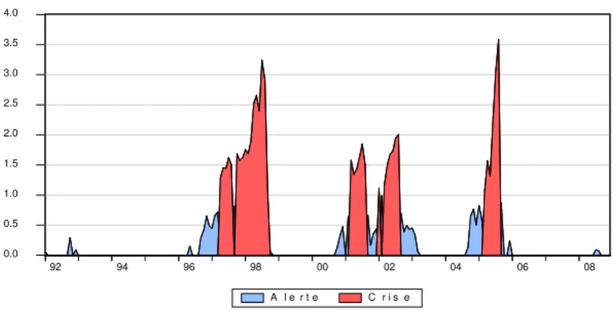
A deeper analysis shows that crises break out during the lean period and are preceded by a period of high prices that can be regarded as an alert phase. This phenomenon is most obvious in Niger: crises erupt in April and end in September; they are preceded by a period during which prices are above their trend value that runs from September/October to March. Thus, for example in Maradi, millet prices were above their trend value from September 1996 to March 1997 while the crisis broke out in April 1998 (Figure 3). At Gaya, prices were above their trend value from September 1996 to January 1997, when the crisis broke out.
Figure 3. Niger. Characteristics of crises over the period 01.1990 – 10.2008
In red: crisis phase: Iit≥1; gray: alert phase: Iit >0
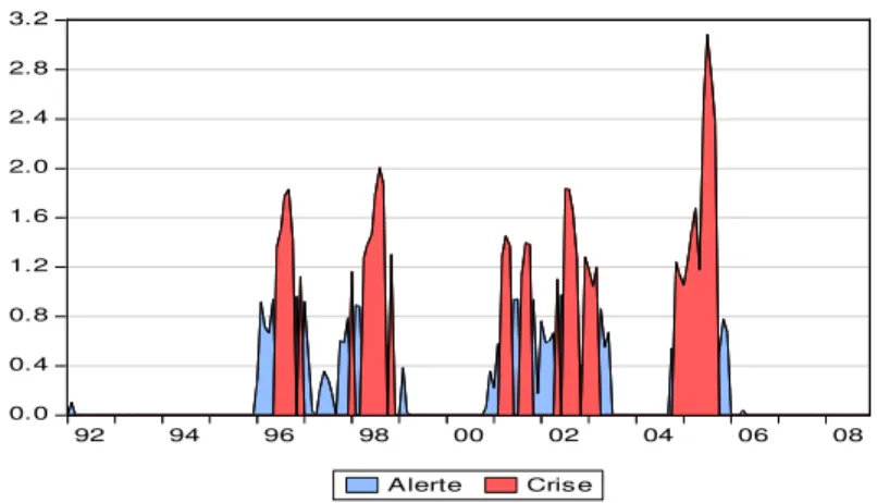
In Mali, crises occur later in the year, during May or June and end in October-November. This lag follows the harvest calendar that starts later in Mali. Phases of crises are preceded by a period of high prices running from October to May. Thus, for example, the 1996 crisis that broke out in May-June on the 17 markets of the sample was preceded by a period running from October 1995 to April 1996 during which prices in almost all the markets were above their trend value (see Figure 4 as an illustration). The 1999 crisis was preceded in all markets, except Koulikoro, by a phase of high prices that began in December 1998. The 2002 crisis, the most severe, was preceded by particularly high prices since September 2001. In contrast, the 2002 crisis started very early in the year: in October or November for most markets.
Figure 4. Mali. Alert and crisis phases over the period 02.1993 – 12.2008
0.0 0.5 1.0 1.5 2.0 2.5 3.0 92 94 96 98 00 02 04 06 08 Alerte Cris e
Marc hé du mil à Nara (Mali)
In red: crisis phase: Iit≥1; in gray: alert phase:Iit >0
In Burkina Faso, as in Mali, crises occur, generally in May or June and are preceded by positive shocks but of lower magnitude from November or December. For instance, the 1996 crisis is preceded by a period of high prices running from November 1995 in Banfora, Koudougou, Tenkodogo and Tugan, and from January 1996 in Dori, February in Sankaryare (Figure 5). 0.0 0.5 1.0 1.5 2.0 2.5 3.0 3.5 4.0 92 94 96 98 00 02 04 06 08 A le r t e C ri se M arché du m i l à M aradi (Ni ger )
Figure 5. Burkina Faso. Alert and crisis phases over the period 01.1992 – 10.2008 0.0 0.4 0.8 1.2 1.6 2.0 2.4 2.8 3.2 92 94 96 98 00 02 04 06 08 Alerte Cris e
Marc hé du mil à Dori (Burk ina Fas o)
In red: crisis phase: Iit≥1; in gray: : alert phase Iit >0
In short, over the period studied, crises break out at the beginning of the lean season and reach their climax at the end of the lean season. They are usually preceded by a warning phase, characterized by prices higher than normal during the harvest period.
4. Warning indicators
The above observations lead to propose warning indicators based on the gap between prices and their trend value during the harvest and post-harvest period running from October to March. Different indicators are proposed and their relevance is tested using nonlinear panel models.
These indicators aim at capturing as soon as possible the price movements heralding a crisis. A special attention is paid to the markets previously identified as leading markets. Three types of indicators are proposed designed to capture the intensity and the spatial extent of the shocks during the alert phase.
First, for each leading market (l), we define a binary warning indicator (IAlr) equal to
one if the market registers a positive shock during the month r, and equal to 0 otherwise. r = 1 to 6, represents the six months of the harvest period running from October to March.
IAlr = 1 if Ilr = Plr−Pˆ >lr 0 ; = 0 otherwise (4)
Ilr is the price shock on the leading market l during month r
Second, vigilance should increase with the magnitude of the price disequilibrium that is captured by an indicator of the intensity of the alert:
I lr lr I
II = /
σ
(5)This indicator is calculated for each leading market and each month (r) of the alert period (October to March).
Third, the alert should go up if many markets are simultaneously in a crisis situation. An indicator of the spatial extent of the alert is given by the number of markets on alert during the month r in the country n:
∑
= = m i ir nr IA IE 1; m = number of markets in country n. (6)
Four limitations of these warning indicators must be underlined. First, while most of the crises are preceded by an alert phase, all phases of alert do not lead to a crisis. Thus, in 1990, 1991 and 2003 in Niger, prices are above their trend value over the period September to December but the bubble bursts in March or April of next year (Figure 3). In general, it is observed that, after an alert phase, the crisis occurs or the bubble bursts in March or April. In the latter case, the alert can be lifted by March or April.
Second, the alert phase can sometimes be short and crises poorly anticipated. This is the case in 2001 in Niger: the crisis occurred suddenly in Gaya in April 2001 as well as in N'Guigmi without being preceded by an alert phase. In this case, however, the alert could be given in September at Maradi. In Burkina Faso also, the 2001 crisis broke out suddenly in March / April 2001 without a generalized warning phase. We note however, that Dori, a market identified as leader in the above analysis was on alert since November 2001.
Third, after a crisis prices return to normal level but the process may take time so that predicting prices for the following year may be difficult: prices tend to return slowly to their trend value after a crisis so that the alert holds, sometimes unnecessarily, until May / June of next year. This is the case, for example, in Mali after the 1996 crisis (Figure 4). Prices in all the markets of the sample were above their trend value until spring 1997 so that the warning indicators would be activated until April / May 1997. Similarly, after the 1998 crisis, the markets remained on alert until May / June of the following year. However, after two consecutive years of crisis in 2002 and 2003, prices returned to normal levels with the arrival of the new harvest in September 2003; the alert could then be lifted.
Finally, some markets such as Kayes and N'Guimi exhibit atypical behavior. In Kayes, crises tend to erupt later (July-August) than in other Malian markets and prices revert more slowly to their long-run equilibrium. Fluctuations in market prices of N'Guimi are also out of sync with other markets. This phenomenon can be explained by the relative isolation of these two markets compared to other markets in the sample.
5. Predictive power of early warning indicators
The predictive value of early warning indicators defined above is tested econometrically using three types of nonlinear panel models: a probit model, a count data model and a Tobit model7. Each model allows for time specific random effects.8 The sample set consists of the three countries and 19 years of time series observations (1990 – 2008).
7
See Cameron and Trivedi (2005) and Wooldridge (2001) for a review of these models. 8
A qualitative response model with fixed effects is confronted to the incidental parameters problem. In a fixed effects model the specific effects may be correlated with the regressors generally leading to inconsistent estimation of all parameters (Lancaster, 2000).
1. The first model (probit) seeks to explain the likelihood of a price crisis in country n at year t. The outcome, ynt, is a binary variable that takes 1 if the country is in crisis at year t,
and 0 otherwise. We consider that the country n is in crisis at year t if the mean crisis indicator, E(I), calculated on the sample of the m markets of the country during the lean period (s) of year t, is greater than one (Table 2). Let:
− = = ) 1 y probabilit with ( 0 ) y probabilit with ( 1 p y p y nt nt
A regression model is formed by parametrizing the probability p to depend on a regressor vector of warning indicator (x), a parameter vector
β
and time-specific effects. The conditional probability is given by:[
1 , ,]
Pr[
0]
Pr[
0]
Pr = = ∗ > = ′ + > nt nt nt t nt nt x y x u yβ
α
β
with, unt =α
t+ε
nty*: latent variable, n denotes the n-th country, t denotes the t-th time period;
α
t capture the time-specific unobserved effects assumed to be constant over individuals,(
2)
, 0
~ σα
αt iid ; εnt, is an idiosyncratic error satisfying the usual assumptions:
(
)
2
, 0
~ σε
εnt iid ,
E(xnt, εnt) = 0 and Cov (εnt , εn’t’) = V(εnt) = 1, if n = n’ and t = t’ , or 0 otherwise. The
unobservable time-specific effects are uncorrelated neither with errors nor each explanatory variable: E(αt , εnt) = E(αt , εnt’) = E(xnt, αt) = 0 (∀ n, t, t’) and Cov (αt , αt’) = V(αt) = σ²α , if t
= t’, or 0 otherwise.
The random effects MLE of β, σα² maximises the log-likelihood
(
2)
1 , , ln t t β σα N n x y f
∑
= where:(
)
∫
∞(
)
∞ − − = t t t t t t t x f y x d y f α σ α πσ β α σ β α α α 2 2 2 2 2 exp 2 1 , , , , and(
)
∏
(
)
(
)
= − ′ + Φ − ′ + Φ = N n y nt t y nt t t t t nt nt x x x y f 1 1 1 ,,α β α β α β ; Φ is the standard normal
cumulative distribution function.
The proportion of the total variance contributed by the time-level variance component is given by: 1 2 2 + = α α σ σ
ρ . When ρ is zero, the time-level variance component is unimportant and the panel estimator is not different from the pooled estimator.
2. The second estimated model is a count data model that seeks to explain the extent of the crisis. The dependent variable, ynt, is a count of the number of markets across country n
which experienced at least one episode of crisis during the lean season of the year t (Table 2). ynt, takes on nonnegative integer values, including zero: {0, 1, 2, …}.
The basic Poisson probability specification is:
(
)
(
)
! Prob y e x y f x y y
λ
λ − = = , where y! is y factorial ; λ≡E( )
yx =V( )
yx .According to Hausman and al. (1984), we consider the random effects panel Poisson specification where the Poisson parameter is specified as:~ = = ′ + , ~ >0
nt x t nt nt t nt e λ α λ λ β µ ; t e t µ
α = are the time-specific effects (unobserved); xnt is a vector of warning indicators.
Assuming that αt is distributed as a gamma random variable: αt ~ Γ(η,η), with E(αt) =
1,V(αt) = δ = 1/η and density g
(
α
tη
)
=η
ηα
tη−e−αtη Γ( )
η
1
, the Poisson model becomes:
(
)
(
)
(
)
( )
η
η
λ
η
λ
η
λ
η
η Γ + Γ × + × =∑
∑
∑
∏
−∑ y n nt n nt n nt n nt y nt nt nt y y x y f n nt nt ! ,Note that when δ is zero the panel estimator is not different from the pooled estimator.
3. The third model to be estimated is a limited dependent variable model (standard censored Tobit) that seeks to explain the intensity of the crisis (Table 2) ynt ∈ [0 ; +∞[
The censored regression Tobit model expresses the observed response, ynt, in terms of
an underlying latent variable ynt* =xnt′ β+unt
with = > = therwise o y y if y y nt nt nt nt 0 0 * * ; t = 1990, …, T ; n = 1, …, N .
xnt is a vector of warning indicators; β is a vector of parameters to be estimated; unt is a
random variable, unt =αt +εnt, defined as above.
The random effects MLE of β, σε², σα² maximises the log-likelihood
(
2 2)
1 , , , ln t t β σε σα N n x y f∑
= where:(
)
(
)
t t t t t t t x f y x d y f α σ α πσ σ β α σ σ β α α ε α ε 2 2 2 2 2 2 2 exp 2 1 , , , , , , − =∫
∞ ∞ − and(
)
∏
= − − ′ Φ − − − ′ = N n d nt t d nt t nt t t t nt nt x x y x y f 1 1 2 1 1 , , , ε ε ε εσ
β
α
σ
β
α
φ
σ
σ
β
α
dnt = 1 if y*nt > 0 ; 0 otherwise; φ(.) and Φ(.) : respectively, standard normal probability and
cumulative distribution function.
The independent variables in the probit, tobit and count models are the warning indicators defined above: a binary warning indicator for each leading markets (IAlr), an
indicator of the alert intensity for each leading markets (IIlr), and the number of markets on
alert (IEnr). These three types of indicators are calculated monthly on the harvest and post-harvest period from October to March.
Table 3. Probit model. Dependent variable = 1 if the country is in crisis; = 0 otherwise (1) (2) (3) (4) (5) (6) (7) (8) (9) (10) (11) Constante -3.497 (1.575)** -3.414 (1.173)*** - 3.606 (1.467)*** - 3.668 (1.46)*** - 2.855 (1.235)** - 3.308 (1.239)*** - 4.030 (1.342)*** - 4.255 (1.271)*** - 4.524 (1.527)*** - 5.505 (2.824)** - 3.232 (1.489)** Maradi November (Niger) 3.643 (1.797)** Gaya November (Niger) 2.965 (1.678)* Dori November (Mali) 3.606 (1.780)** Tenkodogo November (Burkina Faso) 3.257 (1.739)* A le rt a t le ad in g m ar k et Nara December (Mali) 2.855 (1.827)* November 0.168 (0.101)* December 0.261 (0.112)** January 0.265 (0.106)*** February 0.322 (0.119)*** N u m b er o f m ar k et s o n al er t March 0.430 (0.211)** Maradi November 6.257 (3.327)* Ia m l Log-likelihood - 17.476 -19.446 - 17.677 - 18.439 - 18.479 - 19.340 - 17.474 - 17.505 - 15.382 - 12.885 - 15.954 σα 2.029 (1.017) 2.779 (1.154) 2.352 (1.061) 2.565 (1.136) 2.714 (1.255) 2.977 (1.384) 2.853 (1.290) 2.900 (1.226) 2.481 (1.122) 2.005 (1.340) 1.885 (0.980) ρ 0.805 (0.158) 0.885 (0.084) 0.847 (0.117) 0.868 (0.101) 0.880 (0.097) 0.899 (0.085) 0.891 (0.088) 0.894 (0.080) 0.860 (0.109) 0.801 (0.213) 0.780 (0.178) LR (ρ = 0) 8.43 [0.002] 13.73 [0.000] 11.68 [0.000] 13.42 [0.000] 13.87 [0.000] 13.93 [0.000] 12.32 [0.000] 12.89 [0.000] 9.75 [0.001] 5.47 [0.010] 7.42 [0.003] Nb of observations 51 51 48 48 45 49 49 52 52 52 51
Significance level: * 10%, ** 5%,*** 1%. Standard errors are in parenthesis; p-value are in brackets. Approximation method of the log-likelihood: adaptive Gauss-Hermite quadrature (Naylor – Smith, 1982) ; Iaml : intensity of the alert on the leading markets.
The test strategy consists in introducing successively the monthly warning indicators in the regressions, starting with the earliest indicator (October) and ending with the last one (March). The testing procedure stops when the indicator enters significantly in the regression. This procedure allows both testing the adequacy of warning indicators and identifying those that detect the earliest a looming crisis.
The estimation results for the probit model are given in Table 3; Table 4 gives the marginal effects of the exogenous variables. The share of the specific component (
ρ
) is quite high and significant which means that the panel estimation is more relevant than the pooling estimation (see the likelihood ratio test).The warning indicator for the leading market Maradi is significant from November (Table 3, column 1) and its marginal effect on the probability of crisis is 56% (Table 4). According to these results, if the millet price in Maradi is above its trend value during November, the likelihood of a generalized crisis arising 6 to 7 months later is 56%. The probability of crisis also increases by, respectively, 33%, 50% and 34%, if the markets of Gaya, Dori, and Tenkodogo (three leading markets) are on alert in November. However, an alert at Nara may not be considered as a significant harbinger of a crisis until December. Table 4. Marginal effects: probability of a price crisis (probit model)
Maradi November Gaya November Dori November Tenkodogo November Nara December Market on alert (IAls)
0.558 0.326 0.500 0.340 0.498
November December January February March
Number of markets on alert
(IEns) 0.067 0.104 0.106 0.128 0.172
November Alert intensity at Maradi (IIls)
0.736 Source: the authors.
Therefore, the marginal effect of an alert in Maradi during the month of November is high in both absolute terms and relative to the marginal effect of an alert in any other of the leading markets considered. These results confirm the importance of monitoring the price movements in Maradi.
The variable "number of markets on alert" is also significant from November (Table 3, columns 6-10). The marginal effect of the number of markets on alert in November on the probability of crisis is 7% and this effect increases over time: it increases to 10, 11, 13 and 17% from December to March.
The alert intensity which is measured as the price deviation to its trend value relative to its standard deviation appears to be a good indicator of the occurrence of a crisis. This indicator is more relevant than the scope of the alert which is caught by the number of markets on alert. Indeed, the marginal effect of the alert intensity at Maradi on the probability of crisis is as high as 74% for the month of November (Table 4). In other words, the higher the price shocks in Maradi at the beginning of the season, the greater the likelihood of a widespread crisis.
In the count data model, the incidence rate ratio (IRR) is given by eβ; it measures the variation in the dependant variable for a one unit change in the independent variable, xnt, with
The results from this model (Table 5) confirm the previous ones. The warning indicator of Maradi significantly explains, since November, the extent of the crisis to come. The same applies for the Dori’s warning indicator since December. Specifically, the IRR shows that when Maradi (Dori) goes on alert in November (December) the predicted number of markets in crisis increases by a factor of 6.725 (Equations 1 and 3, Table 5). We note that an alert in Gaya or Tenkodogo in November or December does not significantly predict the extent of the crisis (equations 2 and 4, Table 5). Lastly, the LR test confirms that the panel estimator is more relevant than the pooling estimator.
The number of markets on alert (equations 5-9, Table 5) enters significantly in the Poisson regression model but its ability to predict the extent of the crisis is rather low, with an IRR close to one in November. However the IRR for the number of markets on alert in March is slightly higher: the expected number of market in crisis increases by 17% when one more market is on alert during March.
The intensity of the alert on the leading markets, especially Maradi, is only significant from February, and cannot be considered as a good predictor of the extent of the crisis (equations 10-13, Table 5). In other words, the number of markets affected by the crisis is not directly related to the magnitude of price shocks in Maradi at the beginning of the season.
The results from the Tobit model (Table 5) corroborate the previous ones: the warning indicator for Maradi in November is positively related to the intensity of the coming crisis. The same applies for the Gaya’s warning indicator in November as well as Dori and Tenkodogo in December. The marginal effects9 show that when Maradi goes on alert in November, the crisis intensity rises by 2.8. The marginal effect of the Dori’s warning indicator (November) and Tenkodogo (December) is of the same order of magnitude; it is lower for Gaya (November) (equations 14-17, Table 5).
As in the probit model case, the marginal effect of the number of markets on alert increases with time (equations 18 to 22, Table 5). Finally, the intensity of the alert at Maradi at the beginning of the season (November) significantly explains the intensity of the future crises. However, the marginal effect of this variable on the intensity of the crisis is not higher than the effect of the binary warning indicator.
9
Marginal effect on the expected value for y is given by:
Φ = ∂ ∂
σ
β
i X x y E[ ]. This indicates how a one unit change in an independent variable x affects censored observation (y).
Table 5. Estimation results for the count data model and the censured data Tobit model
Count data model (Poisson) Censured data Model (Tobit)
Dependent variable Number of markets that have experienced at least one episode of
crisis during the lean season Crisis intensity
Variables explicatives β IRR δ LR (δ=0) Log-V Eq. β marginal
effect σα ρ Log-V Eq. obs Maradi November (Niger) 1.906 (0.875)** 6.725 (5.884)** 3.255 (1.380) 152.13 [0.000] - 113.56 (1) 3.187 (1.106)*** 2.812 1.822 (0.505) 0.719 (0.130) - 52.87 (14) 51 Gaya November (Niger) 1.109 (0.962) 3.032 (2.917) 4.018 (1.612) 248.58 [0.000] - 117.84 (2) 2.285 (1.196)** 1.792 2.135 (0.580) 0.781 (0.106) - 55.18 (15) 51 Dori December (Mali) 1.915 (0.913)** 6.786 (6.195)** 3.152 (1.408) 154.80 [0.000] - 110.64 (3) 3.182 (1.197)*** 2.792 1.922 (0.553) 0.739 (0.126) - 50.88 (16) 48 A le rt a t le ad in g m ar k et Tenkodogo december (Burkina Faso) 1.420 (0.976) 4.136 (4.037) 3.697 (1.593) 219.95 [0.000] - 111.49 (4) 3.453 (1.273)*** 3.151 1.932 (0.551) 0.739 (.126) - 50.45 (17) 48 November 0.034 (0.019)* 1.035 (0.019)* 4.053 (1.625) 241.75 [0.000] - 113.50 (5) 0.117 (0.054)** 0.117 2.131 (0.566) 0.806 (0.098) - 54.47 (18) 49 December 0.066 (0.020)*** 1.068 (0.022)*** 3.747 (1.535) 206.46 [0.000] - 109.95 (6) 0.170 (0.051)*** 0.170 1.975 (0.513) 0.815 (0.095) - 52.06 (19) 49 January 0.087 (0.022)*** 1.091 (0.025)*** 4.042 (1.650) 218.95 [0.000] - 108.28 (7) 0.192 (0.049)*** 0.192 2.061 (0.528) 0.848 (0.081) - 51.43 (20) 52 February 0.122 (0.024)*** 1.129 (0.027)*** 3.442 (1.473) 162.84 [0.000] - 101.74 (8) 0.214 (0.043)*** 0.214 1.831 (0.462) 0.847 (0.082) - 48.10 (21) 52 N u m b er o f m ar k et s o n al er t March 0.159 (0.028)*** 1.173 (0.033)*** 2.321 (1.164) 78.03 [0.000] - 97.43 (9) 0.253 (0.044)*** 0.253 1.460 (0.369) 0.789 (0.106) - 44.49 (22) 52 Maradi November 2.367 (1.557) 10.670 (16.611) 3.473 (1.443) 204.93 [0.000] - 113.93 (10) 3.793 (1.123)*** 3.096 1.885 (0.980) 0.676 (0.140) - 52.05 (23) 51 Maradi December 2.581 (1.741) 13.214 (23.011) 3.516 (1.455) 218.59 [0.000] - 113.99 (11) 3.691 (1.230)*** 2.906 1.732 (0.486) 0.706 (0.132) - 53.03 (24) 51 Maradi January 1.569 (1.023) 4.807 (4.920) 3.786 (1.567) 186.30 [0.000] - 114.69 (12) 3.269 (0.872)*** 2.812 1.485 (0.435) 0.640 (0.151) - 51.80 (25) 52 A le rt i n te n si ty Maradi February 2.450 (1.191)** 11.592 (13.81)** 3.233 (1.393) 168.85 [0.000] - 113.75 (13) 3.640 (0.935)*** 3.169 1.448 (0.419) 0.626 (0.154) - 51.10 (26) 52 Significance level: * 10%, ** 5%,*** 1%. Standard errors are in parenthesis; p-value are in brackets. IRR : Incidence rate ratio.
To sum up, the results show that the three types of warning indicators identified above, are relevant as they significantly explain the scope and the intensity of future crises. Our analysis shows that it is of most importance to monitor millet price movements in Maradi during the harvest period. Indeed, the probability of a generalized crisis bursting 5 to 6 months later sharply increases when prices in Maradi are above their trend value in November. The results also show that monitoring all markets during the harvest period does not bring significant additional information. However, it may be useful to monitor, in addition to Maradi, the markets of Gaya, Nara and Tenkogogo: if these markets are also on alert during the last months of the year, the probability of crisis increases significantly.
6. Conclusion
Whatever the explanatory factors of the price crisis, our analysis shows that it is possible to anticipate crises from the observation of past price movements. The crises that erupt usually during April or May, may in fact be anticipated as early as in November monitoring the price movements in some key markets: Maradi first, but also Dori, and to a lesser extent Gaya and Tenkodogo.
The warning indicators defined in this paper should usefully complement the early warning systems currently focused on crop monitoring. They have the advantage of being based on objective information, easy to collect and which treatment could be rapid. These indicators can be calculated in each country and integrated into the national warning device. However, the high correlation of crises should encourage the construction of a regional warning system, incorporating indicators coming from the three countries. Irregularities detected early, at the beginning of the harvest, on the border markets of Nigeria and Benin must lead to alert not only the authorities of Niger but also of Burkina Faso and Mali of the possible occurrence of a crisis.
Of course, our calculations face a number of limitations. The main one is the quality of the estimated price trend value. We used a very simple form for the trend equation. The advantage of this specification is ease of calculation and updating of indicators. In return, the goodness of fit is sometimes poor. The introduction of the consumer prices index instead of the trend variable generally improves the accuracy of the estimates. However the consumer prices index is published with a delay of several months, so a warning system based on this index would be ineffective.
Ex post, the adequacy of the warning indicators, based on the price deviation from their trend value seems to be satisfactory but it is difficult to assess the ability of these indicators to prevent crises ex ante. Simulations were made for the period 2000-2008 which were satisfactory (Araujo Bonjean and Brunelin, 2010). They show, however, the need to periodically update the price trend. In that purpose, we suggest a “conservative” approach that consists in updating the trend estimates only if the predicted trend values are lower than previous forecasts. This method that tends to underestimate the trend value is expected to lead to a better detection of the coming crises although at the cost of an increase in the number of false alarms.
Bibliographie
Aker J. (2010), « Chocs pluviométriques, marchés et crises alimentaires : l’effet de la sécheresse sur les marchés céréaliers au Niger », Revue d’Economie du Développement, (1), March pp. 71-108.
Araujo Bonjean C. and S. Brunelin (2010), « Prévenir les crises alimentaires au Sahel : des indicateurs basés sur les prix de marchés », Document de travail, n°95, AFD, may.
Araujo Bonjean C, J. Egg and M. Aubert (2008) « Commerce du mil en Afrique de l’Ouest : Les frontières abolies ? », Etudes et Documents, n°31, CERDI.
Araujo Bonjean C. and J.-L. Combes (2010), « De la mesure de l’intégration des marchés agricoles dans les pays en développement » Revue d’Economie du Développement, (1), March pp. 5-20.
Araujo C., C. Araujo Bonjean and J. Egg (2010), “Choc pétrolier et performance des marchés du mil au Niger”, Revue d’Economie du Développement, (1), March, pp.47-70.
Azam J.P. and Bonjean C. (1995), "La formation du prix du riz : théorie et application au cas d'Antananarivo (Madagascar)", Revue Economique, vol. 48(4), July, pp.1145-1166.
Cameron A.C. and P.K. Trivedi (2005), Microeconometrics: Methods and Applications, Cambridge University Press, New York.
Deaton A. and G. Laroque (1992), « On the behaviour of commodity prices », Review of
Economic Studies, 59, 1-23.
Egg J., D. Michiels, R. Blein et V. Alby Florès (2006), « Evaluation du dispositif de prévention et de gestion des crises alimentaires du Niger durant la crise de 2004-2005 », Main report, IRAM, Paris.
Hausman J., B. Hall & Z. Griliches (1984), “Economic models for count data with an application to the patents-R&D relationship”, Econometrica, 52, pp. 909 – 938.
Lancaster T. (2000), “The incidental parameter problem since 1948”, Journal of
Econometrics, Volume 95, Issue 2, April, pp 391-413.
Naylor J.C. & A.F.M. Smith, (1982), “Application of a method for the efficient computation of posterior distributions”, Journal of the Royal Statistical Society, series C, vol. 31(3), pp. 214 – 225.
Ravallion M. (1985), “The performance of rice markets in Bangladesh during the 1974 famine”, The Economic Journal, vol. 95(377), March, pp. 15-29
Wooldridge J.M. (2001), Econometric Analysis of Cross Section and Panel Data, The MIT Press.
Appendix
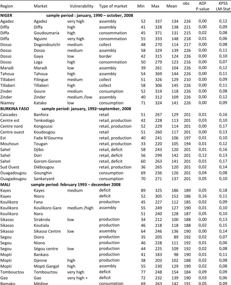
Table A1. Markets’ characteristics and unit root tests.
Region Market Vulnerability Type of market Min Max Mean obs ADF
P.value
KPSS LM-Stat
NIGER sample period : january, 1990 – october, 2008
Agadez Agadez very high assembly 52 337 134 226 0,00 0,12
Diffa Diffa high assembly 41 328 138 221 0,00 0,09
Diffa Goudoumaria high consommation 45 371 131 215 0,02 0,08
Diffa Nguimi very high consommation 55 333 148 218 0,01 0,06
Dosso Dogondoutchi medium collect 48 270 114 217 0,00 0,08
Dosso Dosso medium assembly 58 329 139 226 0,00 0,11
Dosso Gaya low border 42 315 124 226 0,00 0,10
Dosso Loga high consommation 50 279 123 216 0,00 0,07
Maradi Maradi low assembly 39 261 104 226 0,00 0,12
Tahoua Tahoua high assembly 54 369 144 226 0,00 0,11
Tillaberi Filingue medium collect 51 326 129 210 0,00 0,09
Tillaberi Tillaberi high collect 58 306 145 226 0,00 0,11
Zinder Goure medium consumption 52 319 118 226 0,00 0,08
Zinder Zinder medium /low assembly 40 312 109 226 0,00 0,12
Niamey Katako low consumption 71 324 141 226 0,00 0,09
BURKINA FASO sample period: january, 1992–september, 2008
Cascades Banfora retail 51 267 129 201 0,01 0,16
Centre est Tenkodogo retail, production 42 228 113 201 0,03 0,10
Centre nord Kongoussi retail, production 52 229 114 201 0,00 0,17
Centre ouest Koudougou retail 51 260 117 201 0,00 0,13
Est Fada N'Gourma retail, production 40 241 106 197 0,01 0,10
Mouhoun Tougan retail, production 33 220 105 194 0,01 0,12
Sahel Djibo retail, deficit 58 243 120 201 0,01 0,16
Sahel Dori retail, deficit 56 299 142 201 0,12 0,13
Sahel Gorom-Gorom retail, deficit 60 263 141 201 0,01 0,17
Sud Ouest Diébougou retail, production 36 265 120 201 0,02 0,14
Ouagadougou Gounghin consumption 69 236 126 201 0,04 0,08
Ouagadougou Sankaryaré consumption 70 271 137 201 0,05 0,10
MALI sample period: february 1993 – december 2008
Kayes Kayes medium deficit 89 325 186 189 0,05 0,18
Kayes Nioro deficit 52 305 152 186 0,16 0,11
Koulikoro Fana production 45 227 112 185 0,02 0,09
Koulikoro Koulikoro Gare medium /high assembly 55 249 127 190 0,01 0,10
Koulikoro Nara 51 240 128 187 0,05 0,10
Sikasso Sirakrola low production 34 212 100 188 0,00 0,13
Sikasso Koutiala production 46 218 118 188 0,02 0,15
Sikasso Sikasso Centre low assembly 64 246 136 190 0,00 0,14
Segou Dioro production 35 205 89 192 0,02 0,07
Segou Niono production 46 228 111 192 0,01 0,06
Segou Ségou centre low production 44 225 109 192 0,02 0,08
Mopti Bankass production 41 183 98 190 0,01 0,11
Mopti Djenne high production 38 203 102 188 0,02 0,08
Mopti Mopti Gangal high assembly 55 230 129 190 0,02 0,08
Tombouctou Tombouctou very high deficit 77 248 154 184 0,09 0,09
Gao Gao very high + deficit 72 232 139 190 0,03 0,06
Bamako Médine consumption 69 263 142 191 0,05 0,09
Source: SIMs and authors' calculations.