HAL Id: hal-01209007
https://hal.archives-ouvertes.fr/hal-01209007
Submitted on 5 Jun 2020
HAL is a multi-disciplinary open access archive for the deposit and dissemination of sci-entific research documents, whether they are pub-lished or not. The documents may come from teaching and research institutions in France or abroad, or from public or private research centers.
L’archive ouverte pluridisciplinaire HAL, est destinée au dépôt et à la diffusion de documents scientifiques de niveau recherche, publiés ou non, émanant des établissements d’enseignement et de recherche français ou étrangers, des laboratoires publics ou privés.
technology modeling: The case of greenhouse gas
emissions in French meat sheep farming
K Hervé Dakpo, Philippe Jeanneaux, Laure Latruffe
To cite this version:
K Hervé Dakpo, Philippe Jeanneaux, Laure Latruffe. Inclusion of undesirable outputs in production technology modeling: The case of greenhouse gas emissions in French meat sheep farming. [University works] auto-saisine. 2014, 47 p. �hal-01209007�
Inclusion of undesirable outputs in production technology
modeling: The case of greenhouse gas emissions in
French meat sheep farming
K. Hervé DAKPO, Philippe JEANNEAUX, Laure LATRUFFE
Working Paper SMART – LERECO N°14-08
December 2014
UMR INRA-Agrocampus Ouest SMART (Structures et Marchés Agricoles, Ressources et Territoires) UR INRA LERECO (Laboratoires d’Etudes et de Recherches en Economie)
Les Working Papers SMART-LERECO ont pour vocation de diffuser les recherches conduites au sein des unités SMART et LERECO dans une forme préliminaire permettant la discussion et avant publication définitive. Selon les cas, il s'agit de travaux qui ont été acceptés ou ont déjà fait l'objet d'une présentation lors d'une conférence scientifique nationale ou internationale, qui ont été soumis pour publication dans une revue académique à comité de lecture, ou encore qui constituent un chapitre d'ouvrage académique. Bien que non revus par les pairs, chaque working paper a fait l'objet d'une relecture interne par un des scientifiques de SMART ou du LERECO et par l'un des deux éditeurs de la série. Les Working Papers SMART-LERECO n'engagent cependant que leurs auteurs.
The SMART-LERECO Working Papers are meant to promote discussion by disseminating the research of the SMART and LERECO members in a preliminary form and before their final publication. They may be papers which have been accepted or already presented in a national or international scientific conference, articles which have been submitted to a peer-reviewed academic journal, or chapters of an academic book. While not peer-reviewed, each of them has been read over by one of the scientists of SMART or LERECO and by one of the two editors of the series. However, the views expressed in the SMART-LERECO Working Papers are solely those of their authors.
Inclusion of undesirable outputs in production technology modeling:
The case of greenhouse gas emissions in French meat sheep farming
K. Hervé DAKPO
INRA, UMRH, F-63122 Saint Genès-Champanelle, France IRSTEA, UMR Métafort, F-63178 Aubière, France
Philippe JEANNEAUX
VetAgro Sup, UMR Métafort, F-63370 Lempdes, France
Laure LATRUFFE
INRA, UMR1302 SMART, F-35000 Rennes, France
Acknowledgments
The authors are grateful to the Auvergne Region for funding this research. They also thank the INRA Egeé team of UMRH, Clermont-Ferrand, France, for their support.
Corresponding author Laure Latruffe
INRA, UMR SMART
4 allée Adolphe Bobierre, CS 61103 35011 Rennes cedex, France
Email: laure.latruffe@rennes.inra.fr Téléphone / Phone: +33 (0)2 23 48 53 93 Fax: +33 (0)2 23 48 53 80
Les Working Papers SMART-LERECO n’engagent que leurs auteurs.
Inclusion of undesirable outputs in production technology modeling: The case of greenhouse gas emissions in French meat sheep farming
Abstract
We consider different models that assess eco-efficiency in the perspective of production frontier estimation. These models span from the ones that consider bad outputs as inputs, or as outputs under the weak disposability assumption, or under the weak G-disposability and the materials balance principles, or under the modeling of multiple sub-technologies like the by-production model, or under the natural and managerial disposability concepts. These models are confronted to livestock farming data (meat sheep) and greenhouse gas pollution in French grassland areas, to discuss their suitability in eco-efficiency measurement. A major contribution is that we propose a new version of the by-production approach by augmenting it with ‘interdependence constraints’. Although all models considered here confirm the existence of large improvement potentials, all except the by-production model converge to the same results as in the case where undesirable outputs are treated as inputs. By contrast, the by-production model with interdependence provides more realistic results than the other models.
Keywords: eco-efficiency, bad outputs; materials balance principles, weak G-disposability,
by-production technology, natural and managerial disposability, greenhouse gas emissions, meat sheep farming
Intégration des biens indésirables dans la modélisation de la technologie de production : Le cas des émissions de gaz à effet de serre des exploitations françaises de viande ovine
Résumé
Nous faisons ici une revue des différents modèles d’évaluation de l’éco-efficience dans le cadre de l’estimation des frontières de production. Parmi ces modèles figurent, d’une part, ceux qui considèrent les biens indésirables soit comme des intrants additionnels de production, soit comme des produits mais sous l’hypothèse de faible disposition, ou sous l’hypothèse de disposition faible au sens de G, ou sur la base du principe du bilan de la matière. D’autre part, il existe également les modèles qui représentent la technologie de production comme l’intersection de multiples sous-technologies différentes, tout comme le modèle de production jointe, ou celui basé sur les concepts de disposition naturelle et managériale. Afin d’évaluer et analyser la praticité et l’adéquation de ces modèles dans la mesure de l’éco-efficience, nous les confrontons avec des données réelles d’exploitations d’élevage spécialisées dans la production de viande ovine dans le Massif Central, et de leurs émissions des gaz à effet de serre. De plus, une contribution majeure est que nous proposons une extension du modèle de production jointe en incluant une contrainte d’interdépendance entre les différentes sous-technologies. Malgré un potentiel d’amélioration des performances pour l’échantillon considéré, tous les modèles excepté celui de production jointe convergent vers les mêmes résultats lorsque les biens indésirables sont considérés comme des intrants. De plus, le modèle de production jointe avec interdépendance donne des résultats plus réalistes que les autres modèles.
Mots-clés : éco-efficience, biens indésirables, bilan de la matière, faible disposition, production
jointe, disposition naturelle et managériale, gaz à effet de serre, exploitations de viande ovine
Inclusion of undesirable outputs in production technology modeling: The case of greenhouse gas emissions in French meat sheep farming
1. Introduction
Since the creation of the Intergovernmental Panel on Climate Change (IPCC) in 1988, numerous scientific reports (see for example Pachauri and Reisinger, 2007) have alerted on the major role played by anthropogenic greenhouse gases (GHG) released in the atmosphere on global warming. The foreseen consequences may spread over all human life aspects (e.g. health, food production, water shortage, extreme climatic events such as droughts, floods and storms), and their economic costs could be outstanding (Stern, 2007). Hence, under the auspices of the United Nations, numerous countries ratified the Kyoto protocol which sets binding targets for developed countries to reduce their GHG emissions (Breidenich et al., 1998). This has stressed the importance of firms’ sustainable production behavior in mitigating climate change. In agriculture this is particularly true for the grazing livestock production sector, since it is the biggest emitter of GHG in the agricultural sector, as underlined in many reports over the last decade (e.g. Steinfeld et al., 2006; Gerber et al., 2013).
Evaluating the environmental performance of firms has then become crucial. But at the same time, economic performance should not be forgotten. It is therefore necessary to better understand how to model the tradeoffs between ‘intended outputs’ produced by firms, and detrimental environmental outcomes, also referred to as undesirable or bad or unintended outputs. An appropriate assessment of economic performance should integrate the by-production of environmental damages, in order to avoid erroneous measures (Zaim, 2004).
In performance benchmarking1, the concept of eco-efficiency which emerged in the 1990s, has been proposed as a suitable tool for linking economic value to environmental impact in a sustainability framework (Mickwitz et al., 2006). The notion is defined by the World Business Council for Sustainable Development (WBCSD) as ‘…the delivery of competitively priced goods
and services that satisfy human needs and bring quality of life, while progressively reducing
1 Benchmarking can be seen as the process of revealing firms’ inefficiencies by referencing and understanding best
ecological impacts and resource intensity throughout the life-cycle to a level at least in line with the Earth’s estimated carrying capacity’. Put in other words, eco-efficiency represents a situation
where a Decision Making Unit2 (DMU) produces more value with less environmental impacts (Huppes and Ishikawa, 2005). In light of this definition, many pollution intensity ratios of pollution per unit of output or per unit of value added, have been recommended in the literature. Some of these ratios are grounded on Life Cycle Assessment (LCA), which is a method used to quantify, and identify sources of, environmental impacts of a product or a system from ‘cradle to
grave’ (Ekvall et al., 2007). It means that these impacts are evaluated from the extraction of the
natural resources up to their elimination or disposal as waste.
In the case of agriculture, and in particular for livestock farming, where LCA is widely used and accepted (Gerber et al., 2010), many studies (Casey and Holden, 2006; Lovett et al., 2006; Garnett, 2009; De Vries and De Boer, 2010; Dalgaard et al., 2014) have used this method to evaluate the pollution intensities of the major GHG releases related to breeding systems (carbon dioxide, methane and nitrous oxide). However, the different pollution ratios (based on various functional units such as kg of product, kg of protein, kg of energy corrected product…), which can be classified in the category of Key Performance Indicators (KPI), suffer from several limits. These limits relate to the implicit assumptions of constant returns to scale, partial evaluation and the Fox’s paradox (for more details see Bogetoft, 2013). To overcome these drawbacks, several new frameworks have been developed based on the standard neoclassical microeconomic approach. Actually, the search for a single general index that can account for both good outputs and bad outputs (in terms of efficiency or productivity) gave rise to many scientific publications (Tyteca, 1996; Allen, 1999; Zhou et al., 2008) relying on the distance functions (introduced by Shephard, 1970) in production frontier theory, within the framework of Data Envelopment Analysis (DEA).
The first seminal work on productivity measurement accounting for the inclusion of undesirable outputs is by Pittman (1983), whose approach is linked with index number theory (based on Caves et al., 1982) which requires price information for undesirable outputs. As pollution is considered as a non-marketed good, it would be challenging to compute productivity indexes à la Pittman given the difficulties in estimating all the abatement costs. Since then, with the
development of activity analysis (with mathematical programming methods), a flow of formulations has been proposed especially in non-parametric frontier analysis (e.g. DEA) which can be based on quantity information only. Thus, in the literature that has followed Pittman’s proposal, many formalizations of pollution-generating technologies have emerged. For long, undesirable outputs have been treated as inputs (Cropper and Oates, 1992; Hailu and Veeman, 2001) or as outputs by either assuming weak disposability and null-jointness assumptions (Färe et
al., 1986; Färe et al., 1989; Färe et al., 2012), or by proceeding with data transformation
functions (Scheel, 2001; Seiford and Zhu, 2002). Recently, major steps have been undertaken with the suggestion of extensions to circumvent drawbacks of the previous models. Among the new appealing approaches, one can note:
i) the weak G-disposability (Hampf and Rødseth, 2014) that exploits the materials balance principles (MBP) and the laws of thermodynamics;
ii) the by-production modeling (Murty et al., 2012) that assumes that a production system cannot be represented by a single equation and uses multiple independent frontier representations (Førsund, 2008) under the cost disposability hypothesis; iii) the work by Sueyoshi and Goto (2012) who also used the multiple frontiers
modeling and proposed a unified framework based on two disposability concepts: natural disposability and managerial disposability.
The three latter formulations aim at respecting the physical laws and reflect the real nature of pollution generating technologies. To date however, there has been no discussion on the convergence or divergence of these methodologies in light of an empirical application.
The objective of this paper is then to carry on a systematic comparison of the aforementioned methods and discuss their suitability to real data in agriculture, with the specific case of livestock farms. A major contribution is also that we propose a new modeling framework. The application to the livestock sector is relevant for two reasons. Firstly, the complex interactions between agriculture and the environment can make difficult the choice of a method. Secondly, the last decade saw a growing attention at the international scale of the role played by livestock farming in the global GHG emissions. Given these two issues and a projected increase in future demand of animal products, this sector is a suitable candidate to investigate the challenge of eco-efficiency computations. In this paper, we focus on meat sheep breeding systems located in
French grassland areas. For these farms, the eco-efficiency computation, based on the DEA methodology, aims at finding the maximal attainable ratio of a good output (here meat production) on a bad output (an aggregation of the three main GHG emissions, namely carbon dioxide, methane and nitrous oxide). Following Hampf and Rødseth (2014) we propose in addition a decomposition of the performance into different potential sources of improvements.
The remainder of the paper is organized as follows. In Section 2 we expose the different developments of production frontier modeling in incorporating undesirable outputs in their analytical framework. The basis and the significant features of each model are presented. In this section we also present a brief review of applications in agriculture. Section 3 describes the data used and the empirical results obtained. Section 4 discusses the appropriateness of each approach to the farm data used and points out the challenges that still remain. Section 5 concludes.
2. Pollution-generating technologies modeling: theoretical basis 2.1. DEA basic analytical framework
The non-parametric method DEA suggested by Charnes et al. (1978) is extensively used for the evaluation of DMU performance. As opposed to the parametric paradigm (Aigner et al., 1977), DEA is not based on a specific functional form, and assumes that any departure from the production frontier is due to the presence of technical inefficiencies. Let represents a vector inputs , a vector of good outputs and the number of DMU. The production technology can be represented by its inputs set and its outputs set
(1)
We shall assume the following postulates:
L1 Convexity: if , then
.
L2 Free (strong) disposability of inputs and outputs: outputs are freely disposable if . This means that for a given vector of inputs , if is produced then can also be produced as long as . On the input side the free disposability
holds if . In other words, the strong disposability states that if any input is increased (whether proportionally or not), output does not decrease.
L3 Variable returns to scale (VRS): this is a more flexible assumption than constant returns to scale (CRS).
L4 Minimum extrapolation: is the intersection of all sets satisfying postulates L1 to L3.
Other assumptions are implicitly posited: no free lunch, inactivity, non-emptiness, closeness, bounded technology (one can refer to Färe and Grosskopf (2004) for more details regarding the standard axioms of production theory). Based on the previous postulates, technology under DEA can be represented by
(2)
where represents the vector of inputs and outputs for the DMU under evaluation and the vector of inputs and outputs of the reference set, i.e. all DMUs used to construct the frontier. Now let’s augment the production set with undesirable outputs. Let denotes a vector of bad outputs, , the production technology can be re-written as
(3)
In this framework pollution can be modeled in different ways, explained below.
2.2. Pollution as input
The supporters of modeling pollution as inputs generally argue that emissions of environmentally detrimental products can be viewed as the usage of the environment’s capacity for their disposal. Hence, considering them as inputs is likely a good way to account for the consumption of natural resources. Based on DEA, the optimal good on bad output ratio for a specific can be obtained by solving the following fractional programming problem
(4)
Model (4) is simplified to one good output and one undesirable output but could be extended to multi outputs/pollutants. By making a proper change of variables the model can be linearized (Charnes and Cooper, 1962).
2.3. Pollution as output and the weak disposability assumption
Undesirable outputs are said to be weakly disposable if (keeping good outputs freely disposable)
(5)
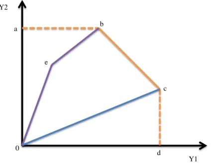
This property suggests that it is not costless to reduce bad outputs. It means that if one wishes to reduce undesirable outputs, good outputs must also be reduced for a given level of inputs. This implies that resources must be diverted to abatement activities in order to mitigate pollution level. On Figure 1 picturing a two output framework, under strong disposability of outputs the output set is represented by the segments (0abcd0). The free disposability allows some parts of the production frontier to be parallel to the axes. This does not preclude the existence of input slacks or output shortfalls (Cooper et al., 2007), also known as mix-inefficiencies. For instance, for a point lying between a and b, it is possible to improve the production of output 1 by moving toward east without worsening any other output or input. More, the existence of these slacks does
not guarantee the Pareto-Koopmans efficiency3 since some improvements are still possible. Imagine now that output Y1 is weakly disposable, then the production possibility set shifts from (0abcd0) to (0ebcd0) and the abatement intensities can be measured along the segments [0e] and
[eb]. If both outputs are weakly disposable then the new production set is (0ebc0). Figure 1: Strong and weak disposability in the production output set
Source: adapted from Färe et al. (1986)
The weak disposability assumption is generally accompanied by the null-jointness property according to which there is ‘no fire without smoke’ (Färe et al., 2007; Färe and Grosskopf, 2012) and consequently the output set contains the origin.
(6)
An optimal good and bad output ratio can be obtained by solving the fractional programming problem in (7).
3 The Pareto-Koopmans efficiency reflects a situation where, for instance, it is not possible to increase the level of
some outputs without decreasing the amount of others, or cases where it is not possible to reduce the levels of some inputs without increasing other inputs in order to maintain the same production levels.
Y1 0 Y2 a d e c b
(7)
However, as formulated in problem (7), the weak disposability assumption assumes a common proportional reduction of desirable and undesirable outputs. The model thus considers that all DMUs share the same uniform abatement effort . Yet as pointed out by Kuosmanen (2005) and Kuosmanen and Podinovski (2009) it will be wise to focus abatement activities where the abatement costs are lowest. The authors therefore proposed an extension of the traditional weak disposability assumption modeling by assuming a specific abatement effort for each producer. The new technology is similar to the one in problem (7) except that is replaced by where subscript i represents the i-th producer.
2.4. Weak G-disposability and the materials balance principles (MBP)
Before going further, let’s redefine the input variables and separate them into two sets: materials inputs (that is to say pollution-generating inputs) and non-materials inputs . The materials
balance conditions can be related to the law enunciated by Antoine Lavoisier ‘Nothing is lost,
nothing is created, and everything is transformed’. This assertion perfectly describes the first law
of thermodynamics which states that the amount of materials tied in the inputs is equal to the amount of the flow of materials embedded in the outputs plus the residuals (here denoted as
pollutants or bad outputs) (Ayres and Kneese, 1969). This law, which posits the mass conservation condition, can be represented by the mass balance equation as follows:
First law of
thermodynamics4 (8)
where are input pollution factors and is the recuperation factor of the bad output in the good one ( and are non-negative constants that evaluate the amount of environmental impact embedded in each variable category5). To be fully completed, the MBP also requires the verification of the second law of thermodynamics stated as
Second law of thermodynamics6
(9)
Based on these two laws of thermodynamics, Hampf and Rødseth (2014) proposed a new technology relating to the weak G-disposability and pollution essentiality. In addition to postulates L1, L3 and L4, this technology assumes the following:
L5 Output essentiality for the unintended outputs: ,
where represents the pollution-generating inputs.
L6 Input essentiality for the unintended outputs: . L7 Weak-G disposability of inputs and outputs:
where are direction vectors
which show the path of the disposability of the inputs and outputs. Under postulates L5 and L6 the MBP verifies the second law of thermodynamics. Inputs are no longer freely disposable, as
4
This first law is related to the mass conservation principle, and equation (8) traduces the fact that no materials are lost during the production process.
5 For example one liter of fuel generates around 3.24 kg of carbon dioxide from the extraction of the raw material to
its consumption.
6 The second law of thermodynamics simply means that there can be no residuals generated without at least some
consumption of inputs, and consequently that not all inputs are transformed into good outputs because some residuals are necessarily generated.
opposed to the weak disposability model assuming weak disposability assumption. As a matter of fact, under the weak disposability assumption, free disposability of inputs implies that for a given input bundle and a produced output set (including good and bad outputs), it is possible for a higher input bundle to produce the same amount of the output set. But this is technically infeasible under the MBP (especially for the bad outputs). The technology set can be defined as
(10)
where the direction vectors have been replaced by their empirical counterparts, the slacks S.
The optimal ratio can then be evaluated by using the following program
(11)
2.5. Pollution-generating technology modeling using by-product approach
The by-product approach, generalized by Murty et al. (2012), posits cost disposability regarding undesirable outputs and pollution-generating inputs. More precisely, the approach states that given a fixed level of inputs and intended outputs, there is a minimal amount of pollution that can be jointly-produced by the technology. Of course poor management can create some inefficiency in production that could yield more than this minimal level of undesirable outputs. Two production technology sets are constructed: an intended-production technology and a residual-generation technology. The intended-output technology satisfies standard free disposability assumptions and is independent from the level of pollution. But the intersection of these two technologies violates the free disposability assumption of both pollution-generating inputs and unintended outputs. To summarize, in by-product technology modeling there are mainly three options to reduce the levels of detrimental outputs for a fixed technology: firstly, an increase in abatement options through resource diversion (which is accompanied by a reduction of the production of good outputs); secondly, a reduction in pollution-generating inputs (this decreases the levels of intended outputs except for the case of a substitution with non-polluting inputs to maintain the same amount of good outputs production); and thirdly, the use of cleaner inputs, that is to say inputs that generate less bad outputs and maintain at least the same level of good outputs’ production. Let’s divide the input vector into two input sub-vectors where represents the sub-vector of non-polluting inputs (equivalent to ) and the sub-vector of
pollution-generating inputs (equivalent to . The general production technology can be represented by 7 (12) where (13) 8 (14)
and and are both continuously and differentiable functions. The ‘cost disposability’ assumption with respect to the unintended outputs can be expressed as follow:
(15)
The cost disposability implies that it is possible to pollute more given the levels of ; in other words it means that the set of technology is bounded below (Murty, 2010). But satisfies the standard disposability assumption:
(16)
The unified technology can be represented by (17) with two intensity variables and which represent the two different sub-technologies.
7 We can notice in equation (13) that undesirable outputs do not affect the production of good outputs in .
However, this could be generalized to allowing unintended outputs to affect the level of intended ones (pollution externality on intended outputs).
8 A rigorous modeling of technology under the materials balance conditions will imply equality in the constraint
, meaning that, given the amount of polluting inputs, the level of undesirable outputs is fixed. The model also implies that there is no recuperation factor, but this can be generalized to allow for desirable outputs to enter in the constraint. Moreover, as formulated, the model in the second technology leaves the possibility to introduce some non-linearity between polluting inputs and residual generation.
(17)
The optimal ratio can be obtained through the optimization of program (18):
(18)
The by-production approach as presented in (18) offers the advantage of disentangling the operational performance and the environmental performance. However, it assumes independence between the two frontiers and thus autonomy of the two performance measures. To overcome this
situation, we propose a new modeling approach by adding additional constraints relative to the pollution-generating inputs: (19)
Hence, by contrast to the existing literature, our contribution here is that we assume interdependence of the two frontiers. We believe that this is more likely to reflect reality since sustainability concepts are based on multiple joined objectives.
2.6. Non-radial efficiency score under natural and managerial disposability
In the same line as Murty et al. (2012), Sueyoshi et al. (2010) and Sueyoshi and Goto (2010) proposed two new unified efficiency models related to the two sub-technologies described above (respectively and ). These new models are based on two new disposability concepts attempting to unify the operational and the environmental performance into a single framework and aiming at analyzing the ‘adaptive behaviors’ of DMUs to changes in the environmental regulations:
i) The natural disposability (or negative adaptation): under this assumption, a decrease in the
vector of inputs reduces the vectors of both desirable outputs and undesirable outputs. This disposability is also termed as the ‘natural reduction’ of pollution. Under this statement, the aim of a manager would be to increase his/her operational efficiency: given a vector of reduced inputs, the firm increases the desirable outputs as much as possible. No environmental managerial effort needs to be undertaken in order to meet the objective of pollution reduction.
ii) The managerial disposability (or positive adaptation): here a firm increases the consumption
of inputs in order to increase the volume of desirable outputs and simultaneously decrease the levels of undesirable outputs. This can be achieved through some managerial effort which seeks the adoption of new technologies, such as high quality inputs or other innovative technology that can mitigate pollution. The managerial disposability concept joins the idea of Porter and Van Der Linde (1995): regulations may create the opportunity for technology innovation which may be compatible for both environment and economic prosperity.
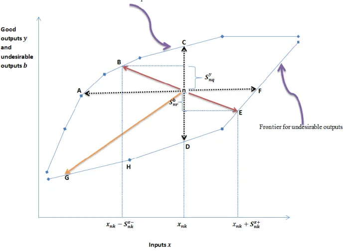
Figure 2 displays the two disposability concepts. An inefficient DMU n willing to improve its operational performance should increase its output levels and/or decrease its consumption of resources and then reach the frontier on point B. Regarding the environmental performance, two projection sides can be found on the frontier representing the bad outputs levels (the lower frontier). In the case of ‘natural’ reduction, an efficient DMU will move toward the south west of the production technology and reach point . On the contrary, an inefficient DMU n can reduce its pollution emissions simultaneously by increasing its input consumption and then reach the frontier on point E. But this input increase is only possible under ‘managerial’ effort or through the adoption of cleaner inputs. Hence, the natural and the managerial disposability concepts are both based on the orientation chosen by a producer to improve its firm’s environmental performance (along the bad outputs frontier).
Figure 2: Performance evaluation under natural and managerial disposability
Contrary to Murty et al. (2012), Sueyoshi et al. (2010) and Sueyoshi and Goto (2010) proposed a unified framework of these two disposability concepts that is based on a single intensity variable. This is possible by splitting the inputs slacks into their positive parts and their negative
parts . These inputs slacks are assumed to be mutually exclusive ( ). The optimal ratio of good output/bad output is obtained by the following mathematical programming problem: (20)
Problem (20) is augmented by the mutually exclusive constraint mentioned earlier. According to Sueyoshi and Goto (2011) two alternatives exist to estimate this model:
Add the constraint
and estimate a non-linear mathematical programming;
or,
Transform the model into a mixed integer linear programming with the following new constraints: , , where are binary for and is a very large number that needs to be defined9
.
Model (20) can be decomposed into two efficiency scores, one under natural disposability only and the other under managerial disposability. This is possible by considering the adequate slacks in the optimization10.
2.7. Eco-efficiency assessment and decomposition
In all above-mentioned fractional programming models, we have considered the maximal production intensity per unit of undesirable output. Based on these ratios an eco-efficiency score can be computed by comparing the attainable optimal ratios to the actual observed ratio. The eco-efficiency can be measured by
(21)
Based on the work of Hampf and Rødseth (2014) a decomposition of the performance score can be obtained relative to the possible choices available to the producers:
In all models presented above, we made the assumption that inputs are given and the producer does not have a free choice on these variables. By contrast, the good output and the bad output are endogenous in the estimation and the manager can freely decide their levels. Let’s denote by the optimal ratio obtained in this case.
It is possible to assume that the producer cannot freely choose nor the inputs nor the good output. Let’s denote by the optimal ratio obtained under this assumption.
A third, more flexible, possibility is to allow the free choice of the amount of inputs and of good output. This means that both variables are endogenously determined in the optimization program. Under this assumption, all DMUs converge to an optimal scale. Denote by the optimal ratio.
Based on these possibilities and the degree of adjustment offered to the producer, we can write the following relationship between the optimal ratios:
10 Under natural disposability the input constraint will only consider the negative inputs slacks (
), and under
(22)
If the eco-efficiency score is computed as , the following
decomposition can be made:
(23) The ratio
measures the eco-efficiency level when both the inputs and the good output
are held fixed. More precisely it evaluates the presence of technical inefficiencies. This measure
has been coined the ‘weak ratio efficiency’ in Hampf and Rødseth (2014). The ratio
refers
to the possible increase in the performance score when allowing flexibility regarding the level of good output. This second component has been termed the ‘allocative ratio efficiency’. The last
component of (23),
, assesses the amount by which the ratio can be improved (relative to )
when the manager can freely decide the amount of inputs. We refer to this third component as the ‘input ratio efficiency’11
. Finally, a ‘global allocative ratio efficiency’ can be obtained by multiplying the last two components of (23). It is named ‘global’ since this measure evaluates the potential improvements of the production intensity (relative to the bad output) when both the good output and the inputs can be freely allocated.
2.8. Pollution-generating technologies in agriculture: a review of the literature
Numerous studies have estimated farms’ efficiency in the presence of undesirable outputs. Most of this literature covers the generally known approaches for modeling pollution-generating technologies. As it can be seen in the studies listed in appendix, most of the existing papers deal with nitrogen pollution arising from pig production. For instance Latruffe et al. (2013) estimated the technical efficiency of Hungarian pig producers under the production of nitrogen, a
11 In fact this component compares the DMU’s eco-efficiency relative to the one of best performer in the entire
detrimental output for watershed. They assumed the strong disposability of nitrogen emissions and treated them as additional inputs. This approach has been vigorously attacked by Färe and Grosskopf (2003) and Färe and Grosskopf (2004) as it departs from the reality of the production process. In addition, assuming the strong disposability of bad outputs reflects situations where, with given quantities of inputs, one can produce unlimited amount of detrimental outputs, which is technically impossible. As a proposal to this limit, Lansink and Reinhard (2004) developed a model that still treated bad outputs as inputs, but added the weak disposability assumption of inputs which is modeled as in congestion situations (Färe and Grosskopf, 2001). On the opposite, Yang et al. (2008), considering the presence of an abatement technology, included in their model the abated amount of bad outputs as strongly disposable outputs. However, the commonly adopted approach in modeling detrimental variables as outputs is based on the weak disposability assumption. In this line, Piot-Lepetit and Le Moing (2007) considered, in pig farming systems, nitrogen surplus as outputs and assumed the weak disposability assumption of these emissions. The estimation strategy is based on the directional distance function proposed by Chung et al. (1997).
By contrast to these studies, in the light of physical laws (thermodynamics) Coelli et al. (2007) applied the MBP to the case of pig-finishing farms in Belgium. Based on the mass balance equation, the authors estimated an iso-environmental cost line the same way as a cost minimization scheme. They also demonstrated that under the weak disposability assumption, a production system might not verify the mass conservation property which the authors assume to be inherent to all materials transformation process. Yet it seems that their approach suffers from the ambiguity in the treatment of non-materials inputs12 (Hoang and Rao, 2010).
Recognizing the limits of some of the aforementioned methods (bad outputs treated as inputs; weak disposability), Asmild and Hougaard (2006) also proposed a ‘sort of data transformation’ in the case of nutrient surpluses in pig farming in Denmark. In their approach, instead of directly considering the nutrient surpluses (nitrate, potassium and phosphorous), they considered the nutrient removal by crops. Maximizing this good output (under strong disposability assumptions) indirectly reduces the nutrient surpluses. The model is set up as if the nutrient surpluses, mainly deriving from pig manure, serve as inputs to another production system (here represented by the
production of crops). The authors developed in addition several two-step approaches for the estimation of technical efficiency. For instance, in a first step one can focus on the economic efficiency (traditional technical efficieny) and thus maximize the production of good outputs (gross returns) ignoring environmental variables. In a second step one can estimate the potential nutrient removal that is possible given that the farm is economically efficient. This two-step scheme gives priority to the economic efficiency, and considers afterwards the environmental efficiency which is computed in a way that it does not create any opportunity costs or increase the economic costs of the farm13. This two-step approach can inversely be estimated by giving priority to environmental efficiency in the first step.
Another strand of approach can be found in Picazo-Tadeo et al. (2011), and is based on the estimation of the frontier eco-efficiency (Kuosmanen and Kortelainen, 2005). This model estimates a ratio of economic outcomes (represented by value added or profit) on environmental pressures. In a dual perspective, the model considers undesirable outputs as inputs and thus is subject to the criticisms previously mentioned. A recent paper of Serra et al. (2014) has explored the by-production technologies modeling in the case of crop farm systems in Spain. We have not found an application in agriculture of the natural and managerial disposability concepts, nor the weak G-disposability.
Finally, few studies in the agricultural sector have focused on the emissions of GHG. We can find in Kabata (2011) an application of the weak disposability assumption to the case of crop and livestock production in the United States, where bad outputs consist in methane and nitrous oxide emissions. Shortall and Barnes (2013) used a data transformation function (inverse) to account for the carbon dioxide, methane and nitrous oxide emissions in the case of Scottish dairy farms. Toma et al. (2013) used two different models, the weak disposability assumption and the eco-efficiency frontier estimation. Mohammadi et al. (2014) applied the approach coupling LCA to DEA, to the GHG emissions in paddy rice farms in Iran.
3. Empirical application
3.1. Data description and environmental impacts’ computations
The empirical application of the models described in the previous section is carried out on a sample of 1,261 farm-year observations between 1987 and 2012. The farms are specialized in meat sheep production and are located in the center of France in grassland areas. Several bookkeeping and production process characteristics are available in the database. Following the literature on farms’ technical efficiency, we have retained four inputs, namely utilized land, farm labor, operating expenses and structural costs. Operating expenses, also called proportional costs, comprise all costs related to animal feeding, crop fertilizers, pesticides and all the other costs directly associated to the presence of livestock (veterinary costs, mortality insurance, liter straw costs, marketing costs, animal purchase…). Regarding structural costs, they are mainly made of mechanization and building costs (depreciation, maintenance costs, expenses for fuels and lubricants, related insurances) as well as overheads (electricity, water, insurances, financial costs, opportunity costs of capital…). Operational and structural costs are expressed in constant currency (2005 Euros) to keep quantity based information. Utilized land represents the hectares available to the producer for the sheep farming activity, and labor measures the quantity of full-time workers devoted to meat sheep production. It is worth mentioning that we do not include the herd size in the inputs variables as it is the case in some studies (Karagiannis and Tzouvelekas, 2005; Ludena et al., 2005; Alvarez and Del Corral, 2010), firstly because of the evident and strong correlation with some inputs variables14. The idea is to keep a sort of independence between input variables. Secondly, an analysis with two regressions in which the dependent variable is the total amount of meat production and the independent variables are the inputs, confirms the need to exclude the herd size from the inputs. In one regression model we keep the herd size and in the second one we omit it. In the first regression the variable land has a negative sign, which is counterintuitive since this variable can be viewed as an important input in grazing livestock systems to produce meat. In the second regression (excluding herd size), we obtain reasonable results, with all the inputs exhibiting a positive and significant impact on meat production. Thirdly, the input variables describe the production process in a farm similar to a cost
14 The correlation coefficients with the other inputs are 83% for land, 74% for operational costs, and 75% for
analysis. More precisely, the costs associated to all the four aforementioned inputs (land, labor, operating costs and structural costs) simply represent the total expenses of the farming activity. Based on this idea, we argue that the variable herd size should be set aside, and used in a second stage as a determinant of the efficiency score (Latruffe et al., 2008).
On the output side, the good output is measured by the quantity of meat production expressed in kilograms (kg) of carcass, and the bad outputs relate to GHG. The computations of the latter were based on LCA methodology, which was used for the estimation of the three main GHG generally considered in livestock farming (carbon dioxide, methane and nitrous oxide). Since our interest is on global warming the three gases were summed up regarding their Global Warming Potential (GWP)15 relative to carbon dioxide. The bad output is thus the total GHG emissions expressed in carbon dioxide equivalent. When applying LCA we have restrained the system boundary (i.e. the perimeter of analysis) from the cradle to the farm gate. We adapted the GES’TIM (Gac et al., 2011) and the Dia’ terre® (Ademe, 2011) tools to our sample of meat sheep farms. These tools provide the majority of emission factors required for the estimation of the global warming impact.
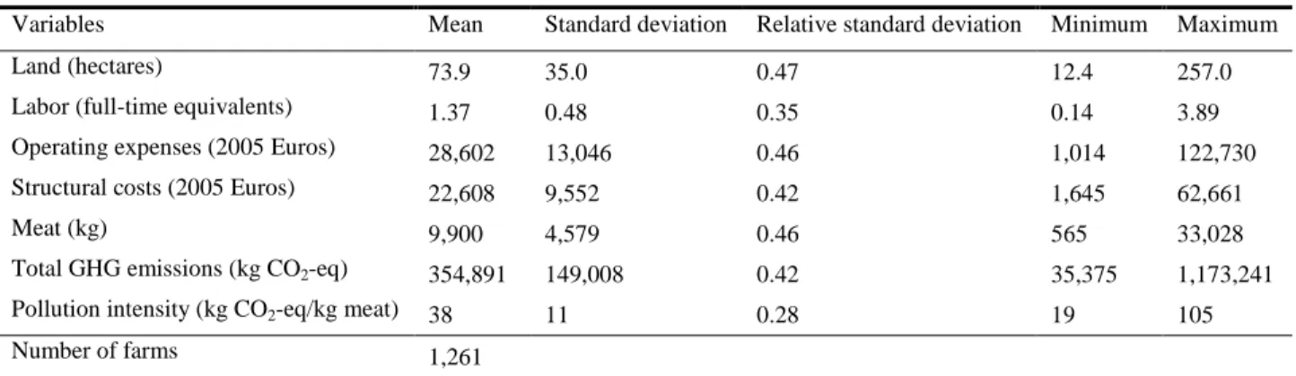
The main characteristics of the sample are summarized in Table 1. On average, over the period of study, farms in our sample produced around a thousand kg of meat carcass on a land area of 74 hectares. The pollution intensity, which is measured as the ratio of GHG emissions on meat production, is about 38 kg of carbon dioxide equivalent per kg of carcass on average. The relative standard deviation is similar for all inputs and outputs (about 0.45), except for labor and pollution per meat kg for which it is smaller (respectively 0.35 and 0.28).
15 The GWP represents the warming effect relative to carbon dioxide over a period of 100 years. It is about 25 for
Table 1: Summary statistics of the sample (period 1987-2012)
Variables Mean Standard deviation Relative standard deviation Minimum Maximum
Land (hectares) 73.9 35.0 0.47 12.4 257.0
Labor (full-time equivalents) 1.37 0.48 0.35 0.14 3.89 Operating expenses (2005 Euros) 28,602 13,046 0.46 1,014 122,730 Structural costs (2005 Euros) 22,608 9,552 0.42 1,645 62,661
Meat (kg) 9,900 4,579 0.46 565 33,028
Total GHG emissions (kg CO2-eq) 354,891 149,008 0.42 35,375 1,173,241 Pollution intensity (kg CO2-eq/kg meat) 38 11 0.28 19 105
Number of farms 1,261
Notes: CO2-eq: carbon dioxide equivalent. The relative standard deviation is computed as the ratio of the standard deviation on the mean.
3.2. Comparison of eco-efficiency from various models: empirical results
All models were applied under the VRS assumption. One single frontier was estimated for the whole period (by pooling all observations together), that it to say we assume no technological change. We consider land and labor as non-materials inputs that is to say they are assumed to generate no GHG emissions. By contrast, operating expenses and structural costs are pollution generating. The average eco-efficiencies and their components calculated with all methods described in the previous section are summarized in Table 2.
In addition to these models we have estimated two new models where we omitted the production of GHG emissions. In the first model (equation 24) we determine the potential attainable meat production given the levels of inputs.
(24)
The second model (equation 25) is based on a more flexible assumption where the producer can freely choose both the amount of inputs and good output. We then evaluate the eco-efficiency for each farm given their unchanged pollution emissions.
(25)
For the sake of simplicity we present the pollution intensity instead of the ratio of meat production per unit of GHG emission as presented in the above models. As explained above, for the approaches that include pollution in the production technology, the eco-efficiency score is based on the flexible assumption of free choice of inputs, good output and bad output.
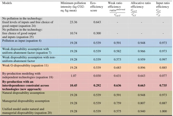
The results in Table 2 show that most of the models (pollution as input, weak disposability assumption, weak G-disposability, natural and managerial disposability, unified model under natural and managerial disposability) converge to the same eco-efficiency score (0.539 on average) and the same pollution intensity (19.28 kg CO2-eq/kg meat on average). These models
suggest that farmers can reduce 46.1% of their current pollution intensity. An interesting finding is that all these models point out the same source of inefficiency: the weak ratio efficiency appears to be the smallest, on average, among the three sources of inefficiencies. As explained earlier, this ratio accounts for the presence of technical inefficiencies in the production process since both the inputs and the good output are held fixed. However, some small differences can be found for the case of the models of weak G-disposability and managerial disposability, which give a higher score for the weak efficiency ratio compared to the other models (0.683 and 0.759 respectively). Moreover, these two models give some importance to the other sources of inefficiencies. For instance, when assuming managerial disposability, 19.3% of inefficiency arises from allocation issues (allocative ratio efficiency of 0.807) and 11.3% is related to input
management (input ratio efficiency of 0.887). In the case of the weak G-disposability model, the respective figures are 10.4% and 11.5% of inefficiency (efficiency of 0.896 and 0.885).
The most pessimistic model is the by-production modeling with independence of the two sub-technologies. In fact this model leads to ‘unrealistic’ results in terms of eco-efficiency since 97.0% of inefficiency is found to be present in the sample (eco-efficiency score of 0.030). This questionable result can be explained by the fact that the model separately optimizes the operational efficiency (with the good output frontier) and the environmental efficiency (with the bad output frontier). But when we impose an interdependence constraint, the by-production model yields more realistic results with an average eco-efficiency score of 0.292 (70.8% of inefficiency). Besides, in this latter model the three sources of inefficiency seem to play equal role in the explanation of the estimated eco-inefficiency: the weak and allocative ratios contribute to 36.4% and 33.7% (while it is 26.5% for the input ratio).
For comparison purpose, we also show the results of two variants of the technology that completely ignores the presence of undesirable outputs. In the first alternative, we have estimated the potential increase in meat production that farmers can reach on average given a fixed amount of inputs. Then we assess the eco-efficiency by using the actual values of GHG emissions. The average eco-efficiency is 64.3% with a pollution intensity of 23.36 kg CO2-eq/kg meat (first row
of Table 2). In a second alternative approach we relax the assumption of fixed levels of inputs and the producer can thus freely choose both the inputs and the good output. This new development produces an eco-efficiency score of 30.0% (first row of Table 2). This result is very close to the one obtained under by-production with interdependent sub-technologies. This reflects the fact that both approaches estimate the same thing except that in the method where pollution is not directly incorporated to the technology, the environmental efficiency score is simply set to one (and all farmers are GHG efficient). Moreover, the closeness of the values obtained from these two estimations suggests that, in the case of the producers considered in our sample, any improvement in the eco-efficiency might be undertaken by eliminating all the technical inefficiencies in the production of meat.
Table 2: Eco-efficiencies for various pollution-generating technology models: sample’s average over the period 1987-2012
Three sources of efficiency (equation 23)
Models Minimum pollution
intensity (kg CO2-eq /kg meat) Eco-efficiency score Weak ratio efficiency Allocative ratio efficiency Input ratio efficiency
No pollution in the technology: fixed levels of inputs and free choice of good output (equation 24)
23.36 0.643 - - -
No pollution in the technology: free choice of good output and inputs (equation 25)
10.74 0.300 - - -
Pollution as input (equation 4)
19.28 0.539 0.591 0.948 0.973
Weak disposability assumption with
uniform abatement factor (equation 7) 19.28 0.539 0.582 0.966 0.973 Weak disposability assumption with
non-uniform abatement factor 19.28 0.539 0.573 0.959 0.997
Weak G-disposability (equation 11)
19.28 0.539 0.683 0.896 0.885
By-production modeling with
independent technologies (equation 18) 1.07 0.030 0.631 0.643 0.077
By-production with an
interdependence constraint across technologies (new approach)
10.45 0.292 0.636 0.663 0.735
Natural disposability assumption
19.28 0.539 0.591 0.948 0.973
Managerial disposability assumption
19.28 0.539 0.759 0.807 0.887
Unified model under natural and
managerial disposability (equation 20) 19.28 0.539 0.575 0.940 1.000 Notes: CO2-eq: carbon dioxide equivalent
As earlier explained, under the flexible assumption that the producer can freely choose the levels of inputs, of good output and of bad outputs, all the DMUs converge to the same eco-efficient farm. We can then obtain the optimal scale of the operations that guarantee all farms to be eco-efficient. The results are summarized in Table 3.
All models except the by-production approach with interdependence16 and the pollution free technology produce an optimal scale where fewer inputs are used to produce more meat and emit less GHG than the actual sample average. In the case of the by-production modeling under dependent technologies, consumption of non-materials inputs (land and labor) is increased while
16 We do not consider the results obtained with the by-production approach with independent technologies given the
the pollution-generating inputs are reduced, in comparison to the sample’s average. This leads to a higher level of meat production and lower GHG emissions. It seems that with this by-production approach there is a substitution between non-materials inputs and pollution-generating ones. In implies that, with the by-production model with interdependence, farmers can produce more meat (around 10% more) than with the other pollution technologies.
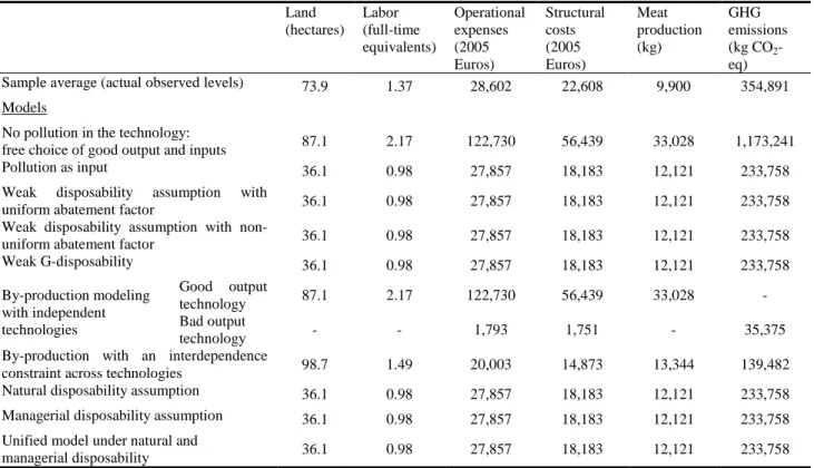
Table 3: Optimal scale for eco-efficient DMUs Land (hectares) Labor (full-time equivalents) Operational expenses (2005 Euros) Structural costs (2005 Euros) Meat production (kg) GHG emissions (kg CO2 -eq) Sample average (actual observed levels) 73.9 1.37 28,602 22,608 9,900 354,891 Models
No pollution in the technology:
free choice of good output and inputs 87.1 2.17 122,730 56,439 33,028 1,173,241 Pollution as input 36.1 0.98 27,857 18,183 12,121 233,758 Weak disposability assumption with
uniform abatement factor 36.1 0.98 27,857 18,183 12,121 233,758 Weak disposability assumption with
non-uniform abatement factor 36.1 0.98 27,857 18,183 12,121 233,758 Weak G-disposability 36.1 0.98 27,857 18,183 12,121 233,758 By-production modeling with independent technologies Good output technology 87.1 2.17 122,730 56,439 33,028 - Bad output technology - - 1,793 1,751 - 35,375
By-production with an interdependence
constraint across technologies 98.7 1.49 20,003 14,873 13,344 139,482 Natural disposability assumption 36.1 0.98 27,857 18,183 12,121 233,758 Managerial disposability assumption 36.1 0.98 27,857 18,183 12,121 233,758 Unified model under natural and
managerial disposability 36.1 0.98 27,857 18,183 12,121 233,758
However, the highest meat production is obtained under the pollution free technology where all inputs are increased to produce more than twice the amount of meat. Nevertheless, this situation creates larger levels of GHG emissions (eight times more than with the by-production with interdependence and five times more than with the other pollution technologies). The difference between pollution free technology and by-production approach with interdependence seems to be a matter of arbitrage: produce more good output to compensate for the pollution emissions (pollution free technology) or pollute less by reorganizing inputs and take advantage of the possible substitution between materials and non-materials inputs (by-production technology), and try to produce good output as much as possible given the new inputs.
4. Methodology convergence or divergence: a discussion
Although many of the presented models reach the same average optimal eco-efficiency score, they differ in their assumptions. From a theoretical perspective, models that consider pollution as input or as output under the weak disposability assumption produce arbitrary wrong tradeoffs and do not capture the real nature of undesirable outputs. Murty et al. (2012) estimated these tradeoffs and found a negative relation between pollution-generating inputs and the pollution level, which is definitely in opposition to the idea that these inputs are pollution generators. More, they also proved that under some conditions, for a fixed level of inputs there exist large possibilities of good output/bad output combinations that are efficient. This violates the idea behind by-production that there is only one minimal amount of undesirable outputs given the levels of inputs. Other shortcomings of the weak disposability assumption have been reported by Hailu and Veeman (2001) and (Chen, 2013).
To overcome the drawbacks of the previous two models (pollution as inputs and weak disposability assumption), Murty et al. (2012) developed the by-production modeling by assuming that the production process is made of different sub-technologies, and the global technology is the intersection of the good output technology and the bad output sub-technology. However, in the operationalization of the approach the authors assume independence between both frontiers. We have seen here that under this assumption inconsistent results are generated. For this reason, a contribution to the existing literature is that we propose here a new by-production modeling by introducing some interdependence constraints which link the usage of materials inputs in both frontiers. Still in relation to this multiple frontier framework, Sueyoshi and Goto (2011) proposed a unification of the operational and environmental efficiency based on the use of one single intensity factor ( ) and also by allowing two possible opposite directions for the inputs. However, in light of the previous results, this interesting approach finally collapses into the model where pollution is considered as an additional input.
The model assuming the weak G-disposability and the materials balance conditions is supposed to reflect the real production process by accounting for the laws of thermodynamics. However, in terms of results, the model also converges towards the one in which GHG emissions are treated as input. In reality when the producer can freely decide the levels of inputs, of good output and of bad output, the model becomes similar to the one where pollution is treated as input.
Finally, it is worth mentioning that, despite the fact that models which consider pollution under the weak disposability assumption, or weak G-disposability, or natural and managerial disposability, or unified model under natural and managerial disposability, converge to the same results in terms of eco-efficiency as the one where pollution is simply an additional input, some differences can be found in terms of the sources of improvements (technical inefficiencies, flexibility in output allocation, input management).
5. Conclusion
In performance benchmarking the impacts of environmental policies on firm’s efficiency have long been investigated. For this, several models of eco-efficiency calculation have been proposed to integrate and analyze the tradeoffs between intended outputs (or good outputs) and detrimental environmental outcomes (or bad outputs). In this paper we have discussed the main models developed in the literature and empirically compared eco-efficiency obtained with these models, for the specific case of meat sheep farms and GHG emissions in French grassland areas. Eco-efficiency is computed as the ratio of good output on bad output and is aimed at providing easily interpretable results. To our knowledge this is the first paper that undertakes eco-efficiency comparison in the case of livestock farming systems. Another major contribution is that we developed a new version of the by-production approach by including some dependence constraints. This model appears to provide sound results in the case of GHG emissions. In light of the obtained results, all the models come to the same conclusion of large inefficiencies present in meat sheep farms. One limitation of this study is that we did not account for carbon sequestration in soils which is a specific feature of livestock farming as a potential abatement option. This aspect could however be explicitly modeled in the by-production technology.
References
ADEME. (2011). Guide des valeurs dia’terre. Version référentiel 1.7
Aigner, D., Lovell, C., Schmidt, P. (1977). Formulation and estimation of stochastic frontier production function models. Journal of econometrics, 6(1): 21-37.
Allen, K. (1999). Dea in the ecological context—an overview. In Data envelopment analysis in
the service sector (pp. 203-235): Springer.
Alvarez, A., del Corral, J. (2010). Identifying different technologies using a latent class model: Extensive versus intensive dairy farms. European Review of Agricultural Economics,
37(2): 231-250.
Arandia, A., Aldanondo-Ochoa, A. (2011). Pollution shadow prices in conventional and organic farming: An application in a mediterranean context. Spanish Journal of Agricultural
Research, 9(2): 363-376.
Asmild, M., Hougaard, J. L. (2006). Economic versus environmental improvement potentials of danish pig farms. Agricultural Economics, 35(2): 171-181.
Ayres, R. U., Kneese, A. V. (1969). Production, consumption, and externalities. The American
Economic Review, 59(3): 282-297.
Ball, V. E., Fare, R., Grosskopf, S., Nehring, R. (2001). Productivity of the us agricultural sector: The case of undesirable outputs. In New developments in productivity analysis (pp. 541-586): University of Chicago Press.
Ball, V. E., Lovell, C. K., Luu, H., Nehring, R. (2004). Incorporating environmental impacts in the measurement of agricultural productivity growth. Journal of Agricultural and
Resource Economics, 29(3): 436-460.
Beltrán-Esteve, M., Gómez-Limón, J., Picazo-Tadeo, A., Reig-Martínez, E. (2013). A metafrontier directional distance function approach to assessing eco-efficiency. Journal of
Productivity Analysis, 41(1): 69-83.
Berman, E., Bui, L. T. (2001). Environmental regulation and productivity: Evidence from oil refineries. Review of Economics and Statistics, 83(3): 498-510.
Berre, D., Boussemart, J.-P., Leleu, H., Tillard, E. (2012). Economic value of greenhouse gases and nitrogen surpluses: Society vs farmers’ valuation. European Journal of Operational
Research. 226(2): 325-331
Bogetoft, P. (2013). Performance benchmarking: Measuring and managing performance. Springer.