M. Martinez-Sanchez and R.P. Gauthier
M. Martinez-Sanchez and R.P. Gauthier
GTL Report #202
October 1990
This research was supported by NASA Marshall SFC under Contract No. NAS8-35019
(Glenn E. Wilmer, Technical Monitor).
BLADE-SCALE EFFECTS OF TIP LEAKAGE
b y
M. Martinez-Sanchez and R.P. Gauthier
MIT Gas Turbine Laboratory
ABSTRACT
The effects of blade-tip leakage in a turbine are investigated by modeling the stage as an incomplete actuator disk. It is found that the
spanwise flow redistribution due to the gap is such as to produce a uniform unloading of the blades, despite the very concentrated leakage. Partial lift retention at the blade tip is accounted for based on a leakage jet-free stream collision model which successfully predicts the roll-up of the leakage flow. The predicted efficiency loss due to the gap correlates well with experimental
1. Introduction
The effects of the finite gap at the tip of the blades of various kinds of turbomachinery has long been a topic of study, both
theoretical and experimental, motivated largely by its strong impact on stage performance. An additional motivation arises, in our case, from the role of blade-tip losses in the generation of de-stabilizing cross forces on turbine disks. The mechanism for these forces, as first
proposed by Alford(l) and Thomas(2), is depicted in Fig. 1. It is an
empirical observation that the efficiency of a turbine decreases more or less linearly with the ratio of tip gap to blade height:
H
(1)where
p
is a numerical factor of order 1-2. Re-writing in terms of the force f per unit azimuthal length,f
-fo
_
fllDEA
fjj)EI
H (2)If a turbine disk with mean gap
8
is offset by ex in the transverse Ox direction, then, measuring azimuth 0 from the point where the gap is maximum,6
(0) = 8 - ex cos 0
(3)
We can now project all forces in the OY direction, (perpendicular to the offset), to obtain fy = f cos
0
per unit length, for a total cross-forceFY
j
fy
RdO.
Using Eqs. (2) and (3),0
Fy
=ex fiDEA nRH
2 R (4)
This force is only opposed by inertia and damping forces, since the structural restoring reactions to ex would normally act along Ox. The result, if damping is insufficient, is a divergent whirling
motion. Equation (4) shows the importance of the loss factor
p
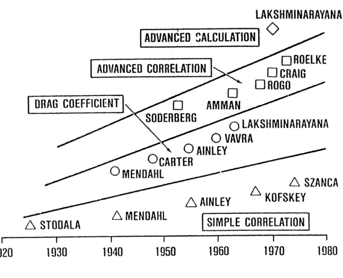
(Eq. (1)) for prediciton of the stability properties of a rotor.The extensive data base on tip-loss factors has been correlated
by many authors on the basis of various levels of analysis. A good
review of these efforts was presented by Waterman(3), from whose
paper we have borrowed Fig. 2. Waterman selected 10 well documented turbine test cases and five tip-loss prediction schemes, and obtained results which are statistically summarized in Table 1, also taken from Ref. 3. (Results based on Lakshminarayana's method were omitted because of their systematic overpredictions). Given that P averages roughly 1.5, the variances in the first column of Table 1 indicate a fairly unsatisfactory state of affairs regarding predictive capabilities. Perhaps at the root of this situation is the lack of a clear model of how the losses arise. Generally speaking, the various approaches used have fallen into three categories:
(a) Models based on calculation of the pressure-driven tip gap flow rate, plus the assumption that some portion of the kinetic energy of this flow is lost. Various corrections are used for viscous and other effects. The models of Rains(4) and Vavra(5) are in this category.
(b) Models based on adaptations of wing theory to predict the
"induced drag" produced by the trailing vorticity escaping at each blade tip. A key difficulty is the predicition of tip lift retention, which
determines the strength of such vortices. Examples are Lakshminarayana(6),(7) and Lewis and Yeung(8).
(c) More recently, detailed 2 and 3 dimensional numerical
computaions of flow in a passage, including gap effects, have become possible(9),( 1 0). While these give important insight as to many details of the flow pattern, they still lack the precision required to calculate the
regarding a much better explored problem, i.e., drag predicitions on a 2-D airfoil.
The models in Group (a) above are basically correct as to gap flow predictions, and can be regarded as a satisfactory first order description of near-gap effects. On the other hand, they ignore the concomitant small changes to the flow over the rest of the blade when a small gap is present. We will show later that it is these changes that are responsible for most of the blade force losses.
The models of Group (b), with their emphasis on induced drag, come closer to capturing the essence of the phenomenon. Indeed, the flow disturbances at the blades induced by trailing vortices can be one way of describing the blade-scale effects of tip leakage. What has been lacking is a globally consistent model of the strength and distribution of these vortices. Thus, Lakshminarayana(6) used an array of straight-line trailing vortices of uniform strength, equal to an empirically determined fraction of the blade lift. Ad-hoc corrections for vortex roll- up(7) improve the details of blade pressure distributions with little positive impact on loss prediction.
In this work, we emphasize the global nature of the blade-tip problem by using an actuator disk model for the stage. Details of the near-blade flow are in this way simplified by being relegated to the role of algebraic connecting conditions between the upstream and
downstream flows. On the other hand, the spanwise rearrangement of the flow pattern due to preferential migration towards the gap region can be correctly captured, provided one recognizes the discontinuous nature of the downstream velocity distribution (i.e., the presence of a shear layer along the tip streamsurface). This shear layer is, of course, he result of azimuthally smearing the individual "trailing vertices" of the blades. With some reasonable mathematical approximations,
results can be obtained from this model which agree with data to an equal or greater extent than existing correlations. Perhaps more
importantly, these results arc easily enough related to the basic nature
of the problem that generalization appears possible to include effects such as non-uniform gap distributions (our principal goal) or
non-uniform inlet flow. Improvements can also be introduced on the details of the flow on the gap scale to account for partial tip loading, as will be discussed.
2. FORMULATION
For maximum simplicity, our initial model will make the following assumptions, some of which will be later relaxed: (a) Imcompressible, inviscid flow
(b) Two-dimensional geometry
(c) Uniformity along the tangential (y) direction
(d) Fluid passing through the rotor blade-tip gap does no work. (c) Stage collapsed in the axial directon to a single plane, and smeared in the azimuthal direction.
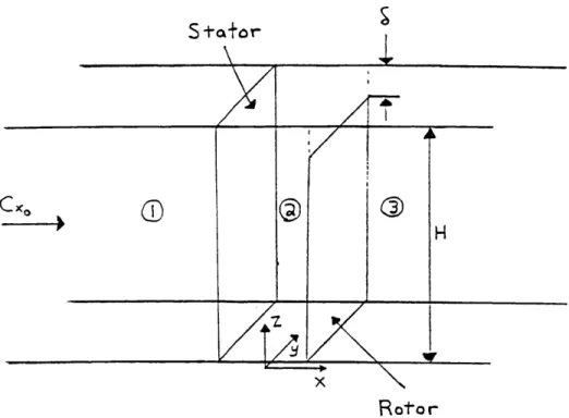
The "actuator disk" which represents the stage consists of a full-span stator and a partial-full-span rotor (Fig. 3), both occupying the x = o plane. Since there are no variations with y, the azimuthal momentum equation reads
acy acy
Cx +
C0-ax az (5a)
or, introducing the vector c1 = Icx + kcz to represent the meridional
velocity projection,
C1 .V Cy =0 (5b)
showing that C1 is simply convected by Cy. Similarly, the vorticity
equation reduces in this case to
C1.V y =0 (6)
where
Y x aCz
c1. VB Io (8) where
B,= + ic2
p 2 (9)
Continuity is satisfied by introducing the stream function P(x,z) for the meridional flow:
IIx= ;
7cz=--)z ax (IOa,b)
and then Eqs. (5b), (6) and (8) reduce to
Cy = Cy (1) (11)
Wy= 0y (") (12)
B1 = BI (') (13)
Using in Eq. (12), the definitions in Eqs. (7) and (10) produce the equation which governs P(x,z):
V2' = y(OY,) (14)
2 2 a2 D2
where, in this case, a2 a
Notice that the meridional flow (cx,cz) is decoupled from cy, and can be solved for first. The component Cy, as well as
acy acy
x- z = - , can be found a-posteriori.
Upstream of the stage (x < o), we assume the flow is irrotational
(oy
= o), and - simply obeys Laplace's equation. Uneven work extraction as the flow goes through the stage gives rise to non-zero vorticity (10y downstream of the disk, and the value of (Oy is carriedunchanged on each streamline from here on.
The vorticity (0 y and the meridional Bernoulli constant, B, are related to each other in a simple way. Starting from the Lamb form of the meridional momentum equation,
and taking the cross-product with Cj,
=-1x
VB
1C1 (15)
Remembering that, B1 = B1 (P)we have VB1 = (B VW, and
(dV
L
VB1)y =(B)
(' x VP)y. From the definition of T (Eq. 10),x V')y = - CI, so that
Wy =~j
(16)
This relationship opens the way for a connection between the downstream COy and the non-uniformity of extracted work at the disk.
Let subscripts I and 3 denote stations just upstream and just downstream of the stage (Fig. 3). Them because of continuity,
CX3= CX1 (17)
and, since we assume spanwise uniform blading, which can exert no forces on the flow in the z-direction,
CZ3= CZI (18)
Because of (17), (18) and the definition (9),
B1- B3,= PI - P3
P (19)
dB1I
-Now, upstream of the stage, the absence of vorticity implies dP and so, from (16),
_ dB 1 3 d(B -B 1 3) __ -_
d' d' d( P (20)
which gives the vorticity (0y when the distribution of (isentropic)
gives for the stagnation enthalpy decrease across the stage
- Aht = U cxtan
a
2 - (U - cx tan P3)] (21)where U is the wheel speed.
Adding to this the kinetic energy increase
A (K.E.) = 1 c23 =L (U - c, tan P3)2
2 Y3 2 (22)
we obtain, for any streamline which crosses the disk in the region covered by the blades (not the gap)
(Pi
- P3~BL
= U x tana
2-
-I (U2 - c2 tan213)
p 2 (23)
Exactly how much work is extracted from those streamlines which at some point cross the blade-tip gap is a relatively complicated question to answer, and to which we will return in Sections 8,9. For now, we will make the simplest possible approximation, namely, that no work is extracted. This implies for such streamlines
(
3GAP 1P - P2 Lc Ctan2 a 2P p 2 (24)
In Eqs. (23), (24), the axial velocity cx at the disk is to be regarded as a function of z, in anticipation of redistribution of the flow in
response to the presence of the gap. When using Eqs. (20), therefore, we will put
dx icx az a' x =0 o x az x =0 acx
BLADES: C)y = -
[
-
tan a2 + tan2P3
(CX
'(C,
x=0 az x=O (25a)
GAP: y = tan2U2 az
aSz
Jx=o
= (25b)Since there is a discontinuity in the connecting conditions for flow through the gap versus flow through the blade passages, we can also expect a discontinuity, in the form of a shear layer, on the
downstream portion of the streamline which passes through the blade ips. Denoting by superscripts (+) and (-) the regions on the gap and blade side of this layer, respectively, (Fig. 4a) its strength (at least for the y -component) will be
Q=
c)y d'P=B +-B~f+ 1(26)
With the help of Eqs. (19), (23) and (24), and the fact that no discontinuity exists in B1 1 we obtain
Q = U cx
tan C2 - 2 (U2 - c-2 tan2 03) -2 c+2 tan2 a2 (27)Recapitulating, the equation for T is
UPSTREAM: 2 P = 0 (28 a)
DOWNSTREAM
{
AES- tan 2
a2
V2W= _[
(
tan a2 + tan 2 03] aCX 0Q
(P - TTIP)Where 6 (T - TTTp) is Dirac's delta function The boundary conditions are
00-oo, z) = cz ; (+ oo, z) = 0
P (0-, z) = 'P(0+, z) ; (0-, z)=(0+, z)
ax (29)
3. INVERSE COORDINATES AND LINERIZATION
Given the convective nature of several key quantities, the stream function 'P is a natural independent variable for our problem. This will be particularly helpful for numerical solution, since the discontinuity at ' = PTIP can then be explicitly retained with no numerical
smearing. We therefore change independent variables from (x,z) to (x,P), and regard z as the new dependent quantity; the funtion z(x,P), of course, represents the shape of the streamlines. Using subscripts on z to denote differentiation, the velocity components are then
CX1= , Cz zx ZT Zp (30 a,b) and also acx zTT \)z x (zi) (31)
and the Laplacian operator becomes
27 = - ZI zxx+2 zp z X -( + zqv1+]
T (32)
The governing equation V2T = Coy (T), which in its original form was nonlinear by virtue of the dependence of (Oy on T, is now non-linear only because of the derivative products on its left-hand side. Whereas linearization in the original coordinates would imply
regarding COy as a small quantity, linearization in inverse coordinates can fully retain COy, and implies only neglecting certain products of velocity disturbances on the LHS of the equation. Thus, although the results will be later verified by numerical solution of the full non-linear equation, we begin our investigation by non-linearizing z(x,T) about the uniform flow condition:
Cx0
(33)where Cxo is the velocity far upstream of the disk, and i << z.
For the velocity components this implies, to first order,
Cx CxO - C2 ,
Cz Cx0 ix (34a,b)
The governing equation (Eq. (28)) reduces, to first order, to:
UPSTREAM: Zxx +
ZT
=0CX0 (35)
DOWNSTREAM
BLADES
1 ~tan 2(X2Q
C2 X0 xx+zT =- (CX)X =0xGtan C2 +tan 2 [3
j=(ZWI0
c2(35b) and the boundary conditions are now
i (x,O) = i (x, cx,0 H) = 0 (36a)
z
(- oo,T) =ax (+ oo,F) = 0 (36b)i
(0-, w)
= z(0+,T) (36,c)i x (0~, IF) = ix (0+,T) (36, d)
The shear layer strength
Q
in Eq. (35b) remains as defined by Eq. (27), where Cx and C-x are to be found as part of the solution.4. The Nature of the Throughflow Distributiuon at the Disk
Although there is some interest in the flow distributions
elsewhere, the main results to the obtained depend on how the flow is distributed at the disk itself. We will show in this section that, in the present linearized approximation, the distribution consists of two constant, but different axial velocity levels; one for flow crossing the gap, and one for flow through the bladed region.
One part of the proof relies on a general property of linearized actuator disk flow; the disturbance at the disk is half as strong as it is
propeller theory, where it holds (with no need for linearization) by virtue of the constancy of the background pressure. For linearized, confined flows, it is proven, for example, in Horlock's monograph(11).
Since Horlock's analysis is in direct coordinates, the statement must be qualified by saying that the disturbance doubles between disk and
downstream stations at the same z coordinate. In our analysis i.e., with (x, 'P ) as coordinates, the disturbances double along a given
streamline. A proof is given in Appendix A. The "disturbance" can be
either z ('), the displacement of a streamline, or dx,its slope. Using the latter form, then,
(-
1) (same T)Nx X~ ax X =0 (37)
or, using Eq. (34a),
acx
acx
az )X=o \az
x=O
(38)
On the other hand, the shear - far downstream equals the
corresponding vorticity ()yx=., which is given, for example, by the right-hand side of Eq. (35b), times - c. Excluding the concentrated vorticity
Q
at ' = TTIP, and using Eq. (31), this takes the formacx
)0 =y (T)
=F ( ) acx
\ az /* *'\az (39)
tan 2 a2 / GAP
where Ft()a- U = na2+ tan2
03
GLA (40)(cx =o01
Comparing Eqs. (38) and (39), we can see that, both shears, _ 0 and
(c
X) must be zero, unless F(P) =2. This latter condition is ruled out by Eq. (40), which shows F (') O. Once again, this excludes the
vorticity concentration at " = 'TIP.
We can therefore conclude that the axial velocity distribution at the disk must have the piecewise constant form shown schematically in Fig. 5. Since the work done by the flow is uniquely related to the disk throughflow (c) = 0 (see Eqs. (23), (24)), the implication is that the_
turbine work defect due to the presence of the gap will be distributed
uniformly along the blade span, in correspondence with the uniform decrease of (Cx)x=0. This is at first sight counter-intuitive, given the strong localized effects produced by the gap flow (leakage jets, rolled-up structures, etc). Indeed, the non-linear solutions reported later (Sec 7.) show some amount of extra work defect near the tip, but the main component by far still reamins distributed. This effect may be thought of as the result of the transverse pressure forces set up in the
confined flow by the presence of the gap. These forces ensure that the extra flow going to from the gap jet is evenly supplied by the whole passage, and it is this small flow defect that is responsible for the work defect. On the other hand, it remains true that strong total pressure losses must be associated with the dissipation of the sharp
discontinuities created near the tip, and this must be taken into account as well when calculating the effect of the tip gap on turbine efficiency (See Sec. 5.2).
5. Solution of the Linearized Equations
5.1 Disk Ouantites
Since C,, (x = o) is piecewise constant, the distributed part of the forcing term in Eq. (35b) disappears, leaving only the shear layer:
ZXX + Z - 8 ('F -'PTIp) (x > 0) (41)
The values of the two disk velocity levels (Figs. 5) can be obtained as follows. First, since (C1)y)= - cX
(Zq)L
(the x-derivativesvanish), then, integrating across the shear layer at x = oo, and using the definition of
Q
(Eq. 26),ClxO (42)
where the superscripts (+) and (-) refer to the jet and blades side of the layer, respectively. At the disk, the difference of the Zp values must
1
then be 2 as much:
Q
(Z4-4Z )=O
=
-2 c, (43)
Also, flow continuity
(Z
(0,0)=Z
(0, Hcxo) = 0) plus the constancy of bothZ4
andZy,
can be expressed asTx=0+ (1 - X)
(Zq)x
= 0 = 0 (44)where
X
is the fractional flow through the gap (namely,'P T= (1 -
X) Hcx..)
The quantityX is regarded as a given in our
formulation, while the geometrical gap width,6,
is not.Solving Eqs. (43) and (44) together,
x =0O -
Q
2 cdo (45 a,b)
which translates into the axial velocities (see. Eq. 34)
CX 1
+ -Q
(1
-k)
...
(GAP)
_x _ 2 c 0A
cx 1Q
... (BLADES) 2 cX, (46 a,b)Since this gives us the velocities cx and Cx at the disk, we can now substitute (46a,b) into the definition (Eq. (27)) of
Q,
which yields aquadratic equation for
Q
as a function of . After some rearrangement, this is(1- tan 2
a
2 - X2 tan 2 P3 q 2+(I
-X)tan2 a2+X-tana2+Xtan2 Pq
4
92+ 2+4-)a2 2 a 21tn2p[2 1
1..
tan a2- + tan 2
P3
- tan 2 X2I= 004
42
J(47)
where $ is the flow coefficient
Cxo
U (48)
Q
and the dimensionless shear layer strength is q (49)
XO
The implied gap width, 6, can be easily calculated. Integrating Eq. (45b) from P = 0 tO = PTIp = (1 - X) Hxo
H 2 (50)
Adding to this he undisturbed value ( (1-X) H), we obtain ZTIP, and then H - ZTIP. The result is
-8-=
X I
-(1-X)qH [' 2J (51)
This can also be solved for the leakage if the gap is given:
2 (8/H)
1 - + 1 q + 4 (5 2)
Notice that A depends non-linearly on (6/H), both explicity, and through the dependence of q on X (Eq. (47)). For the practical, small values of k and (8/H) this is not a strong non-linearity, however.
5.2 Work Defect and Efficiency Losses
The power extracted by the turbine, and hence the tip loss coefficient, can also be calculated easily. In coefficient form,
"'h I (ht,- ht3) pdNf rihU2 fo
(53)
The total enthalpy drop is given by Eq. (21) for the bladed area (using cx = cX), and is zero for the gap.
Remembering that p .W = 1 -X, we obtain m
' = (1-
X)
$ (tana
2 + tan 03) -1-4
(tana
2 + tan 03)For zero leakage, To = $ (tan
a
2 + tan 03) - 1. The relative workdefect is then
=O
- 1 + V qj
Wo .i No 2 ] (54)
We can now calculate a work defect coefficient w as the relative work decrease (Eq. 54) divided by the relative gap width, 8/H. Using Eq. (51),
+ N+ IXq
Vo
2
w=
2 (55)
This coefficient is not to be confused with the efficiency-loss coefficient
fintroduced
earlier (Eqs. 1-4). If we agree to work with the total-to-total efficiency '9, its evaluation requires in addition thecalculation of the total pressure (Pt)MIX at a hypothetical downstream section where the shear layer has dissipated and conditions are again uniform.
At this "mixed-out" downstream station, the axial velocity must again be Cx. (to conserve mass) and the tangential velocity (from y-momentum balance) must be
CYMIX =.. C +(1 -)c (56)
where C+ and Cy are the tangential velocities in the fluid above and below the shear layer, respectively. Prior to mixing, both C+ and C-are uniform in their respective domains, because they C-are uniform at the disk (in our two-level approximation), and are then purely
convected from there. From Fig. 4 we have c= cx tan (X2
(57)
c= U- c tan 3 (58)
where Eq. (57) reflects the assumption of zero turning of the gap flow, and (58) assumes perfect guidance by the rotor blades for the rest of the flow.
The total pressure in the mixed-out region is given by
Pto - PtMIx _ POP
1
2P P Y9 (59)
where P. is at a far downstream position, (before or after mixing) and we have taken advantage of (cx).= Cx , (cz). = 0. The static pressure drop can be calculated for a streamline which goes through the blades. The drop P1 - P3 at the disk, is given in Eq. (23). Upstream of the disk,
PO - PI _ ) 0
'C 12
- -(c),...- -- (60)
p 2 2 (60)
and downstream, since Cy remains invariant,
P P0
.
- P P33
= L C 2-Lcc 0 - I(ci)p 2 2 (61)
Here C2 (x = 0) is a 2nd order quantity in our linear analysis, and will be ignored. Substracting (60) and (61),
Po
-P.= PI
- P3 +I(Cj2-I C2P p 2x 2X0 (62)
Combination of Eqs. (58), (61) and (23) therefore gives the total pressure from far upstream to the hypothetical downstream mixed-out station. This quantity is the ideal work extracted per unit volume, and the efficiency is then
TI (Pto-PtMIx
pU2 (63)
where N is as given by Eq. (54). The efficiency loss factor follows as
S-TI
8/H (64)
As noted, the efficiency TI is affected by the decrease of W due to the gap, but (see Eq. 62) also by that of the total pressure drop. With no gap, and everything else being ideal, we would have TI
=
. Let the total pressure drop be therefore expressed asPt. -tMIX = V0
pU2 (65)
where (which is a positive quantity) can be calculated following the outline explained above. Then it is easy to show that the loss factor
f
and the work defect factor w are related through
w
-H (66)
so that P is in general smaller than w. Calculated results will be shown in Section 6.
5.3 Velocity Distribution away from Disk
The solution to Eq. (41) is most easily written in terms of Fourier series in ', which can also represent the discontinuities occurring along the shear layer. This is the form naturally obtained by formal separation of variables. Imposing all the boundary conditions listed by Eq. (29), we obtain nnx an e f sin n7M (x <0) n= H
I
{n2
- e- H sin nit (x> 0) n= (67) where Hcx (68)and the cn coefficients are yet to be found.
The I- derivative at the disk is
()x=o=
7 nan cos n x 0x n=1
(69) This must be identified with the distribution of ZqJ given by Eqs.
(45), i.e. iz for 0<0<1 -Xand 'Zj for 1 -X<6< 1. Fourier inversion then yields
aXn = (- )n +1I sin nick
0
2 Ci
n
2(70)
When these an'S are substituted back into Eq. (66), the resulting infinite series are in general not summable in closed form. However, the
derivatives of z, which are related to velocity perturbations (Eq 34), can indeed be summed. Without stopping to discuss the details (see Ref. 12) the results take the following forms:
UPSTREAM: c -1-Cxo 2ncdX 0 cz cx
tan -11
-
Q
4c2sin n (1 - 0 -
1-tan -1
[
sin n (1 - 0 + X)
e- 7x/x-cosn (1 - 0j
e-
xH - cos n (1 - 0 + X_1-2 e ixfH cos7t(1 -0+X)+e 2 xH1
In x/ 0 1- 2 e 1x/ cos (E0-0)+ e 2 7 (70a,b) DOWNSTREAM CX c. --1 -
Q
Cx0 2xtc2, GAP ILADESItx
(I e7xo-1)sinit(1
-0-)
1
+ tan -1[ 7(1-0-X +ie
x/H -cos I (1 - 0-
X
Q_
In 1- 2 e-7xtH
cos n (1 - 0 + 42.o- 2 e-
"x/H
cos n (0 - 0 tan -1 sin 7t(1 - 0 +le
7x/H cos n (1-0+ ) +e- 2 nx1 -X)+
e-
2 7tx/H (71a,b)The Cx discontinuity is apparent (Eq. 71a). The expressions also show clearly that the axial scale of the near-disk potential effects is H/n, which, while being probably many times the gap width 8, is still likely to be small compared to the mean radius R of the stage. This fact can be exploited in studying the effects of azimuthal variations of gap width.
Particularization of Eqs. (70a) and (71a), known two-level velocity distribution (Eq. 46). (70b) or (71b) give the spanwise flow velocity
for x = o do yield the On the other hand, Eqs. at the disk as
sin 9-(1- 0 + )
(cz In 2
X. X = 0 27
cl
0sin
(1- 0 - X)2
(72)which exhibits a logarithmic singularity at the tip (0 = 1 -
X).
The shape of the streamline which supports the shear layer is of some interest. Putting 8 = 1 - k in Eq. (71b) and relating z to j, by Eq.
(34b) gives
d- ( x In 1 + 4 sin 2 RX e- "x
dx 4tcL
(1-e-E
J
(73)This is not analytically integrable, but for small X, and provided
> X(which only excludes the immedicate vicinity of the gap), we can expand the logarithm in (73), and then integrate with the condition
(TTIP, 00) = 2L (%PTIp, 0) = 2(X-
-H H (74)
Including the unperturbed contribution (1 -
),
this gives(TrIP, X) = - +
Q
(I-X) + sin nX I i ( 5H
{X1X (iLLk21(]}
6. Some Results of the Linerarized Model
6.1 Parametric Trends
This subsection gives some simple calculated results from the formulae obtained so far, in order to illustrate the trends and
sensitivities involved. Further results and comparisons to data are deferred to Secs. 6.2 and 9.2.
As might be expected, the degree to reaction R (see Appendix B for definitions used) is an important parameter controlling the effects of tip leakage. At very high R the turbine is lightly loaded and the effect of the gap is small. This can be seen most easily in the zero exit swirl case, when Eqs. (B4) and (B7) indicate N = 2 (1 -R) so that
I -+ 0 when R -4 1. At the other, and more realistic end (small R), the individual turbine blades are highly loaded, but there is little net pressure drop across the rotor. Since there is then little incentive for
approaching flow to migrate spanwise towards the gap region, little blade unloading is expected. Thus, the shear strength
Q
and the lossparameter
P
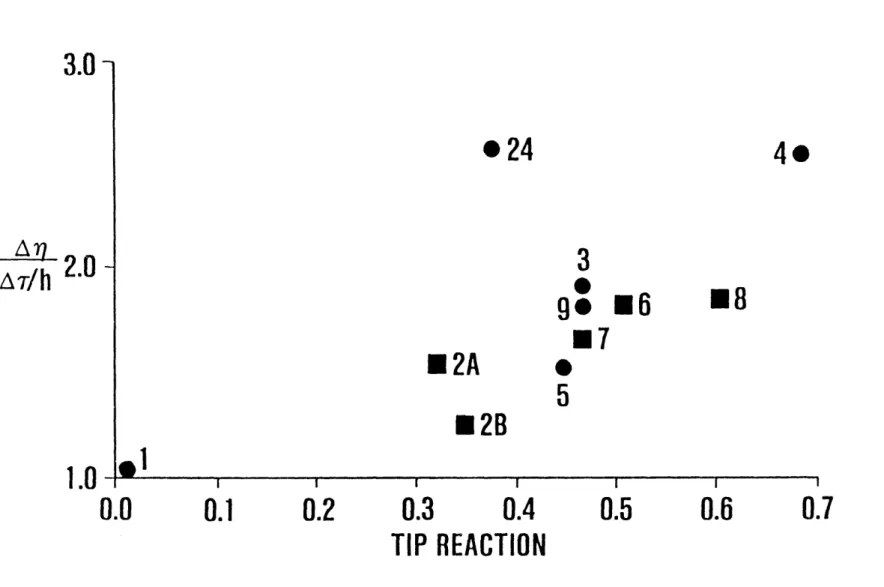
are expected to show maximum values at some intermediate degree of reaction, For the same reasons, the difference between the relative gap 8/H and relative leakage rate, X, will also peak at that intermediate R.These trends are shown in Figs. 6 and 7. Here the leakage )L was held at 0.1 and the degree of reaction R was varied over the range 0-1, while the flow coefficient O was given values from 0.3 to 0.7. Zero exit swirl was assumed, and so different O values imply different turbine angles P3, while varying R amounts to varying the stator blade angle
a2. The expected peak in loss factor is seen to occur for R 0.8, which is higher than the practical range for turbines (0 - 0.6 or so). Hence, in practice, the expected trend would be for losses to increase with degree of reaction. This trend is clearly exhibited in Waterman's data
compilation(3), as indicated in Fig. 8 (taken fom Ref. 3). More detailed data analysis will be shown in Secs. 6.2 and 9.2. The minimum of 8/H at R = 0.8 shown in Fig. 7 confirms that redistribution effects are indeed
strongest then, since the smallest gaps is required to pass a given leakage.
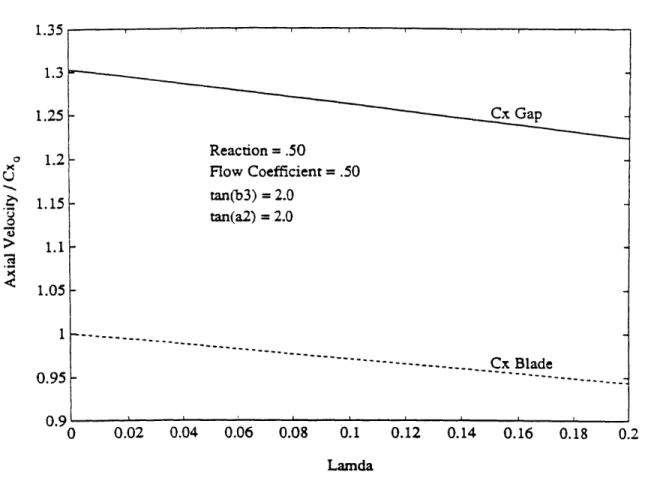
So far parametric results ("rubber engine") have been discussed. For a given turbine (given X2, 03) some trends are shown in Figs. 9 and 10. Fig. 9 shows the two axial velocity levels at the disk as the gap only is varied (as reflected in the leakage rate). While both velocities vary only slightly with gap, it must be remembered that for the bladed
region, it is the difference I -x, that controls the losses, and this difference does have a substantial variation. On the other hand, the "jet" velocity changes are not particularly significant, as one would expect, since they mostly respond to the fixed AP across the turbine. O f course the word "jet" must be used with caution, since only the
x-component of the velocity is shown.
In Fig. 10 all geometrical parameters, including gap size, are fixed and the flow coefficient is varied. This allows non-zero exit swirl to occur (ranging from C o/CX, = 0.73 at 0 = 0.27 to CO/c, - 0.47. at
$ = 0.4, with zero exit swirl at $ = 1/3). As the flow varies, the degree of reaction remains approximately fixed (close to the design value of
0.5), but turbine loading To increases with
4,
as shown in the lower scale. As the results show, the tip leakage fraction remains at about 1.5 times the relative gap throughout. On the other hand, the loss factorp
increases strongly with flow, and weakly with decreasing gap.6.2 Comparison to Turbine Data
We can now compare the calculated losses to those
reported in the experimental literature. We rely for this on the compilation of Ref. 3, which gives data for ten cases (nine different turbines) over a wide range of parameters. Ref. 3 reports for each case the tip values of the work co-efficient To (two definitions), degree of reactor R, flow coefficient 0, and individual blade loading (lift
coefficient cL, based in inlet relative velocity and blade area, and Zweifel coefficient (tangential force coefficient based on tangential area and exit dynamic head). Also reported are the relative gap and, in some instances, other geometrical parameters. As noted in the
Introduction, Ref. 3 also shows the results of several existing loss correlations or theories when applied to these cases, plus the actual measured loss factor
P.
One potential difficulty in application is that only "jg parameters are given, whereas from the nature of our theory we suspect that mean parameters might be more appropriate.
Starting from Vo (with the definition which agrees with that in our Appendix B), 0 and R, the equations in Appendix B allow
calculation of the blade angles a2, P3. The fractional leakage, X, is
determined from the relative gap 8/H using Eq. 51. This involves the shear strength q, which itself depends somewhat on X, so some iteration must be used. The remainder of the calculations is straightforward. Table 2 summarizes the results
Scanning Table 2 we first notice a large disagreenment for Case I (Kofskey turbine). This is an impulse rocket turbopump stage with extremely large reported tip loading (W = 7.0). As the table shows, this leads to very large exit swirl (c/cx.= - 3.2). No reasonable modification of the theory could be found to resolve the disagreement of the
f
calculated and that reported, which, as expected for a low-reaction stage, is low (P = 1.02). A calculation was made, as shown in the second from-last-row of table 2, with a load To reduced to 2.0, which leads to near-axial exit flow, and this does predictP
= 0.97, close to the measured value. This might indicate a large radial load gradient for this turbine, but this has not been investigated futher.Excluding Case 1, the mean squared error in the predicted 0 is
E2
~
(DATA - OCALC2 = 0.1434N
This compares favorably with the results of applying the correlations of Kofskey, Ainley, Soderberg and Roelke (See Table 1). The mean error
is C = DATA - CALC = 0-1434
NN
which idicates a general under-prediction of the losses. The standard deviation is
Y=e
-T7 0.337
7. Numerical Verification
The linearized solution has yielded important results, some of which defy our expectations. It is therefore important at this point to investigate the extent to which these results may have been
compromised by the linearization. To this end, we need to solve by a numerical technique the complete non-liner actuator disk problem (Eqs. 28, 29). Inverse coordinates are still a convenient formulation, especially in that they fix the location of the shear layer along a coordinate line
(T = PTIP, X > 0), thus avoiding the smearing inherent in any discontinuity-capturing approach that could be used in direct (x,z) coordinates. Simple finite differences on a rectangular grid can also be used effectively with such a formulation, since the main surfaces (disk, walls, shear layer) are all aligned with the coordinate lines (x,'P). The only disadvantage is the more complex form of the Laplacian
in these coordinates (see Eq. 32).
The method used is a form of over-relaxation, which can be constructed starting from a minimum principle for the problem (See Ref. 12 for details). Care is taken to include the 8 functon on the right-hand side of Eq. (28) in a consistent manner. Integrating Eq. (28) across the shear layer, and, as before, using superscripts (+) and (-) for the gap and bladed sides, respectively, one obtains at each x
(1+z2)1 -
2Q
(z)2 (zq,)2
76)where Q is calculated from disk vewlocities according to Eq. (27). In discretizing the connecting condition (76), one-sided differences are used for zq and z, to avoid numerical "mixing" of the two streams. Most of the calculations were done on a 16 x 32 grid. As a check, one case was computed on a 24 x 48 grid, and the discrepancies (Table 3) were found to be below 10-3 in relative terms.
A series of numerical results showing the two velocity components at the disk, with the linearized theory results
superimposed, are given in Figs 11 through 26. For degrees of reaction below 0.4 or above 0.90 the agreement is excellent. As expected, the worst linerarization errors occur in the vicinity of R ~ 0.8 , but even then the results of the linear theory are found to be fairly accurate. Most importantly, the prediction that the axial velocity at the disk is piecewise constant is clearly borne out by the nonlinear results. The only noticeable deviation from throughflow uniformity in the bladed region occurs very near the blade tip (on the scale of the gap size), and its integrated effect is in any case minimal.
8.1 Introduction
One of the basic approximations made in the theoretical
treatment so far is that of zero work done by any fluid crossing the gap area. If we include under that description any streamline which passes over one blade tip, this is clearly not an accurate assumption. Fig. 27,
for example, shows that, prior to crossing over, a streamtube is partially deflected by the blade, and hence does some push work on it. The
magnitude of this work could be quantified if the flow angle for the leakage fluid leaving the passages were known, which prompts us to a more detailed examination of the flow field around the blade-tip gap region.
The blade-tip region has been theoretically treated using a variety of approaches. The simple model of Rains(4), which is most appropriate for thin, lightly loaded blades, uses ideal, pressure-driven flow concepts to derive the speed and direction of the gap "jet". Even for the case of the thicker turbine blading, ideal flow is a fairly good approximation. For example, Rains(4) gave a criterion for viscous forces to be negligible, in the form
A GAP 2 x THICKNE-5) x R (CHORD, REL. INLET, VELOCITY) > 125
THICKNESSY CHORD
(78)
For the experimental turbine being tested as part of our research on Alford forces, this parameter is approximately 1000, and this situation is quite common. On the other hand, the effects of chordwise pressure gradients on thick-blade tip flows, as well as that of relative wall motion are still potentially significant, and have not been treated so far.
The gap jet is known to interact strongly with the passage flow and to roll itself up into a concentrated vortex-like structure. Rains
himself derived (4) a semi-empirical expression for the trajectory of that vortex. Lakshminarayana (6,7) also used empirical information on the tip vortex location and strength to predict details of the blade pressure distribution, In fact, the strength of the vortex was explicitly related to a "partial blade-tip loading parameter", K, varying from 0 to 1,
and inferred from extrapolation of surface pressure measurements near the tip to the end wall. Since there are very sharp pressure
gradients in the pressure side of the blade, near the gap, this procedure is fraught with difficulties. More recently, G.T. Chen et al (13) have used vorticity dynamics to simulate the roll-up process, and have been able to predict accurately the trajectory of the vortex.
In what follows, we will introduce an alternative viewpoint which leads to simple, but accurate expressions for the location and size of the leakage vortex. This can then be used in calculating the flow leaving angle of, and hence the work done by the leakage flow.
8.2 Collision of the Leakage Jet and the Passage Flow
Fig. 28 shows schematically the essential features of the leakage flow. The fluid approaches a blade (here represented as a flat plate) with a relative velocity w2, which evolves into the passage flow velocity WPAss
at locations not very near the tip gap. Under the action of the pressure differential across the blade, a jet of leakage flow at velocity Wjet escapes under the blade. This jet penetrates a certain distance into the passage, but is eventually stopped by the main flow, which separates the jet from the wall, turns it backwards, and leads to the formation of a rolled-up structure containing both, leakage and passage fluid. This "collision" of the two streams is again shown in Fig. 29 in plan form, and Fig. 30
shows a schematic of the flow structure seen in a cut such as a-a in Fig. 29, with leakage fluid shown dashed.
Consider the situation at points along the jet separation line, such as P in Figs. 29,30. Ignoring frictional effects, the two streams which meet there (jet and passage flows) can both be traced back along different paths, to the inlet flow, and hence have equal total pressures and temperatures. Since they also have equal static pressures along their contact line, (and generally similar static pressures throughout
the section a-a is perpendicular to OP, we can think of pont P (Fig. 30) as the common stagnation point of the two "colliding" flows, approaching each other with equal velocities, which are each the component of Wjet
and WPAss perpendicular to line OP. It follows that line OP must bisect the angle made by Wiet and Wrass This gives a first and important piece of information about the location of the rolled up structure, but, since this structure has a finite and increasing transverse dimension, it does not yet locate its center.
To continue our discussion, notice that the transverse momentum balance of a fluid element near point P requires that both transverse colliding flows must bring equal (and opposite) momentum fluxes to the rolled-up structure. Since the two velocities are equal, we find that equal mass flows must be entering the rolled-up structure from both fluids. In other words, the clear and dashed areas in Fig. 30 must occupy equal fractions of the total "vortex" cross section. Let 8 JET be the jet thickness, and Wi, w1 the common components along and across OP of
the colliding streams. The rate of increase of the cross-section A1 of the
rolled structure along OP is then given by
W dAL= 2 w1 JET
ds (78)
0
=tan.1 WIor, callling WII, i.e., the angle made by the separation line OP and the blade itself,
dA_ = 2 8JET tan
0
ds (79)
where s is measured along the vortex trajectory.
The precise shape of the rolled-up structure is more difficult to establish, but it seems reasonable to model it as (half) cylindrical ideal vortex in a cross-flow. Following Batchelor(14) such a vortex is describable by the stream function (Fig. 31)
where R is the radius of the dividing streamline, J1 (x) is the Bessel's
function of the 1st order (with a zero at x = 3.83) and (r, (1) are polar coordinates. The vorticity in this flow is distributed inside the semi-circle of radius R in proportion to T:
CO
3.8 3
\
R
(81)
and is zero outside. Integration of (O gives an overall circulation
['= 6.83 w1 R (82)
whereas integration of r sin 0 (0 gives a center of vorticity height of
ze = 0.460 R (83)
We thus make A1 =7rR2, and measuring distance along the blade
(xBL = S cos 0), we can integrate Eq. (79) to obtain
R=
4TtanO
6JET XBL
7
L cos0 (84a)
The trajectory of the vortex center then follows (Fig. 32) as
yc= XBL tanO- R
cos 0 (84b)
To complete the analysis, the angle 0 must now be determined. From our discussion of the separation line OP, this angle was shown to be half of the angle P between the blade and the jet flow:
0= P/2 (85)
This angle P follows from the simple local analysis first proposed by Rains(4), which applies to thin blades when viscous effects can be neglected, In Fig. 33, wp and Ws are the flow velocities on the pressure
and suction sides of the blade, respectively. Application of Bernoulli's equation relates these velocities to the corresponding pressures:
wp= w2 2 -2 P2
P (85)
(86) where P2, w2 corresponds to inlet conditions. On the other hand, the
leakage jet emerges form the gap with a velocity component perpendicular to the blade of
WG 2
2
p (87)
and its components parallel to the blade is simply wp, since no
momentum is added or lost in that direction during passage throught the gap. It can be verified that the net magnitude wJET of the jet velocity is then equal to ws, as indicated previously. We then obtain (Fig. 33)
tan
$
(88)where c = 2((P-P2))/p w2 in each case. Note that (cp)p -(cp)s is the local
lift coefficient cj, referred to the relative turbine inlet velocity. Using the half-angle trigonometric formulae,
tan 0 =
-14
1 _-(C,) + f 1 -(C4 (89)Notice that, as shown in Fig. 33, the vorticity vector
corresponding to the shear between the jet and the adjacent passage flow is inclined at 0 = P/2 w.r.t. the blade, i.e. it is parallel to the outer edge OP of the rolled-up structure, This is also the direction of the mean flow between the two sides of the shear layer, which means that the shear vorticity is not convected at all towards the line OP. The only reason the vorticity F rolled up into the structure increases with downstream distance is that the growth of R gradually overlaps more and more of the shear vorticity. In this sense, the commonly invoked view of the rolled-up vortex growing by the connection of shed vortices must be used with caution.
Eqs. (84a), (84b) and (89) can now be used to calculate the vortex geometry if the suction and pressure side Cp distributions are know from experiments or calculations. A simple approximation can be obtained using the theory of lightly loaded thin wing profiles. In this approximation, (wp+ wY2 w2, which when used in Eq. (85, (86)
reduces both (Cp)p and (Cp)s to functions of c = (Cpp - (Cp)s alone. Using this in Eq. (79) gives finally
(C , (<4)
S= cos
1,4+cL
(L4CL
4+cj
(CL>4)(90)
Notice the relative insensitively of 0 to CL, particularly about he common value c' = 4, when 0 reaches a maximum of 450*.
8.3 Comparison to Vorticity Dynamics Model and to Data
Ref. (13) has recently provided a means of correlating a varitey of rolled-up vortrex data using a similarity analysis. Transverse
distances are normalized by gap width 8, and axial distance, or time-of-flight are characterized by a parameter
x
X P (91)
where x and Cx are axial distance and velocity and AP = Pp- Ps. The data from many experiments (mainly from compressor cascades) correlate well with t*. In addition, a calculational method was developed in Ref.
13 to track a series of shed tip vortices from an impulsively started plate, which represents the situation seen from a convective frame as the flow passes over a blade. The calculated results were shown to also correlate well with t* and and with the data.
We use the correspondence
-X-= cos $2 , X =Cos $M
W2 XBL (92)
where
$2
and Pm represent the relative flow angles at the rotor inlet and on average in the rotor, respectively, to deriveXBL _ W COS$2 t*
8JET wG COS pm (93)
where j= JET/6 is the gap discharge coefficient. Note also that W2 =
1/
WG .
p.=0.785
C
=
1.35
= 1.1
COS P
to relate t* to our XBL, and then calculate the vortex trajectory using Eqs. (84a), (84b), (89) and (90). The results are compared in Fig. 34 to those reported in Ref. (13). The agreement with the data is satisfactory. Additional verification against the theory of Ref. (13) can be provided by comparing the predictions of both theories regarding the "center of vorticity" location in a cross-plant similar to that shown in Fig. 30. in order to be consistent with the calculations of Ref. (13), we have included here both, the rolled-up vorticity IF (Eq. 83), and a vorticity 2w1 per unit length (perpendicular to o0) of the not-yet-rolled shear
layer.
In calculating the distance ze between the center of vorticity and the wall, we took this latter contribution to be at a distance 6JET, and that of the rolled-up vortex to be at 5
JET + 0.46R (Eq. 82). The results are shown in Fig. 35, which again shows good agreement between our method and that of Ref. 13.
9. Blade-Tip Losses Including Partial Tip Loading
9.1. Modications of the Actuator-Disk Model
We now abandon the assumption of zero work done by the
leakage fluid. This is somewhat less drastic a step then it might seem to be. Conceptually, we will now claim that the fluid which crosses the gap between the casing and a turbine blade is only partially underturned when compared to passage fluid. The fractional work done per unit mass of this leakage fluid will turn out to be about 50%, typically. On the other hand, this fluid "collides" with passage fluid and coalesces with it, leaving the rotor mainly in the form of a rolled-up vortex which
includes 50% each, gap and passage fluid. Thus, an equivalent amount of passage fluid ends up being underturned as well. These two effects, partial under-turning of gap fluid, and partial under-turning of vortex-entrained passage fluid, tend to add up to the same net result as in the more idealized model considered so far.
There are three specific modifications to be made to the theory in order to incorporate these effects:
(a) Re-defining the"leakage flow fraction", X, to include all under-turned fluid. Of this, only the fraction X/2 is gap flow, and this is what must be related to the physical gap, 8 (Eqs. 51 or 52).
(b) Allowing a non-zero total enthalpy drop for the gap flow, and relating it to the angle 0 by which the flow fraction X under-turns. This angle is supplied by a form of the theory of Sec. 8.
(c) Recognizing that the fluid comprising X has not undergone an isentropic work-producing process, since formation of the rolled-up vortex is intrinsically lossy.
The under-turning angle 0 should be calculated as an average which includes the rolled-up flow, assumed to have its momentum directed along the centerline of the rolled-up vortex, and also the portion of the gap jet which is not yet rolled up at exit (similar to the calculation described in Sec. 8.3 for the center of vorticity). In the interest of simplicity, we will take 0 to be as given by Eq. (85), i.e., the angle between the blade and the outer edge of the vortex (Figs. 32, 33). This will to some extent cancel the modifications due to, on one hand, the angle between this outer edge and the vortex centerline, and, on the other hand, the contribution of the un-rolled jet, which is more
strongly under-turned.
Let Pm be the average angle of the rotor blades to the axial direction which can be calculated (Fig. 4) as
PM- 3 - ( 2)DES.
2 (94)
with tan (P2)DES = tan X2 - = tan X2 - tan P3 (95)
ODES
The passage flow relative velocity is then (on average)
WPAss =
Cos hM which has components wgl and wj. parallel and perpendicular to the
vortex
Wi x ": Cos
0
; w-CX sine
COS m COsjm (96)
The gap flow, for its part, has components w11 and -wI in the
same directions. The flow fraction A is all assumed to leave the passage with velocity WI along line OP, and so its relative Y - component of velocity is wi1sin ($m -0). In the absolute frame, then,
+ _ Cos 0 sin ($M - 0)
cy3 = U - c s
Cos PM (98)
where we use the (+) superscript as before to denote the "gap fluid", which now, more precisely, means all of the under-turned fluid. Of
course, the rest of the fluid has a Cy3 = cy3 still given by Eq. (57).
Also, the disk axial velocities Ct , CjX are still as given by Eqs. (46), although
Q
will now be different. Notice that Eq. (98) replaces the previously used non-turning assumption (cyi = cx tana
2)Application of the Euler equation to both fluids gives the work done per unit mass by each stream:
W+= U (ct tan a2 - cy)
W-= U (cx tan
a
2 - cy3) (99a,b)and, since ideality is assumed in the bladed region, pW- is the same asd the turbine total pressure drop in that region, i.e.
W- = BI - B- = B1I - BI - (cy3)2
2 (100)
In the "gap region", however, W+ is less than the isentropic work B1 - B+ by an amount TAS equal the energy dissipation incurred
in the mixing of the gap and passage streams. Per unit mass, this dissipation equals the kinetic energy associated with the "destroyed" component W1 of Eq. (96):
TAS=
(et
sin 0
2 Cos PM (101)
W
B
- B - (cy3P - (c+) sinL1~o
2
$
CO /N (102)Subtracting Eqs. (100) and (102), and remembering that
Q
= B7 - B, we obtainQ
=
W-
- W+ -(c)
sin 02 -
(cy+)2 +-(CY32
\COS m/22 (103)
We can now use Eqs. (88) and (57) for the Cy's, and then Eq. (46) for the cX's and, upon substitution into (102), we obtain the new
equation for q. Rearranging this takes the form
(1-k2G
- X2tan 2P3]
(SY+ 2
2 +tan a
2+
(1-
X) G +
Xtan2pm1
--(tan 2 3 -G)= 0 (104)
where G
(cose
sin(m
-
e)
+
sinem
\
cos M
/
\cos
mI(105)
which replaces Eq. (47).
Once q is calculated, the total turbine work per unit mass is
XW+ + (1 - ) W-. Normalizing,
V
=V0 -~~
X0$(tan P3 - g) 1+2
q(16
q)(106)where g
=(cos
sin ($m -0)COS M (107)
The calculation of the total pressure drop is identical to that
explained in Eqs. (58) - (61), except that, as mentioned cY3 is now given
by Eq. (98) rather than Eq. (56). In particular,the static pressure drop still follows from Eqs. (61 and (23), since only ideal flow
through the bladed region is involved. Following calculation of
Pto - PtMIX., the efficiency and the loss parameter can be found as before
In order to compare the modified theory of Sec. 9.1 to the same turbine data as before (Sec. 6.2), additional data regarding individual blade loading are needed to calculate the under-turning angle 0. This information is contained in the Zweifel coefficient ZW, which is also reported by Ref. 3 in each case, This is related to the blade lift as shown in Appendix B (Eq. B 11). The angle 8 then follows from Eq. 90, where the overall lift coefficient CL is used as a representative value of the local c'L
The results for the same set of data as was used in Sec. 6.2 are summarized in Table 4, where the entries are the same as in Table 2, except for ZW and the last column, labelled K, which is the ratio of work done per unit mass by the underturned flow to that done by the blade-guided flow:
K
- W+W- (108)
Once again, Case I can only be brought into agreement with the data if the load factor is reduced to about the design value (i.e., for zero exit swirl). Case No. 4, with very high reaction, is also substantially under-predicted, which may point ot an insufficient predicted underturning 0 for these conditions. The rest of the cases are well predicted. Excluding Case 1, as before, the mean squared error is
2 0.1162
and the mean error is = -0.1408
which imply a standard deviation a = 0.3105
These statistics are slightly better than those found for the zero tip loading theory (Sec. 6.2), and, although they compare favorably with those for the standard methods, they also still show some systematic
under-prediction and moderate scatter. It is of interest that most of the error and scatter (other than that due to point 1) is caused by the
single high-reaction data point (Case 4). If that entry were also removed, we would have E2 = 0.0363, = - 0.0498 and G = 0.184.