M
by
Rory Kirchner
B.S., Rochester Institute of Technology (1999)
Submitted to the Department of Health Sciences and Technology
in partial fulfillment of the requirements for the degree of
Doctor of Philosophy in Health Sciences and Technology
at the
MASSACHUSETTS INSTITUTE OF TECHNOLOGY
September 2015
D Massachusetts Institute of Technology 2015. All rights reserved.
Signature redacted
Department of Health S ences and Technology
Septem
2015
Author. .
Certified by...
Acrented
by
Signature
Professor of E
redacted
Martha Constantine-Paton
rain and Cognitive Science
Thesis Supervisor
Signature redacted
. . . .
. . . .
Emery N. Brown
Director, Harvard-
Program in Health Sciences and Technology
Professor of Computational Neuroscience and Health Sciences and
Technology
ASSA HUSETS INS ITUTE
RSEP
24 2015
LIBRARIES
Automated, highly scalable RNA-seq analysis
by
Rory Kirchner
Submitted to the Department of Health Sciences and Technology on September 1, 2015, in partial fulfillment of the
requirements for the degree of
Doctor of Philosophy in Health Sciences and Technology
Abstract
RNA-sequencing is a sensitive method for inferring gene expression and provides ad-ditional information regarding splice variants, polymorphisms and novel genes and isoforms. Using this extra information greatly increases the complexity of an analysis and prevents novice investigators from analyzing their own data. The first chapter of this work introduces a solution to this issue. It describes a community-curated, scal-able RNA-seq analysis framework for performing differential transcriptome expres-sion, transcriptome assembly, variant and RNA-editing calling. It handles the entire stack of an analysis, from downloading and installing hundreds of tools, libraries and genomes to running an analysis that is able to be scaled to handle thousands of samples simultaneously. It can be run on a local machine, any high performance cluster or on the cloud and new tools can be plugged in at will. The second chapter of this work uses this software to examine transcriptome changes in the cortex of a mouse model of tuberous sclerosis with a neuron-specific knockout of Tscl. We show that upregulation of the serotonin receptor Htr2c causes aberrant calcium spiking in the Tscl knockout mouse, and implicate it as a novel therapeutic target for tuberous sclerosis. The third chapter of this work investigates transcriptome regulation in the superior colliculus with prolonged eye closure. We show that while the colliculus undergoes long term anatomical changes with light deprivation, the gene expression in the colliculus is unchanged, barring a module of genes involved in energy produc-tion. We use the gene expression data to resolve a long-standing debate regarding the expression of dopamine receptors in the superior colliculus and found a striking segregation of the Drdl and Drd2 dopamine receptors into distinct functional zones. Thesis Supervisor: Martha Constantine-Paton
Acknowledgments
Thank you to the members of the Constantine-Paton Lab, Robert and Ellen Kirchner, my parents, Dr. Melcher for her unwavering support and to the Imaginary Bridges Group.
1 Automated RNA-seq analysis
11
1.1 Background . . . .. . . . . 12
1.1.1 RNA-seq ... ... 12
1.1.2 RNA-seq processing challenges ... 13
1.1.3 RNA-seq analysis pipelines . . . . 15
1.1.4 Scalability . . . . 17
1.1.5 Reproducibility . . . . 23
1.1.6 Configuration . . . . 24
1.1.7 Q uantifiable . . . . 25
1.1.8 RNA-seq implementation . . . . 31
1.1.9 Variant calling and RNA editing . . . . 45
1.2 D iscussion . . . . 47
1.3 Future development . . . . 48
2 Transcriptome defects in a mouse model of tuberous sclerosis
50
2.1 Background . . . . 502.1.1 Tuberous sclerosis . . . . 50
2.1.2 Tuberous sclerosis is a tractible autism model . . . . 59
2.1.3 The second order effects of mTor activation are important 2.2 Methods . . . .
2.2.1 Cortex collection . . . .
2.2.2 Library preparation and sequencing . . . .
2.2.3 Informatics analysis . . . .
2.2.4 Calcium Imaging . . . .
2.3 R esults . . . .
2.3.1 Differential expression . . . .
2.3.2 Pathway analysis . . . .
2.3.3 Isoform differential expression . . . . 2.3.4 Disease association . . . .
2.3.5 RNA editing . . . .
2.3.6 Syn1-Tsc1-/- mice have aberrant calcium signaling.
2.3.7 Htr2c blocker halts aberrant calcium signaling . . . 2.4 Discussion . . . . . . . . 63 . . . . 63 . . . . 64 . . . . 65 . . . . 67 . . . . 68 . . . . 68 . . . . 75 . . . . 75 . . . . 76 . . . . 80 . . . . 81 . . . . 83 . . . . 83
3 Transcriptome independent retained plasticity of the
corticocollic-ular projection of the mouse
87
3.1 Background .... . . ... ... . . . . . . 873.1.1 Superior colliculus . . . . 87
3.1.2 Retinotopographic map formation in the colliculus . . . . 91
3.2 M ethods . . . 100
3.2.1 Eye closure manipulation and colliculus dissection . . . 100
3.2.2 Total RNA isolation and quality control . . . 101
3.2.3 cDNA Library creation and sequencing . . . 104
3.2.4 Informatics analysis . . . 105
6
3.2.6 Corticollicular projection mapping and quantitation . . . 106
3.3 R esults . . . 107
3.3.1 Corticocollicular projection remodelling . . . 107
3.3.2 Sequencing quality control . . . 108
3.3.3 Differential gene expression . . . 108
3.3.4 Possible X-linked cofactors in LHON . . . 113
3.3.5 Differential exon expression . . . 114
3.3.6 Dopamine receptor expression in the superior colliculus . . . . 114
3.4 Discussion . . . 116
List of Figures
1-1 collectl benchmarks of hourly memory, disk and CPU usage during a
RNA-seq analysis. . . . . 19
1-2 Schematic of parallelization abstraction provided by ipython-cluster-h elp er. . . . . 20
1-3 The Poisson distribution is overdispersed for RNA-seq count data. . . 30
1-4 RNA-seq differential expression concordance calculation from two sim-ulated experiments. . . . . 32
1-5 Schematic of RNA-seq analysis. . . . . 34
1-6 Tuning adapter trimming with cutadapt . . . . 36
1-7 Gene level quantification can introduce errors. . . . . 39
1-8 RNA-seq improves the rat transcriptome annotation. . . . . 44
2-1 CNS manifestations of tuberous sclerosis. . . . . 51
2-2 The mTor pathway is affected in many disorders with autism as a phenotype. . . . . 54
2-3 The laminar structure of cortex in Syn1-Tscl-/- mice is undisturbed. 58 2-4 MA-plot of gene expression in the cortex of wild type vs. Synl-Tscl--litterm ates. . . . . 69
2-6 Blocking the Htr2c receptor halts aberrant calcium spiking in
Syn1-Tscl-/- neurons. . . . . 84
3-1 Cell types of the superior colliculus . . . . 90
3-2 Eye opening refines the corticollicular projection. . . . . 99
3-3 Schematic of superior colliculus dissection. . . . 102
3-4 Effect of eye closure state on corticocollicular arbor development. . . 109
3-5 Trimmed mean of M-values (TMM) normalization effectively normal-izes gene expression. . . . 110
3-6 Clustering of gene expression in the rat colliculus. . . . 111
3-7 MA-plot (mean expression vs log2 fold change) between eyes open and closed rats. . . . 112
3-8 MA-plot of differential exon analysis. . . . 115
3-9 Dopamine receptor subtypes are segregated into distinct layers of the superior colliculus. . . . 117
List of Tables
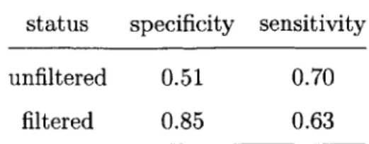
1.1 Cleaning the raw Cufflinks reference-guided transcriptome assembly improves the false positive rate. . . . . 43 2.1 Differentially expressed genes in Synl-Tscl-/~ mice. . . . . 75
2.2 KEGG pathway analysis of differentially regulated genes . . . . 76 2.3 Gene Ontology (GO) term analysis of differentially regulated genes. 77
2.4 mTor signaling is differentially regulated in the Syn1-Tsc-/- mouse. 78 2.5 Autism, intellectual disability and epilepsy genes differentially
regu-lated in the Syn1-TscEl-/- mouse . . . . 79 2.6 RNA editing events found in Synl-Tsc-/- and WT mice. . . . . 80
3.1 Power estimation of the eyes open vs. eyes closed experiment at a range of fold changes . . . 106
Automated RNA-seq
analysis
RNA-sequencing (RNA-seq) has largely supplanted array-based methods for infer-ring differential expression at the gene, isoform and event level as RNA-seq is more sensitive and produces more information than array-based methods at a similar cost. However processing RNA-seq data and making use of the extra information that comes from having sequence data is complex and experiment dependent. Further-more what is considered best practice is constantly changing which presents a re-searcher with many choices of how to perform each step of an analysis. Analyzing a large RNA-seq dataset requires access to a high performance computing cluster, either locally or via the cloud. Even a moderately sized RNA-seq experiment can be hundreds of gigabytes in size and if care is not taken with the choices of tools, they may not operate properly on data of this scale. This chapter describes the RNA-seq module implemented for this thesis as part of the bcbio-nextgen project, a
community-developed, highly scalable and easily installable set of analyses of whole genome and exome variant calling and RNA-seq data. This software is in use in academic research labs, core facilities and pharmaceutical companies all over the world, is downloaded thousands of times every month and has processed thousands of RNA-seq samples for hundreds of researchers all over the world[37].
1.1
Background
1.1.1
RNA-seq
RNA-sequencing has largely supplanted array-based methods for quantifying gene-expression. Array based methods estimate gene expression by attaching small an-tisense probe sequences designed to bind a subset of the transcriptome to a slide. Query sequences are fragmented, labelled with a fluoroescent dye and hybridized to the array. The luminance at each spot on the array is measured and used as a proxy for the expression of the gene the probe is designed to target, assuming a one to one relationship between the probe and the target gene[125]. This approach has some limitations. The first limitation is that only known genes can be assayed, because the probe sequences must be designed from known transcripts. The second is that because the quantitation is based on luminance, the dynamic range of the measurements is constrained to just a few orders of magnitude, as at one end the luminance falls below the level of noise and at the other end the camera is saturated. The third limitation is that, for the most part, only gene expression can be assayed using this approach. RNA-seq removes some of the limitations of array analysis. RNA-seq assays gene expression via the sequencing of small fragments of cDNA up to hundreds of bases in size called reads, aligning the reads to the genome of interest
and estimating the overall expression by counting the number of reads aligning to each gene[186]. Since alignment to the genome is not dependent on the state of the transcriptome annotation it is theoretically possible to infer new genes and isoforms strictly from alignments of the reads to the genome. As new genome builds are
cre-ated and new annotations layered on top of them old data can be further mined for new information by realigning to the new genome build and reanalyzing the gene expression using the updated annotation. Since quantitation of gene expression is based on counting the number of reads aligning to a gene, the dynamic range is limited by only how many reads are sequenced, lending a much higher sensitivity at the low and high end of the expression spectrum over array based methods. Finally,
by examining differences in the sequence of the reads aligning to the genome, it is
possible to call variants and RNA-editing events from RNA-seq data. The increased power does not come for free, however. Making use of this extra information makes the analysis of RNA-seq data much more complex and places more computational demands on researchers.
1.1.2
RNA-seq processing challenges
There are several major challenges when handling RNA-seq data. RNA-seq data is very heterogeneous, there are many choices at each stage of performing a RNA-seq experiment, starting at choices of how to extract and purify and fragment the RNA, the type of library preparation performed and the type of sequencing to be performed. Sequencing can be from one end of the RNA fragment (single) or both ends (paired), with a range of lengths of reads and insert sizes of the RNA fragment between the pairs. In addition, RNA-seq data can be from one of several strand-specific protocols where information regarding the strand a gene is on is preserved during sequencing,
which affects the downstream analysis. Finally there are several types of sequencers and each type of sequencer produces reads with varying characteristics and error profiles, all of which need to be taken into account during an analysis. As a result of these complexities it is difficult to have a simple one-size fits all analysis pipeline that can handle a wide variety of experiments. Thus, RNA-seq analysis in published papers tends to be experiment-specific and difficult to reproduce. We have solved this problem by implementing a flexible analysis pipeline that can handle many different types of RNA-seq experiments.
In addition to being very heterogeneous, RNA-seq data can be very large and com-putationally complex which adds to the difficulty in analysis. A single lane of data can be tens of gigabytes in size and a large scale RNA-seq experiment can encompass hundreds of lanes or more. Memory and CPU requirements for most programs mean most analyses will not be able to be run on common lab computers and will have to be run on either large-scale shared cluster compute environments or cloud-based compute environments. These compute environments themselves are very hetero-geneous, with differing storage backends, shared and non-shared filesystems, ways to distribute jobs to a cluster via cluster schedulers, heterogeneous CPU and mem-ory availability on nodes, operating systems and other complexities relating to the hardware the analysis is run on. Not only must an analysis pipline be able to run in varied compute environments, it has to be able to process data across a wide range of scales from single samples to thousands of samples. We have solved these problems in bcbio-nextgen by abstracting the compute environment away from the analysis with a small library called ipython-cluster-helper. The ipython-cluster-helper
library has been used in several other projects to provide scaling across all available high performance computing schedulers[129][128).
Another area of challenge is the large choice of tools for performing each step
in an analysis. There are a myriad of programs available to perform every step in an analysis, from quality control of the raw reads, aligning[54], assembly[58][163] and quantification[46] of transcripts, differential expression[144] and final quality control [45] [62] of the results. Often times it is not clear what the tradeoffs are when choosing one tool over another, and some tools may not function properly with large datasets or with data from a particular sequencer or type of experiment. Each tool for each step in an analysis is configurable and determining how to properly configure each tool for a specific analysis is complex, time consuming and prone to error. For some tools it can be difficult to even install the tool, especially on shared compute environments where necessary libraries may not be installed or administrator priv-ileges might be needed to install some programs. In addition each tool may need special data files in a wide variety of formats to work properly and producing these data files from the known genome and transcriptome can be a challenging task.
All of these challenges make it extremely difficult for a researcher without
pro-gramming experience and without a deep knowledge of UNIX to even get started analyzing their own data. In addition, all of these challenges make performing anal-yses in a reproducible way very difficult; at the end of an experiment it is often impossible to trace what was run on each sample much less reproduce the analysis using the same tools with the same data.
1.1.3
RNA-seq analysis pipelines
As of July, 2015 there are 200,000 Google results for 'RNA-seq analysis pipeline' but very few of those are under active development and have kept up with the state of the art and none of them install everything you need to run a RNA-seq analysis. A poll on the RNA-seq blog in July 13th, 2013 asked 'What is the greatest immediate
need facing the RNA-seq community?' with ~ 70 % of the responses being either a need for a standardized data analysis pipeline or more skilled bioinformatics experts to process the data. The rate of generation of sequencing data is far outpacing the generation of skilled bioinformaticians so it will be important to have an accurate, flexible, validated RNA-seq pipeline that can be run by a naive researcher in order to keep up with the rapidly increasing amount of generated sequencing data. The need for this is reflected in industry; in December, 2014 Bina, a company that has implemented a variant calling and simple RNA-seq analysis pipeline was bought by Roche and a myriad of startups have sprung up, promising to handle the analysis of second generation sequencing data either on local appliances or the cloud. It is important for a free, community developed, open source alternative to these industry pipelines to exist because many academic labs will not have funding to run on these commercial appliances.
It is important to specify what characteristics a standardized, scalable and re-producible RNA-seq analysis pipeline should have. The first is that it should be configurable at a high level of abstraction. A proper pipeline should translate a small set of high level options to the appropriate low-level settings for each tool in a pipeline. These exposed options should be a minimal set to accurately run an analysis, with as many of the low-level options as possible derived from the data. A researcher should not have to be familiar with the intricacies of each tool in order to run an analysis. The second characteristic of a standardized RNA-seq analysis pipeline is it should be reproducible. A full accounting of the versions of all third party tools that were used along with all of the commands that were run should be provided at the end of an analysis so the analysis can be reproduced. Ideally a Docker container with all of the relevant software installed would be distributed along with the raw data so any researcher could reproduce the analysis. The third
important property of the pipeline is that it should be scalable. The pipeline should be able to be run on small pilot experiments of a couple of samples and be able to be scaled up to a full experiment with thousands of samples, assuming there is sufficient compute to run the analysis. Running on the cloud is a requirement for a generally useful analysis pipeline, because a research can scale up or down their compute depending on the size of their analysis. The fourth important property is that the analysis pipeline should be open and flexible. The pipeline should not be a black box, and it should be able to be changed easily to keep up with new innova-tions. When choices are made for each step in an analysis, the reasoning should be laid out in a document so a researcher can understand why the choices were made. The fifth important property is that the pipeline should be validated. There should be a set or sets of independent benchmark data against which changes to the pipeline are tested, to catch regressions in new versions of the pipeline and to measure what is an optimal way to process a dataset. Finally the pipeline should produce output data in an easily understandable, parseable format in the form of a report and well structured output data for dissemination with downstream informaticians and bench researchers.
In this work we implemented three tools bcbio-nextgen, bcbio.rnaseq and ipython-cluster-helper which together produce a RNA-seq pipeline with each of these characteristics. It has been used to process thousands of samples in dozens of laboratories all over the world.
1.1.4 Scalability
An analysis is scalable if it can run across a broad range of sizes of experiments, from a small pilot experiment to experiments with thousands of samples. The issue of scaling
1.1. BACKGROUND
up is a complex one involving many areas of possible difficulty. At the most basic level, many third party tools that work on small experiments fail when confronted with a large number of samples or extremely large datasets. We solve this issue by either providing tools known to scale well or providing fixes upstream to existing tools to enhance scalability. An example of the former is replacing the commonly used
samtools suite of tools used for manipulating BAM files with a high performance
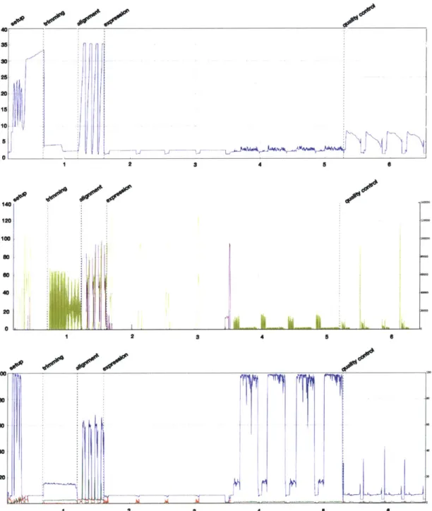
alternative sambamba where possible. An example of the latter is providing parallel implementations of previously existing tools such as GEMINI[128]. Other areas where scalability can break down is in overwhelming the I/O of the machine; we choose algorithms which minimize the amount of I/O they perform and stream as much as possible between steps in the analysis to improve performance. Members of the bcbio-nextgen community have implemented[36] support for collection of performance data in terms of disk I/O and memory, network and CPU usage at each stage in the analysis using collectl[154]. Figure 1-1 on the following page shows an example of the usefulness of collecting these metrics when writing a scalable analysis.
We provide scalability across compute architectures by using the IPython.parallel[133] framework for parallel and distributed computing. We developed the ipython-cluster-helper library to provide a set of abstractions on top of cluster schedulers much like the Distributed Resource Management Application API (DRMMA). DR-MMA provides a unified API for submitting jobs to an array of cluster schedulers but has the limitation that you must have a scheduling system installed on the compute environment. ipython-cluster-helper expands the possible compute configurations
by allowing machines to work as an ad-hoc cluster with no cluster scheduler, as long
as the machines can be accessed via secure shell (SSH). ipython-cluster-helper provides a view to a cluster of machines which uses a simple unified interface to distribute jobs to the cluster of machines. This allows our pipeline to distribute jobs
000-00 0#
40 251iE
F
140 120 20 0 N~ Tf~ U ~ThJ~ 2I
3 2 S 4 4 5 5 a a-
*4$~~__
_
00 20AT~
2 3 4 5Figure 1-1: collectl benchmarks of memory, disk and CPU usage during a RNA-seq analysis. top) memory (in gigabytes), middle) disk (in kilosectors/second, yellow is reads, purple is writes) and bottom) CPU (in percent CPU usage). Having benchmark statistics for each step in the analysis helps when optimizing performance. For example, the period of low CPU usage in this run during expression was due to DEXseq running serially; fixing this and running DEXseq in parallel cut the time to estimate transcript expression in half. Similarly the disk intensive portions during trimming were eliminated by moving to streaming between the trimming steps, (see Figure 1-6 on page 36).
-- --- -I i so
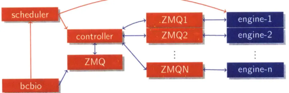
across a wide array of compute architectures; running on a laptop in local mode or running across a cluster with thousands of computers both use the same interface to distribute work. Figure 1-2 shows a schematic of the IPython.parallel architec-ture that ipython-cluster-helper uses for performing parallel computations. An IPython cluster is spun up consisting of a controller process and a set of IPython engines running on arbitrary nodes of a compute architecture. The controller acts as a scheduler, distributing jobs to be run on worker engines. Communication between the controller and the engines happens over ZeroMQ message queues; the controller places a job to be run in the form of a serialized Python function onto a ZeroMQ queue and the worker unserializes the function, runs it locally, saves the result and places a serialized version of the result back on the message queue.
ZMQ1 enlgin~e-1
. .ole ZMQ2 engin11e-2
Figure 1-2: Schematic of parallelization abstraction provided by ipython-cluster-helper.
For each step in the analysis an IPython.parallel cluster is set up using ipython-cluster-helper, consisting of a controller process which distributes the computation and a set of worker processes called engines which perform the computation. The controller is controlled via a client process, in this schematic bcbio. Communication between the client, the controller and the engines occurs over ZeroMQ message queues and require only that a port be open for two-way commmunication between the components of the IPython.parallel cluster. This allows for the compute layer to be abstracted away so that bcbio-nextgen can work with a simple interface to the compute.
ipython-cluster-helper is not limited to use in bcbio-nextgen, it can be used to run any Python program in parallel across all cluster schedulers. Below is an
20 1.1. BACKGROUND
example Python code listing showing ease of taking a simple non-parallel program and parallelizing it using ipython-cluster-helper. This library has been used in other projects that required scaling across multiple machines[128].
Listing 1.1: Parallelizing a serial function with ipython-cluster-helper.
from clusterhelper.cluster import clusterview
from yourmodule import longrunning_function import sys
if __name__ == main__:
# serial version
for f in sys.argv[1:]: longrunning_function(f)
# parallel version with ipython-cluster-helper
with clusterview(scheduler="lsf ", queue="hsph", num_jobs=5) as view:
view.map(longrunning_function, sys.argv[1:])
All of the scalability in the world is useless if the analysis infrastructure is not able
to be relocated to the compute. Thus having a highly scalable pipeline also requires having a pipeline that is easily relocatable and that means having an installation process which installs everything that is necessary for an analysis. This includes all of the necessary data including the genome sequences and metadata about the genome sequences including annotation of gene boundaries and other genomic fea-tures of interest. It also involves installing the correct versions of hundreds of tools, libraries and other programs to run the analysis. These tools have to be installed whether or not the user has administrative access to the machine as many researchers using shared compute environments will not have administrative access. We handle
installation by contributing back to two major projects for installing bioinformatics tools, the cloudbiolinux[2] project and the Homebrew project. Both projects pro-vide simple to specify formula for getting and installing tools on UNIX and MacOS machines. bcbio-nextgen uses these two projects to compile and install the tools necessary to run an analysis.
The combination of abstraction of the underlying compute with
ipython-cluster-helper and the ability to install all of the necessary tools in an environment-agnostic
way allows bcbio-nextgen to be able to easily installed and run in a wide variety of compute environments. Recent work on bcbio-nextgen by Brad Chapman and John Morrissey, in collaboration with groups at Biogen, AstraZeneca and Intel have implemented two extremely useful scalability features in bcbio-nextgen. The first is enabling bcbio-nextgen to be run using the container system Docker[8]. Rather than running the installation script to install all of the tools, installation requires just downloading a Docker container with bcbio-nextgen and all of the dependencies already installed. The second scalability feature is a set of tools to use the Docker images to run an analysis on Amazon Web Services (AWS), pushing and pulling data from Amazon's storage solution, S3. This is an example of one of the major benefits of working on an open source, community driven project: infrastructure like Docker and AWS support only needs to be implemented once for all analyses to take advantage of it. Since the analysis is abstracted away from the compute architecture
it also means rerunning an old analysis can be done on more modern hardware or by other researchers to reproduce an old result.
1.1.5
Reproducibility
High throughput genomics has come under scrutiny in the past couple of years for having issues with reproducibility. Here, our definition of reproducibility is broad; we do not mean reproducing the exact numerical result of an analysis but reproducing the major finding of a paper. Even with this relaxed definition, many genomics experiments cannot be reproduced. This problem is so widespread that the NIH has undertaken an initiative to enhance reproducibility in genomics[40]. One pressing issue is there are often no standards for experimental design or analysis[104], and this is especially true for gene expression experiments. The lack of community derived standards results in widespread reproducibility problems with both microarray[50] and RNA-seq experiments[124].
For an informatics analysis to be reproducible, more than just the data has to be made available. Complete recounting of the command lines of all software, the versions of all software, the versions of all intermediate plumbing type code and code generating the downstream summary statistics must be provided. Not only must this software be made available, it must have to work in the compute environment of the person reproducing the analysis. To be reproducible, the code generating the results must be open; a description of the algorithm is not sufficient to reproduce the results of the code[77]. We address this problem of reproducibility in several ways. The first is that we install all third party tools needed to run an analysis on a wide variety of computing platforms. This allows a person attempting to reproduce results to start from the same base environment. The second is that we record all versions of all third party tools and all command lines run so that an analysis can be reproduced by running the commands if necessary. The third is that if an analysis is run via Docker, a Docker container that contains everything necessary to reproduce
1.1. BACKGROUND
an analysis pre-installed which can be run on a local cluster computer or on Amazon. Each version of a container is specified by a unique id which can be accessed later, meaning an analysis can be completely reproduced by any researcher able to use Docket containers at a later time. The Docker and'AWS implementation in bcbio-nextgen further expands reproducibility, since with that integration a researcher only needs to pay Amazon for the compute and storage and can rerun a published analysis on their own. In these ways, bcbio-nextgen provides a solution to the
reproducibility problem.
1.1.6
Configuration
RNA-seq analyses are complex in part due to a wide array of choices that one can make regarding how the RNA is extracted, how the libraries are prepared, how the sequencing is performed, what organisms are being studied, if the libraries are stranded or not or aimed at tagging a specific portion of a transcript instead of the entire transcript. Each of these options has an effect on the downstream analysis. For example a stranded experiment must take the strand information into account when aligning, quantifying and assembling the reads, so each tool that is run must have the appropriate options set. We provide a carefully considered set of high level options that describe a RNA-seq experiment that an experimenter must set with many of the low level configuration options for each tool set to appropriate default values or appropriate values learned from the data. In this manner we simplify setting up a RNA-seq analysis down to setting a minimum set of parameters that can drive a wide variety of tools underyling the analysis.
These parameters describe whether the library is strand specific or not, which kit was used to produce the library, and which genome the library was from. Parameters
controlling expensive, optional analyses such as whether or not to call variants or assemble the transcriptome can be enabled if those were part of the design of the experiment. We also handle a difficult type of experiment that is often used in cancer research, where a tumor from one organism is grown in another organism, often a human tumor in mouse tissue. When the tumor is sequenced, some mouse tissue can be included. There is an option to disambiguate reads of two organisms in order to remove this type of contamination. Finally, arbitrary metadata about each sample can be provided, such as which batch it is from, if it is treated or not, anything the user can provide. During downstream analyses, this metadata is automatically made available for model fitting and differential expression calling in a separate RNA-seq reporting tool we created called bcbio.rnaseq.
1.1.7
Quantifiable
It is important to have validation datasets for an analysis, both to benchmark the speed of the analysis as well as validate the results of the analysis. Validation datasets allow for an analysis to be fine tuned in terms of new tools or configuration of existing tools to improve results without fear of introducing errors into the data. More importantly it also places the downstream results in a greater experimental context. A validation data set allows a researcher to understand where they are making mistakes or where the analysis is blind and can help guide downstream users of the data towards the most salient results.
Having a standardized, quantifiable analysis allows a researcher to treat their analysis as an optimization problem and improve it. Benchmark data sets serve as type of integration test for the software making up an analysis pipeline. When a new tool is published, it is standard for the work to show a comparison to the standard
tools of the day and show how the new tool outperforms the old in some aspect. Occasionally review papers compare several tools to each other with a validation dataset to determine in a less biased way the strengths and weaknesses of each tool[98][144]. These papers are valuable but often there has been no fine tuning of any of the comparison algorithms. Consequently, they are often run with their default values and are compared against each other, whereas a researcher with experience with a particular tool would be able to tune it to get better results. bcbio-nextgen is tool agnostic and tools have gone through a process of fine tuning the configuration parameters already. Tools are chosen based on the consensus of the users regarding which tool works best and the tools are tuned or improved to give the best results. This allows for a fair comparison across tools when evaluating making changes to an analysis pipeline.
In addition to being tool agnostic, bebio-nextgen is also dataset agnostic. If a new benchmark dataset comes out for a particular aspect of a pipeline, the cor-rect values for the benchmark dataset can be added and the benchmark dataset run through the pipeline and compared. In this way researchers can improve both the analysis itself and the measurement of the analysis simultaneously through the incorporation of new benchmark datasets.
Researchers can ask many more questions of their RNA-seq data than with mi-croarray analyses. Expression can be summarized and differential expression called at the gene, transcript, exon and splicing event level. Rearrangements and variants, gene fusion events and RNA-editing events can all be assayed with RNA-seq. Novel genes and novel isoforms can be assembled, and differential usage of promoter sites can be analyzed. Each of these aspects of an analysis have several tools which handle them and each needs a benchmark dataset to test against when testing iterations of a pipeline. bcbio-nextgen gathers available benchmark datasets from the
nity to test each aspect of RNA-seq analysis. We provide benchmark datasets in the form of data from actual experiments and simulated data to benchmark gene-level and transcript-level expression calling, transcriptome assembly with and without a reference data set and fusion gene calling on cancer datasets. As the community develops alternate benchmarks we fold them into bcbio-nextgen.
Gene and transcript expression
bcbio-nextgen uses a combination of validation datasets from real data and
simu-lation to assess the results of the gene-wise differential expression analysis. The first validation dataset is from phase three of the Sequencing Quality Control (SEQC) [41] project from the US Food and Drug Administration. The goal of releasing these datasets was to provide laboratories with known reference standards to use to tease out the types of technical variation introduced across laboratories, sequencers and protocols. This dataset consists of a two sets of samples: the first is RNA sequenced from the Universal Human Reference RNA (UHRR) from Agilent. This sample is composed of total RNA from ten human cell lines to be used as a reference panel. The second sample is from the Human Brain Reference RNA (HBRR) panel from Ambion which consists of brain samples from all regions in several subjects pooled together to form a reference panel. The SEQC project provides qPCR results from one thousand genes in the UHRR and HBRR panels, to serve as a proxy for a truth dataset. The validation dataset we analyze is fifteen million randomly selected reads from five replicates of each SEQC sample.
The SEQC data have a few major limitations as a validation data set. The first limitation is that since the RNA comes from stock of pooled RNA, the replicates are technical replicates of only the library preparation and sequencing and do not take
into account variability induced by RNA-extraction or biological variability such as samples from different mice or humans. Proper handling of biological variability is important component in a RNA-seq analysis and the SEQC dataset is not an appropriate way to assess it. The second major limitation is that the validation data is gene-level qPCR data. RNA-seq data is capable of assessing expression at the level of the transcript but the SEQC data set will not be useful for assessing quantitation at anything other than the level of the gene.
To address these limitations the we also produce simulated datasets of raw RNA-seq reads using Flux Simulator [67], an in-silico RNA-RNA-seq experiment simulator. Using Flux Simulator, reads are generated from a given reference transcriptome and many steps and biases introduced during RNA-seq library preparation are simulated in-cluding fragmentation at the RNA or cDNA level, reverse transcription, PCR ampli-fication, gene expression and sequencing. Flux Simulator does not produce biological replicates, so we implemented a simulator to add biological noise and fold change spike ins to the data generated by Flux Simulator to mimic biological replicates and differential expression in a real experiment. This package is available online as
flux-replicates.
RNA-seq count and read simulator
Flux Simulator outputs a simulated relative expression level, p which is the pro-portion of the total RNA molecules in the simulated sample that are from a given transcript. These values are used as a baseline level of proportions from which a sin-gle factor differential expression experiment is simulated by spiking in fold changes between replicates of a sample. We implemented a RNA-seq read count simulator[94]
by setting a proportion of the simulated transcripts to be differentially expressed at
range of fold changes and drawing counts for each gene from the negative binomial distribution with the dispersion parameter set to increase as the expression level decreases, to mimic real data(Figure 1-3 on the following page).
Starting from a given level of biological coefficient variation, BCV, a relative expression level for gene y with proportion of the total expression level py and a library size
1
for a sample, we simulate cy, the counts of transcript y from the negative binomial distribution by composing a gamma distribution and a poisson distribution to add biological and technical noise, respectively:Py =
Py
(1.1)BCVy = (BCV+ I
)
Vx)
2(
40)
(1.2)
CY ~ T(B(pty, BCVy))
(1.3)
B is a function that draws values from a gamma distribution of mean Py and
vari-ance BCVY2 and T draws values from a poisson distribution with mean B(py, BCVy). We add random noise dependent on expression level of the gene to BCV to simulate the higher dispersion of the negative binomial at low counts (figure 1-3 on the next page).
The simulator can be run in a mode where it is supplied with an existing set of counts from which the parameters for the simulation are estimated to match the existing data. This allows the user to take a previously run experiment and estimate what would happen if they sequenced less reads or changed the number of replicates. It also allows for some rough post-hoc power calculations to inform future experimental design choices and to make stronger negative result claims rather than failing to reject the null hypothesis of no differential expression.
1.1. BACKGROUND I 00000000 C 1000000-1004 0 * gO 0
7-Sb *060; 10 1000 100000 mean count
Figure 1-3: The Poisson distribution is overdispersed for RNA-seq count data. Variance vs. mean counts for a RNA-seq experiment (black dots) with variance estimated by the Poisson (black line) and negative binomial (blue line) distributions. Each point on this graph is the mean and variance for a single gene across biological replicates. RNA-seq data is more noisy than expected from the Poisson due to additional technical and biological variability.
As an example, RNA sequencing is very expensive and time consuming and often experimenters are looking to maximize the power of their experiment and minimize the cost. One potential optimization involves determining how many reads to
se-quence against how many replicates to run. An experiment running at most on two HiSeq lanes can expect at least 300 million reads. This leaves a case-control experi-ment with three replicates at 50 million reads per sample. Alternatively, rather than sequencing six samples at 50 million reads per sample, the read depth could be cut in half and twice as many replicates could be sequenced. Using the simulator to compare these two experiments against each other, we can make a recommendation to run more replicates at lower depth if the goal is to identify differentially expressed genes at moderate-to-high fold change (Figure 1-4 on the following page). In addi-tion, if the genes of interest are at the low end of the differential expression spectrum, we could recommend to not run the experimental at all.
1.1.8
RNA-seq implementation
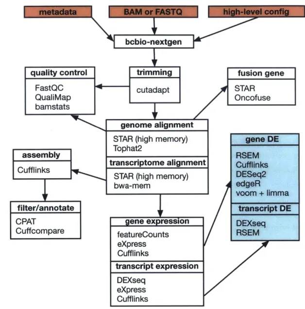
Figure 1-5 on page 34 shows a high level overview of the RNA-seq pipeline imple-mented in bcbio-nextgen version 0.8.5a. The implementation covers quality control of the data, adapter sequence removal, aligning to the genomes, quantifying at the gene, isoform and exon level, calling variants and RNA-editing events, transcriptome assembly, classification and filtering and calling differential expression events at the gene, isoform and exon level using several commonly used tools. There are a mul-tiplicity of third party tools that could be used to perform each step and tools are chosen based on considering their accuracy, licensing, scalability in terms of CPU, IO or memory bottlenecks and how well they are actively maintained. When compute constraints may be a roadblock, alternatives are provided; for example the STAR[48]
1.1. BACKGROUND 32
1.05
.1to
4OO-
zoo-200 ---IIII
0 i_h
I
edgeR Voomkimma (a) 4W-~400-
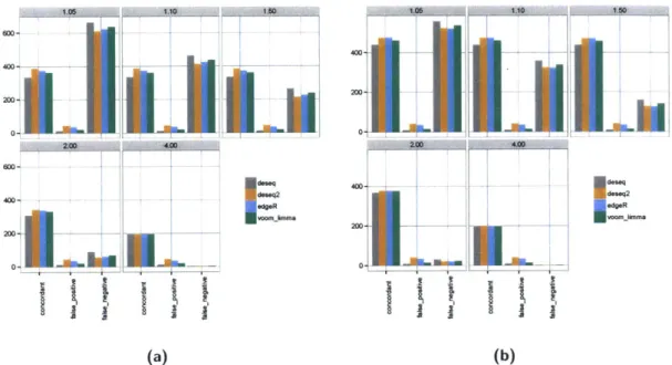
edgeR voomlmm -1 -L-(b)Figure 1-4: RNA-seq differential expression concordance calculation from two simulated experiments. An RNA-seq experiment was simulated with a sample size of three and a library depth of 50 million reads (a) and a sample size of six and a library size of 25 million reads (b). We simulated 200 genes as differentially expressed up or down across each of five fold changes: 1.05, 1.10, 1.50 and 4.0. Each facet of the graph calculates concordance, false positive an false negative rate, considering only genes at the specified fold change or greater. Four commonly-used negative binomial based differential expression callers (DESeq2[101], DESeq[6], edgeR[149] and limma[94]) were run on the data and their concordance with the known fold changes from the spike ins were simulated. At large fold changes most of the spike in genes are correctly called differentially expressed in both experiments but at fold changes below four, the experiment with a higher number of replicates calls more concordant differentially expressed genes.
aligner, while very fast and accurate has a large memory requirement which may make it not feasible to use in some compute environments. In that instance a slower, less memory intensive alternative in Tophat2[170] is offered (see Figure 1-5, align-ment box). In the following sections a brief, non-comprehensive rationale behind choosing the tools for each step in the analysis is covered. Where appropriate there is a discussion of optimizations we implemented to improve the accuracy and speed of the chosen tools. This discussion isn't intended to be an exhaustive comparison of every tool for each step or a conclusive statement about which tools are better than others, but more a breakdown of the tradeoffs, possible pitfalls and other im-portant considerations for each step in the analysis. The design philosophy of the bcbio-nextgen RNA-seq pipeline implementation is to use the data to tune as many parameters as possible to optimize for the particular data set being processed while maintaining a balance between accuracy and throughput and the tool choices reflect
that philosophy.
Read trimming
RNA-seq reads can have contaminating sequences at the ends of the reads in the form of adapter sequences, poly-A tails or other sequences, which may cause issues during alignment or in downstream analyses, resulting in loss of information. Some spliced-read aligners such as STAR will handle these spliced-reads by soft clipping the homopolymer or adapter sequences that don't align to the genome but other aligners such as Tophat do not handle these reads well. For RNA-seq, adapter contamination on the ends of reads can often be a problem; under most library preparation protocols the RNA is fragmented before conversion to cDNA and there may be small pieces of RNA for which the read length is longer than the fragment. For these small RNAs with long
1.1. BACKGROUND 34
bcbio-nextgen_
quality control
trimming
FastQC
cutadapt
QualiMap
p
bamstats
V~K
4
genomealignment
assembly
Cufflinks
filter/annotate
CPAT
Cuffcompare
STAR (high memory)
Tophat2
transcriptome alignment
STAR (high memory)
bwa-mem
gene expression
featureCounts
eXpress
Cufflinks
transcript expression
DEXseq
eXpress
Cufflinks
Figure 1-5: Schematic of RNA-seq analysis. A high level overview of the implementation
of the RNA-seq pipeline in bcbio-nextgen version
0.8.5a,
with the external programs used in each module listed. Included are modules to do gene, isoform and exon-level differential expression calling, variant calling on RNA-seq data, fusion gene calling for assaying structural variation in cancers, transcriptome assembly, quality control of the raw data and the alignments, clustering and sample outlier detection and automatic report generation. Red colored boxes indicate user-supplied data and green boxes are functionality supplied by bcbio.rnaseq.fusion gene
STAR
Oncofuse
gene DE
RSEM
Cufflinks
DESeq2
edgeR
voom + limma
transcript DE
DEXseq
RSEM
1.1. BACKGROUND 34read lengths, the read will be long enough to continue on past the RNA sequence into the adapter sequence. Several tools that have been created to fix this adapter read through issue, with tradeoffs regarding specificity, sensitivity and speed[83].
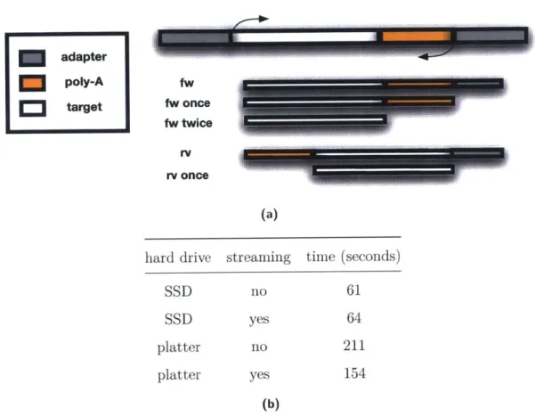
Careful tuning of the parameters of the read trimmer beyond the default values can improve sensitivity and specificity. Figure 1-6a on the following page shows that tuning cutadapt[109] to trim twice on the forward reads, once to trim possible adapter read-through and once to trim polyA sequences that are masked by the adapter sequence can rescue reads that would have been lost from the 3' end of RNAs. Beyond tuning for accuracy, paired-end read trimming using cutadapt can be tuned to run faster on compute environments with spinning disks by a simple architecture change. When run in paired-end mode, cutadapt must write two temporary files to disk and be run twice, this I/O operation is very slow and takes time. If running thousands of samples simulataneously, this can become a large bottleneck in an analysis. If instead of writing temporary files to disk, the command is constructed to use named pipes[164] instead, a 30% gain in performance can be realized, even on a very small dataset of a single lane of a million reads.
There has been some debate regarding if it is useful to trim low quality ends of reads before aligning. Most, but not all, modern aligners can take into account the low quality scores so most analysis pipelines include a quality trimming step. The commonly used threshold for RNA-seq is to to trim bases with PHRED quality scores less than 20, but a more gentle threshold of 5 results in much less information
1.1. BACKGROUND 36 fw fw once fw twice rV rv once (a)
hard drive streaming time (seconds)
SSD
SSD
platter platter no yes no yes 61 64 211 154 (b)Figure 1-6: Tuning of adapter trimming with cutadapt. a) Trimming of adapter, polyA tails and other non-informative contaminant sequences from the ends of reads is necessary for compatibility with downstream tools that cannot handle reads with contaminated ends, such as aligners that do no soft clipping or kmer counting algorithms. cutadapt needs the flag set to try trimming twice when handling RNA-seq data to be able to trim polyA tails masked by adapter sequence. b) cutadapt requires intermediate files to be written out when handling paired end data and cannot natively stream the files from one step to another. For small amounts of data on fast disks (SSDs), this does not contribute to the processing time at all. On slow disks writing the intermediate files is the bottleneck in the process. Replacing the intermediate files with named pipes, thus re-enabling streaming, speeds up processing by 30% on a million paired-end reads.
adapter
poly-A
target
Alignment
RNA-seq reads may cross exon-exon boundaries and when aligned to the genome will appear to be split across an exon. RNA-seq aligners have to be split-read aware or be able to take a gene model and create a proper alignment for these reads. The STAR aligner[48] is very fast and accurate aligner for RNA-seq that can map reads up to 50 times faster than Tophat2 but requires a machine with 50 GB of memory to run[54]. In addition to mapping reads quickly and accurately, STAR can simultaneously generate a mapping to the transcriptome for use with downstream quantitation tools such as eXpress[146], saving a step in the downstream analysis.
When high-memory compute is not available, Tophat2 is run instead of STAR. For paired-end reads, a small subset of the reads are mapped with Bowtie2 to determine an estimate of the mean and standard deviation, using the median and median absolute deviation as proxies for the mean and standard deviation of the insert size. The transcriptome-only mapping is made using bwa-mem since there is not a need to handle the intron spanning reads and bwa-mem is extremely fast and sensitive.
Transcriptome expression quantification
The primary goal of most RNA-seq experiments is to examine differences in the transcriptome between two or more experimental conditions. In order to assay the differences in transcription, the transcriptome must first be quantified. Depending on the organism, quantifying the expression of the transcriptome can be more com-plex than it initially seems. In organisms that have little to no alternative splicing of transcripts, this task is conceptually simple: count up the number of reads map-ping to each gene and determine if the number of reads mapmap-ping to the gene is systematically different between conditions. For organisms such as the human with
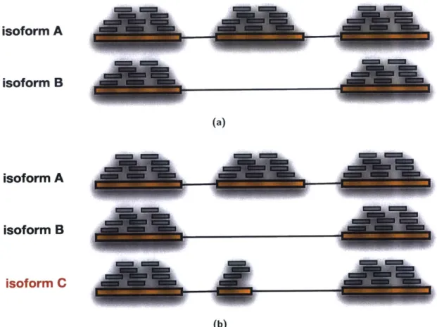
transcriptomes that undergo intensive alternative splicing[181], the task of calling dif-ferences between conditions is much more complex. The complexity arises because what is sequenced are small pieces of transcripts which, when alternatively spliced, can be very similar to each other. Figure 1-7 on the next page shows an example where a single gene has multiple transcripts. Determining which isoform to assign reads that could come from multiple transcripts is a complex chicken-and-egg prob-lem since it requires knowledge of how much of each transcript is expressed, which is what you are trying to estimate.
Many approaches ignore the read assignment issue altogether by quantifying at the level of the gene; the reads aligning to all transcripts of a gene are counted and combined to be the total reads mapping to the gene. The trouble with this approach is it doesn't reflect reality, the reads came from individual transcripts, not a gene and quantifying expression in this way can lead to errors. Figure 1-7 on the following page shows an example of one type of error, where a splicing event results in the expression of a much smaller transcript in one condition resulting in a false differential expression call.
Other practical concerns make quantifying the expression of the transcriptome difficult. Quantifying transcripts is dependent on the state of the annotation of the transcriptome because isoforms of genes that do not occur in the transcriptome will not have reads assigned to them, and reads that were sampled from unannoted isoforms will be misattributed to related isoforms, an issue illustrated in cartoon form in Figure 1-7 on the next page. The state of the transcriptome annotation for model organisms varies widely even for closely related organisms that should show similar degrees of alternative splicing (e.g. Figure 1-8 on page 44). Thus, for most organisms, augmenting the existing transcriptome assembly is necessary for accurate differential isoform calls. However this thesis, (Table 1.1 on page 43) and work of
isoform A
isoform B
(a)isoform A
isoform B
isoform C
(b)Figure 1-7: Gene level quantification can introduce errors. a) Quantification at the gene level can introduce quantification errors. If in one condition isoform A is expressed and in another condition isoform B is expressed, quantification at the gene level by counting the number of reads aligning to each gene will show a 1.5x fold change, even though the expression of the gene is unchanged. b) Missing isoforms can introduce errors in isoform-level differential expression calls. In the illustration, isoform C is missing from the annotation which will lead to reads being incorrectly assigned to isoform A. This also illstrates the complexities of assigning reads to specific isoforms; if a read aligns to the first exon, determining to which transcript of the gene it should be assigned is not a trivial problem.
others[3] have shown that transcriptome assembly is often incomplete and rife with false positives. Including these error prone assemblies introduces a major source of noise and into quantifying the transcriptome expression.
The challenges in quantifying at the isoform level have lead to the exploration of algorithms quantitating individual splicing events, exons and parts of exons instead of isoforms[87][7]. Quantitating at this level requires much less accurate transcrip-tome information and only requires enumeration of the exons and splicing events that can occur in the data, a much more tractable problem than a complete enumer-ation of all possible isoforms. In addition, for incomplete transcriptome annotenumer-ations, assembling exons is much more successful than assembling entire isoforms[3], espe-cially for organisms in which splicing is complex, and the enumeration of the exons is generally more complete in exisiting transcriptome annotations. Recently a method called derfinder[60] was developed which takes the resolution of the transcriptome quantitation to the extreme and quantitates transcriptome expression at the level of a single base.
Transcriptome quantification is implemented at three levels of resolution in
bcbio-nextgen, at the level of the gene with featureCounts[97], eXpress[146] and Cufflinks[172],
the isoform level with eXpress and Cufflinks and the sub-exon level with DEXseq[7]. featureCounts and eXpress both generate gene-level estimated counts of reads map-ping to genes, suitable for use in count-based differential expression callers (see Sec-tion 1.1.8 on the following page); featureCounts only counts reads which can be uniquely assigned to a gene whereas eXpress assigns ambiguous reads probabilisti-cally based on the overall expression of the gene. There are other tools with similar functionality to featureCounts and eXpress, but featureCounts and eXpress are both extremely fast, up to 30 times faster than similar tools[97]. For isoform expression, both eXpress and Cufflinks produce estimates of the gene-level and isoform level
expression, eXpress summarizing with estimated counts suitable for use in count-based callers and Cufflinks with FPKM, a gene-length normalized expression mea-sure, which a companion program Cuffdiff uses to call differential isoform expression. Finally DEXseq quantitates differential expression at the level of the exon fragment; exons are broken into the smallest fragments unique to an isoform in the existing annotation and DEXseq quantitates the expression of those fragments. Each of these levels of quantitation are used to make differential expression calls in a com-panion tool released with bcbio-nextgen, bcbio.rnaseq, this gives the researcher flexibility to choose the resolution of quantitation that is most appropriate to their experiment.
Differential expression
Differential expression calling on the gene, isoform and splicing event level is per-formed with a companion program to bcbio-nextgen called bcbio.rnaseq. bcbio.rnaseq runs baySeq[72], DESeq2[101], edgeR[149], Cufflinks[171], voom+limma[94], edgeRun[47] and EBSeq[95] to call gene-level differential expression, Cufflinks and EBSeq to call isoform-level differential expression and DEXSeq to call splicing event level differ-ential expression using the estimated expression values calculated from the bcbio-nextgen RNA-seq pipeline. Running several tools is important, as different tools perform well on specific types of RNA-seq data. DESeq2 and limma are great choices for most RNA-seq experiments, but they can be outperformed in specific conditions. For example for low replicate, low count experiments with under ten million reads per sample or less, we have created an improved algorithm called edgeRun[47], which is much more sensitive for these specific types of experiments.