HAL Id: tel-03150015
https://tel.archives-ouvertes.fr/tel-03150015
Submitted on 23 Feb 2021
HAL is a multi-disciplinary open access
archive for the deposit and dissemination of sci-entific research documents, whether they are pub-lished or not. The documents may come from teaching and research institutions in France or abroad, or from public or private research centers.
L’archive ouverte pluridisciplinaire HAL, est destinée au dépôt et à la diffusion de documents scientifiques de niveau recherche, publiés ou non, émanant des établissements d’enseignement et de recherche français ou étrangers, des laboratoires publics ou privés.
rolling tire with refracted PIV method
Damien Cabut
To cite this version:
Damien Cabut. Characterisation of the flow in a water-puddle under a rolling tire with refracted PIV method. Other. Université de Lyon, 2020. English. �NNT : 2020LYSEC025�. �tel-03150015�
THÈSE de DOCTORAT DE L’UNIVERSITÉ DE LYON
opérée au sein de l’École Centrale de Lyon
École Doctorale N
◦162
Mécanique Énergétique Génie Civil Acoustique Spécialité de doctorat : Mécanique des Fluides
Soutenue publiquement le 13/10/2020, par Damien Cabut
Characterisation of the flow in a water-puddle under a rolling
tire with refracted PIV method.
Devant le jury composé de:
Bruecker, Christoph Professeur City University of London Rapporteur
Vetrano, Maria-Rosaria Professeur Katholieke Universiteit Leuven Présidente du jury
Gabillet, Céline Maître de Conférences Ecole Navale Examinateur
Todoroff, Violaine Docteur Michelin Examinateur
Simoens, Serge Directeur de recherche École Centrale de Lyon Directeur de thèse
Résumé :
L’écoulement au sein d’une flaque d’eau lors du passage d’un pneumatique en roulement est étudié dans ce travail. Une méthode de mesure adaptée aux mesures sur piste sous un véhicule en roulement est développée dans un premier temps. Cette méthode basée sur la méthode PIV (Vélocimétrie par Images de Particules), consiste en la réfraction de la nappe laser à l’interface hublot/écoulement afin de pouvoir éclairer les particules par le même accès optique que la collection d’images. Cette technique appelée refracted PIV (R-PIV) est caractérisée dans un premier temps sur un écoulement contrôlé en laboratoire. Cette technique est ensuite adaptée au cas de la piste pour les mesures in-situ. Ces mesures appliquées à la piste ont permis de mettre en évidence différents comportements de l’écoulement dans la flaque d’eau en amont du pneumatique mais également au sein des sillons pneumatiques. En amont du pneumatique les évolutions linéaires de la vitesse du fluide en fonction de la vitesse du véhicule est mise en évidence dans ce travail. Des effets non linéaires sont égalements observés et mis en lien avec la réduction de l’aire de contact pneu chaussée. Dans un second temps, l’étude de l’écoulement au sein des sculptures du pneumatique dans l’aire de contact nous permet de mettre en évidence deux grands types de sculptures. Le premier est composé de tous les sillons longitudinaux du pneumatique. Dans ces sillons, la vitesse de l’écoulement à travers ces sculptures dépend de la vitesse véhicule mais également de la présence du témoin d’usure du pneumatique. Un écoulement secondaire tourbillonnaire a également été mis en évidence grâce à nos mesures sur piste. Dans le second type des sillons composés de toutes les sculpures orientées transversalement, la vitesse du fluide, en leur sein, dépends de leur position dans l’aire de con-tact. Cette évolution semble être fonction de la déformation du pneumatique dans l’aire de concon-tact. Pour finir, les intéractions entre ces différents types de sculptures sont également discutées dans ces travaux permettant d’expliquer certains comportements spécifiques.
Mots Clés : Vélocimétrie par Images de Particules (PIV), Réfraction, Pneumatique, Hydroplanage, Ecoulements multiphasiques, Surface Libre.
In this work, the fluid flow in a water puddle while a rolling tire crosses the puddle is studied. A mea-surement method adapted to track meamea-surements under a rolling tire is developed. This method, based on PIV (Particle Image Velocimetry), is based on the refraction of the laser light sheet at the flow/window interface. This allows us to illuminate particles and record their images from a single optical access. This technique called refracted PIV (R-PIV) is characterised with a laboratory controlled experiment. When characterised, this technique is applied to in-situ measurements on the track. Measurements performed allow to highlight specific behaviours in different parts of the flow, in front of the tire and inside tire grooves in the contact patch area between the tire and the road. In front of the tire, the linear evolution of the water velocity in the puddle as a function of the vehicle speed is demonstrated. At high vehicle speed, non-linear effects are highlighted and linked to the shape of the contact patch area which evolves at high vehicle speed. Under the tire contact patch area, two main types of grooves contribute to the draining of water. Firstly, the longitudinal grooves are the straight grooves aligned with the rolling direction. In these grooves, the velocity of the fluid flow depends on the vehicle speed and also on the presence or not of the wear indicator. A secondary vortex like flow structure is also demonstrated in this work. The second type of grooves are the transverse grooves which are the grooves oriented with a certain angle compared to the car rolling direction. In these grooves, this work proved that the velocity is dependent on the groove location in the contact patch area. This seems to be linked to the tire deformation with the load of the car in the contact patch area. Finally, this work discussed the link between the different tire groove types to explain different specific behaviours.
Key words : Particle Image Velocimetry (PIV), Refraction, Tire, Hydroplaning, Multiphase flow, Free-surface.
Cette thèse a été réalisée dans le cadre d’un projet FUI (Hydrosafe tire) financé par BPI France (n◦ DOS0051329/00) et la région AURA (n◦ 16 015011 01). Les partenaires de ce projet étant le Labora-toire de Mécanique des Fluides et d’Acoustique (LMFA) de l’Ecole Centrale de Lyon, le LaboraLabora-toire d’Hydrodynamique, d’Energétique et Environnement Atmosphérique (LHEEA) de l’Ecole Centrale de Nantes, Nextflow Software et Michelin.
Je souhaite tout d’abord remercier mes encadrants de thèse pour leur soutien tout au long de ma thèse. Merci à Serge pour la gestion de la thèse et pour m’avoir fait confiance pour ces 3 années. Merci à Marc pour l’aide apportée tout au long de la thèse. Je souhaiterai également remercier les collaborateurs du projet de Centrale Nantes et de Nextflow ainsi que les partenaires de Michelin. Je souhaite tout particulièrement remercier Violaine pour sa disponibilité et les sessions manips à Ladoux avec Jean. Je voulais de plus remercier Loïc pour son aide en optique et Nathalie pour sa disponibilité pour la gestion des ressources.
Je tiens à remercier tous mes collègues doctorants et post-doctorants pour les discussions construc-tives ou non du midi et les parties de babyfoot endiablées. Je ne me lance pas dans une liste par peur d’oublier quelqu’un mais ils se reconnaîtront. Mention particulière à Yann et Simon pour les petits repas et le tour des restos lyonnais.
Un grand merci également à ma famille et mes amis pour le soutien morale tout le long de ma thèse. Merci à la bande de Puffer pour les instants détentes et la présence pendant la soutenance.
Une petite pensée en la mémoire de Jean-Pierre Hermand qui m’a pris sous son aile pour mes 7-8 mois de stage de recherche à Polytechnique Bruxelles pour ma première expérience en labo de recherche.
1 Introduction and State of the Art 20
1.1 Context and Motivations. . . 20
1.2 Analysis of the flow in a puddle with a rolling tire. . . 22
1.2.1 Experimental studies of the phenomenon. . . 22
1.2.1.1 Visualisation of the Contact patch area. . . 23
1.2.1.2 Velocity measurements in presence of water . . . 24
1.2.2 Some Numerical studies of the hydroplaning phenomenon. . . 24
1.2.3 Purpose of this work. . . 25
1.3 The flow structure. . . 26
1.3.1 Different zones of the flow. . . 26
1.3.2 Flow in front of the tire. . . 26
1.3.3 Flow in tire groove. . . 27
1.3.4 Conclusion. . . 30
1.4 Thesis organisation. . . 30
2 The refracted PIV (R-PIV) technique. 33 2.1 The Particle Image Velocimetry (PIV). . . 33
2.1.1 planar PIV technique. . . 33
2.1.1.1 Description of a planar PIV set-up. . . 33
2.1.1.2 Description of the cross correlation. . . 34
2.1.2 Microscopic PIV (µ-PIV) technique. . . 36
2.1.2.1 Description of a µ-PIV set-up. . . 36
2.1.2.2 Cross-correlation and integration effect. . . 36
2.1.3 R-PIV a hybrid technique adapted to confined spaces. . . 37
2.2 Experiental set-up for R-PIV testing. . . 38
2.2.1 The bench and operating conditions . . . 38
2.2.2 Emitting Optics . . . 39
2.2.3 Seeding . . . 40
2.2.4 Image acquisition and processing . . . 40
2.3 Optical properties for R-PIV. . . 41
2.3.1 The laser sheet propagation. . . 41
2.3.1.1 Measurement of the laser sheet intensity after the refraction. . . 41
2.3.1.3 Long range propagation for tire application. . . 45
2.3.2 Depth of focus. . . 46
2.3.3 Conclusions. . . 47
2.4 Cross-correlation statistical model for R-PIV . . . 47
2.4.1 Cross correlation model (CCM). . . 47
2.4.1.1 The cross-correlation general form. . . 47
2.4.1.2 Statistical convergence. . . 50
2.4.2 Analysis of the illumination methods with the CCM . . . 53
2.4.2.1 Model Prediction for P-PIV. . . 53
2.4.2.2 Model Prediction for R-PIV. . . 54
2.5 Results and validation of the model . . . 55
2.5.1 Flow Structure. . . 55
2.5.2 R-PIV results. . . 56
2.6 Conclusions . . . 59
2.6.1 Optical properties of R-PIV . . . 59
2.6.2 Prediction of the measured velocity using a cross-correlation model . . . 59
3 Application to tire flow measurements. 61 3.1 Experimental set-up for tire measurements. . . 61
3.1.1 Measurement pit. . . 61
3.1.1.1 2D2C R-PIV measurement set-up . . . 61
3.1.1.2 2D3C Stereoscopic R-PIV measurement set-up . . . 61
3.1.2 Reception Optic. . . 63
3.1.3 Seeding particles. . . 64
3.1.4 Emission Optic. . . 65
3.1.5 Conclusions. . . 68
3.2 Measurement protocol for R-PIV measurements. . . 68
3.3 Tire models studied. . . 69
3.3.1 Primacy 4 (PCY 4) (commercial summer tire). . . 69
3.3.2 Wear state. . . 70
3.4 Coordinate system and contact patch. . . 70
3.4.1 PCY4 tire. . . 71
3.4.2 CCP tire. . . 72
3.5 Flow zones and velocity fields processing. . . 73
3.5.1 In front of the tire. . . 74
3.5.2 Inside tire grooves. . . 74
3.5.3 Repetition strategy and ensemble averaging. . . 75
4 Sources of Variabilities. 77 4.1 Influence of control parameters. . . 77
4.1.1 The water height. . . 77
4.1.2 Vehicle speed. . . 77
4.1.4 Contact patch position. . . 78
4.1.5 Mask positioning. . . 79
4.2 Metrological sources of variabilty. . . 79
4.2.1 In front of the tire. . . 79
4.2.2 Inside tire grooves. . . 80
4.3 Hydrodynamic source of variabilities. . . 81
4.3.1 Transverse grooves position. . . 81
4.3.2 Wear indicator position. . . 82
4.3.3 Turbulence. . . 82
4.4 Conclusions. . . 83
5 Metrological discussion. 85 5.1 Metrological sources of bias in front of the tire. . . 85
5.1.1 Geometry of the flow in front of the tire. . . 85
5.1.2 Fluorescent Particle motion in the fluid. . . 86
5.1.2.1 Falling time before acquisition. . . 87
5.1.2.2 Particle behaviour submitted to highly accelerated flows. . . 90
5.1.3 Boundary Layer presence. . . 94
5.1.3.1 Mechanisms of boundary layer creation. . . 94
5.1.3.2 Boundary layer and cross-correlation model. . . 98
5.2 Metrological sources of bias inside longitudinal grooves. . . 100
5.2.1 Optical influence of the bubbles in the model. . . 101
5.2.1.1 Single millimetric bubble. . . 103
5.2.1.2 Slab of small bubbles. . . 104
5.2.1.3 Conclusions . . . 106
5.2.2 Cross-correlation model analysis in case of counter-rotating vortices. . . 106
5.2.3 Discussion on the streamwise velocity. . . 110
5.2.4 Conclusions. . . 110
5.3 Illumination in transverse grooves. . . 110
6 Tire R-PIV measurement results. 114 6.1 PCY4 Tire. . . 114
6.1.1 Flow in front of the Tire. . . 114
6.1.1.1 Water-Bank . . . 117
6.1.1.2 Shoulder . . . 118
6.1.1.3 Conclusions . . . 120
6.1.2 Flow inside tire grooves. . . 120
6.1.2.1 Primary flow inside longitudinal grooves. . . 121
6.1.2.2 Secondary flow inside longitudinal grooves. . . 125
6.1.2.3 Flow inside transverse (Type C) grooves. . . 130
6.2 CCP Tire. . . 132
6.2.1 Flow in front of the Tire. . . 132
6.2.1.2 Shoulder . . . 134
6.2.2 Flow inside the grooves. . . 134
6.2.2.1 Flow inside the "zigzag" zone. . . 134
6.2.2.2 Flow inside Type W grooves. . . 136
6.3 Conclusions. . . 138
7 Analysis of the tire flow. 141 7.1 Flow in front of the tire. . . 141
7.1.1 Evolution of the velocity with the vehicle speed. . . 142
7.1.2 Evolution of the water-bank length with the vehicle speed. . . 145
7.1.3 Self-similarity of the flow. . . 147
7.2 Flow in straight grooves. . . 150
7.2.1 Flow in the streamwise direction. . . 150
7.2.1.1 Evolution of the velocity with the Vehicle speed. . . 150
7.2.1.2 Similarity of the profiles. . . 151
7.2.2 Vortex structure of the flow. . . 152
7.2.2.1 Vortices intensity. . . 152
7.2.2.2 Hypothesis on the vortices creation phenomena. . . 155
7.3 Flow in transverse grooves. . . 158
7.4 Interaction of connected grooves. . . 159
8 Conclusions and Perspectives 162 8.1 Major findings. . . 162
8.2 Perspectives. . . 164
A Demonstration of the cross-correlation model calculation. 166
B Image Treatment. 176
C Decreasing interrogation windows size in tire grooves. 179
D The change of object plane position for the flow in the grooves. 182
E Boundary layer in tire groove. 184
1 Sketch of the tire specific vocabulary used in the PhD. . . 18
1.1 Aquaplaning sketch of the 3 different zones. . . 21
1.2 Images obtained for the contact patch determination from Todoroff et al. 2019 [72]. . . . 23
1.3 Scheme of the geometry of the flow in the Hydrodynamic zone (with the three parts highlighted) with the corresponding averaged velocity profile over the water height in z. . 26
1.4 Sketch of the wall-jet in front of the tire. . . 27
1.5 Zoom on tire grooves from Todoroff et al. 2019 [72]. . . 28
1.6 Sketch of the vortices inside the tire grooves from Yeager 1974 [81]. . . 29
1.7 Groove images for both new and worn tires. Upper image is the smallest groove and lower image is the largest groove (from Todoroff et al. 2019 [72]) . . . 30
2.1 Scheme of a light sheet illuminating particles for P-PIV measurements. . . 33
2.2 Scheme of the two images recorded with the interrogation windows represented. . . 34
2.3 Scheme of the decomposition of the cross-correlation function. . . 35
2.4 Illustration of the 3 components contributions to the total cross-correlation. . . 35
2.5 Scheme of he set-up configuration for a µ-PIV experiment. . . 36
2.6 Scheme of the illumination method for velocity measurements inside a liquid film using refraction. . . 37
2.7 a) Scheme of the hydraulic loop with P for the pump and F for the flow-meter. b) Scheme of a cross-section of the channel. c) Picture of the channel mounted on the PMMA block. 38 2.8 Side view of the experimental setup for a) P-PIV, b) R-PIV. In all the following study, x∗= xh, y∗=hy, z∗=hz. . . 39
2.9 Set-up for the in-situ measurement of the inclined light sheet intensity profile. Left picture is a photo of the emerging light sheet. . . 41
2.10 Light sheet profile I0∗(z∗) a) near the beam-waist for P-PIV, b) at x∗= 8 for the R-PIV. . . 42
2.11 Dashed-doted colored lines are planar horizontal light sheets corresponding to z∗sup,z∗max and z∗in f. Purple dotted line is the position of the camera object plane (Fig.2.17). The normalized intensity profile function of the height (right) is also presented to show the correspondence between limit lines and the intensity distribution, in the case x∗= 4.984. 42 2.12 Scheme of the propagation of a single ray. . . 43
2.13 Relative error in the transmission angle (Left) and in the transmission coefficient (Right) as a function of the error in the refractive index ratio. . . 44
2.15 a) Value of the intensity peak depending on the incident angle β1(Fig.2.12). b) Percentage
of the total transmitted intensity in the fluid function of β1. . . 45
2.16 Normalized light intensity profile at x∗= 100. . . 45
2.17 Normalized gray level profile for an aperture number of 5.6. . . 46
2.18 Scheme of the optic parameters involved to calculate a particle image diameter. . . 48
2.19 Scheme of the particle images depending on their relative location inside the light sheet thickness and with respect to the object plane altitude. . . 48
2.20 Inputs profiles for the CCM intensity, velocity and particle image diameter. . . 51
2.21 Scheme of the chart of the algorithm. . . 52
2.22 Simulations performed with both averaging methods and their standard deviations for N= 15. . . 52
2.23 Left is the velocity profile U∗(z∗) at y∗= 0.5 with the White[78] solution (Eq.2.4) com-pared to the profile predicted by the model with different laser sheet thickness. Right is the relative error (eq.2.19) between the White[78] and the velocities predicted by the model. 54 2.24 Left is the velocity profile U∗(z∗) at y∗= 0.5 with the White[78] solution (Eq.2.4) com-pared to the profile predicted by the model with different laser sheet thickness. Right is the relative error (eq.2.19) between White[78] and the velocities predicted by the model. 54 2.25 Left is the velocity profile Ure f∗ (z∗max(x∗)) at y∗= 0.5 with the White and Corfield 2006 [78] solution (Eq.2.4)compared to the profile predicted by the model with refracted laser beam. Right is the error (eq.2.19) between White and Corfield 2006 [78] at z∗max(x∗) and the velocity predicted by the correlation model for R-PIV. . . 55
2.27 Left : Zoom on the section x*=4.984 from Fig.2.11. Right : Colored line with cross markers are profiles obtained with P-PIV at fixed z*, colors corresponding to the color of various z* horizontal sheets in the left figure. The black line with circle markers represents profile measured with R-PIV. . . 56
2.26 Measured velocity field in the channel (cubic spline interpolation from 2D slices obtained with P-PIV). . . 56
2.28 The error Eq.2.19 is represented with Ure f∗ the velocity measured with R-PIV and Ucomp∗ = U∗(z∗in f) (Red), Ucomp∗ =∗(z∗sup) (Blue) and Ucomp∗ = U∗(z∗in f) (Green). . . 57
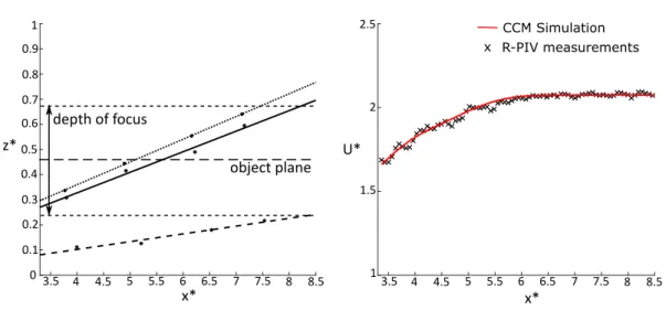
2.29 Left side is the laser sheet evolution in x∗ with the object plane (z∗OP) and the depth of focus shown. Right side is the velocity at y∗= 0.5 for the R-PIV measurement (black points) and the velocity obtained with the model for the same position (red line). . . 58
2.30 Error eq.2.19 is represented with Ure f∗ the velocity measured with R-PIV and Ucomp∗ the velocity predicted by the model. . . 58
3.1 Set-up for in-situ measurement of the velocity field in the water puddle. . . 61
3.2 Scheme of the experimental setup for stereoscopic measurements. . . 62
3.3 Scheme of the stereoscopic PIV principle with Sheimpflug settlement. . . 62
3.4 diameter of the image of a particle depending on its height in the puddle. . . 63
3.5 Images taken of particles. . . 64
3.6 Sketch of the shape of the diameter distribution of particles. . . 64
3.8 Intensity profiles obtained with the ray tracing model in the inhomogeneous configuration
(vertical sticks orange, brown and blue show locations of chosen profiles). . . 66
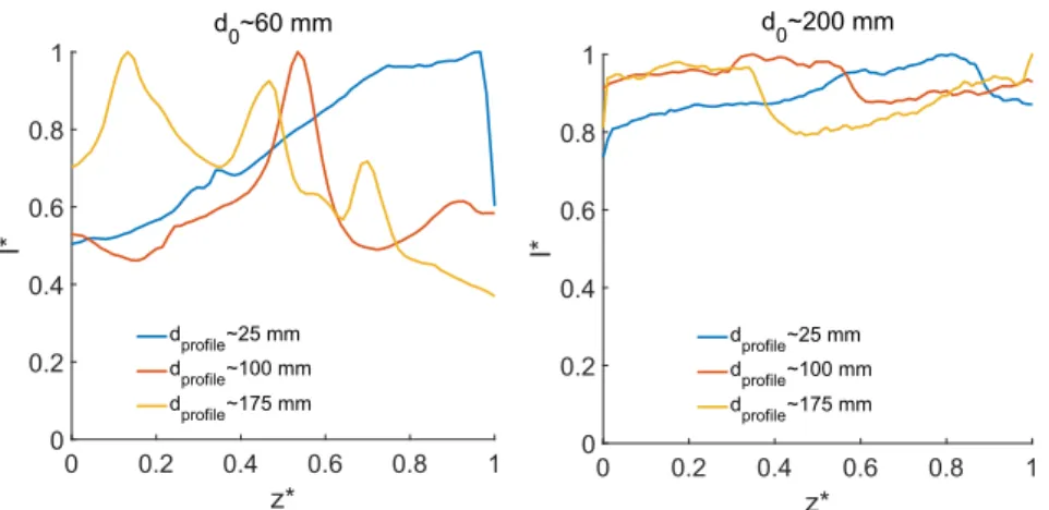
3.9 Intensity profiles obtained with the ray tracing model in the homogeneous configuration. 66 3.10 Intensity profiles obtained for two different distances, from the emerging laser point, at d0= 60 and 200 mm. . . 67
3.11 Scheme of the tire sculpture pattern for the PCY4. . . 69
3.12 Scheme of the tire sculpture pattern for the CCP. . . 70
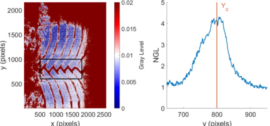
3.13 Maps of GL with the zone of calculation for GLcont. . . 71
3.14 On left : Gray level map with the averaging border zone in black. On right : mean Gray level profile in y. . . 71
3.15 On left : Gray level map with the averaging zone in black. On right : spatially averaged Gray level over y profile as a function of x. . . 72
3.16 On left : Gray level map with the averaging zone in black. On right : mean Gray level profile in y (y mean profile). . . 72
3.17 On left : Gray level map with the averaging zone in black. On right : Spatially averaged Gray level profile over y as a function of x. . . 73
3.18 R-PIV images of the contact patch area with the mask superimposed in red thin lines. . . 73
3.19 Description of the two flow zones (violet and brown lines) in front of the tire. . . 74
4.1 Contact patch of the tire for two successive measurements at V0= 50 km/h. . . 78
4.2 Fig.3.15 with a zoom in the contact patch area front edge (xc) with an uncertainty δ xc. . 79
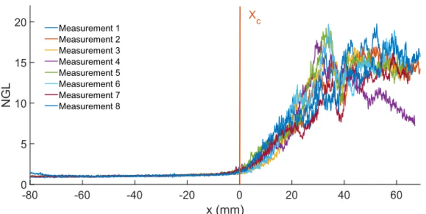
4.3 Evolution of the gray level in front of the central RIB for 8 measurements with a worn tire at v = 50 km/h. . . 80
4.4 Disturbances of the bubble column trajectory with the position of transverse small grooves. 80 4.5 Disturbances of the bubble column trajectory in PIV images. . . 81
4.6 Scheme of two different configurations of position of Type C grooves near the shoulder. . 82
4.7 Scheme of two different configurations of position of wear indicators in the grooves. . . 82
5.1 Scheme of the tire envelope with the fluid below and the corresponding velocity in the water bank. . . 85
5.2 Normalized falling velocity of particles of diameter dp= 35 µm over the time with both formulations. . . 88
5.3 Falling distance of a dp= 35 µm particle over the time (Right is a zoom on the early times). 89 5.4 Probability of presence in height of particles in the puddle. . . 90
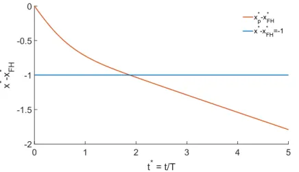
5.5 Scheme of the convected forehead of the water-bank. With xFH(t) = V0.t position of the forehead over the time . . . 90
5.6 Evolution of the velocity of the fluid at x∗(t∗) compared to the velocity of the solid particle. 92 5.7 Evolution of the relative position of a solid particle compared to the water bank forehead position. . . 93
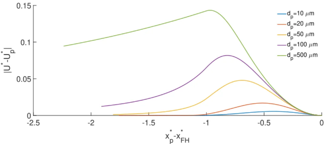
5.8 Top figure is the fluid velocity and the particle velocity at x = Xp∗(t∗). Bottom figure corresponds to the relative velocity U∗−Up∗. Both depend on the relative position of the particle compared to the forehead position. . . 93
5.9 Relative velocity U∗− U∗
p depending on the relative position of the particle for different
particle diameters. . . 94
5.10 Scheme of the boundary layer of interest. . . 94
5.11 Left are the normalized velocity profiles. Right is the growth of δBLover the time. . . 96
5.12 Sketch of the tire location and the fluid particle location at three different instants with the distance dist of traveling. . . 97
5.13 Left are the normalized velocity profiles for the blasius solution and the unsteady solution Equation.5.18. Right is the growth of δBLover the time. . . 97
5.14 Scheme of the transition zone where the two boundary layer shape should be joined. . . 97
5.15 Inputs profiles for the CCM in intensity, velocity and particle image diameter. . . 98
5.16 Velocity obtained depending on the boundary layer thickness δBL∗ = δBL hwater and the standard deviation for the Nim= 10000 snapshots averaged. . . 99
5.17 Velocity predicted by the model as a function of the boundary layer thickness δBL∗ = δBL hwater and the standard deviation. . . 99
5.18 Images of bubble columns with their size in the PCY4 tire grooves. . . 100
5.19 Problem considered for the tire groove flow analysis. . . 101
5.20 Scheme of the components of the electromagnetic field for a bubble. . . 102
5.21 Scattering section function of the bubble diameter. . . 103
5.22 Sketch of the problem studied. . . 103
5.23 Scheme of the bubble column. . . 104
5.24 Scheme of the bubble column with a particle above. . . 105
5.25 Transmission coefficient map as a function of bubble density and the bubble diameter with a bubble column thickness L = 1.5 mm. . . 105
5.26 Particle image diameter function of the height in the groove for both configurations. . . . 107
5.27 Spanwise velocity obtained with both CCM (left) and BCCM (right) models for the 2 reception optic configurations, z∗OP= 0 (top) and z∗OP= 1 (bottom). . . 108
5.28 Ensemble averaged spanwise velocity obtained with both CCM and BCCM models for the 2 reception optic configurations. . . 109
5.29 Spatially averaged velocity profiles obtained with the 4 configuration compared to the reference velocity field. . . 109
5.30 R-PIV image inside Type C grooves. . . 111
5.31 R-PIV image inside Type C grooves. . . 111
6.1 Instantaneous vector field measured for a new tire rolling at V0= 50 km/h through a puddle with hwater= 8 mm. . . 115
6.2 Ensemble averaged velocity component maps for new (top) and worn (bottom) tires. . . 116
6.3 RMS velocity component maps for for new (top) and worn (bottom) tires. . . 117
6.4 Spatially averaged velocity profiles in the WB UW B∗ in front of the tire. Red lines repre-sents the integration limits in x to obtain a global parameter < UW B>. . . 118
6.5 Spatially averaged velocity profiles at the shoulder Vs∗in front of the tire. . . 119
6.7 Ensemble averaged velocity component maps inside longitudinal grooves for both
con-figurations. . . 122
6.8 RMS velocity component maps for both configurations. . . 122
6.9 Ensemble averaged longitudinal velocity profiles along the tire grooves. (new tire) . . . . 122
6.10 Instantaneous and ensemble averaged longitudinal velocity profiles along the tire grooves. (new tire) . . . 123
6.11 Instantaneous and ensemble averaged longitudinal velocity profiles along the tire grooves (worn tire). . . 124
6.12 Velocity in the streamwise direction inside Type A and Type B tire grooves function of the wear indicator position in the image (worn tire). . . 125
6.13 Instantaneous and ensemble averaged transverse velocity profiles in the spanwise direc-tion inside Type A grooves. . . 126
6.14 Instantaneous and ensemble averaged transverse velocity profiles in the spanwise direc-tion inside Type B grooves. . . 127
6.15 Spatially and ensemble averaged velocity profiles obtained with both 2D2C and 2D3C configurations in the streamwise and spanwise directions. . . 127
6.16 Velocity map W inside longitudinal grooves. . . 128
6.17 Spatially and ensemble averaged velocity component W profiles inside A and B Type grooves (new tire). . . 128
6.18 A scheme of the tire grooves with their corresponding averaged transverse velocity com-ponent profiles for the new tire. . . 129
6.19 A scheme of the tire grooves with their corresponding averaged velocity profiles for the worn tire. . . 129
6.20 Instantaneous velocity maps V for new (left) and worn (right) tires. . . 130
6.21 Spatially averaged velocity in every Type C grooves in both cases. . . 131
6.22 Sketch of an example illustrating the position of Type C grooves in the contact patch area in percentage. . . 131
6.23 Velocity profiles in every the Type C grooves in both cases. . . 131
6.24 Ensemble averaged velocity component maps for CCP tire. . . 132
6.25 RMS velocity component maps for CCP tire. . . 133
6.26 Averaged longitudinal velocity profiles in the WB UW B∗ in front of the tire. . . 133
6.27 Averaged transverse velocity profiles at the shoulder Vs∗in front of the tire. . . 134
6.29 Sketch of the velocity components projected on the zigzag groove axis. . . 135
6.30 Velocity component U//and U⊥ profiles along the contact patch area. Orange lines rep-resents the weld positions. . . 135
6.28 Velocity map V∗= V /V0in the Type zigzag groove. . . 135
6.31 Velocity map V∗= V /V0in the Type W grooves. . . 136
6.32 Scheme of the projection of velocity vectors on the axes of the grooves with ~U//, the velocity in the groove direction and ~U⊥transverse velocity in the groove. . . 136
6.33 Mean velocity projected in the grooves a) in the groove axis and b) perpendicularly to the groove axis. . . 137
6.35 Averaged U//velocity component in a groove segment versus the location of its geometric
barycentre of the groove inside the contact patch area. . . 138
6.36 Inclination of the groove portions compared to the car rolling direction. . . 138
7.1 Spatially averaged velocity in the WB UW Bin front of the tire for different passes (left). Ensemble averaged < UW B> versus the vehicle speed (right). . . 142
7.2 Maximum velocity in the shoulder max.Vsin front of the tire for different passes (Left). Maximum velocity max.Vsand averaged velocity Vsfunction of the vehicle speed (Right). 143 7.3 Spatially averaged velocity in the WB UW Bin front of the tire for different passes (Left). Ensemble averaged < UW B> function of the vehicle speed (Right). . . 144
7.4 Maximum velocity in the shoulder max.Vsin front of the tire for different passes (Left). Maximum velocity max.Vsand averaged velocity Vsfunction of the vehicle speed (Right). 145 7.6 LW Bfor every measurements and its evolution function of the vehicle speed. . . 146
7.5 Measurement of the length of the water-bank for two single shot PIV measurements. . . 146
7.7 Normalized ensemble averaged velocity component maps for cases with V0∈ [30; 80] km/h.147 7.8 Isolines < U∗>= 0.4 of the normalised velocity component maps (from Fig.7.7) at each vehicle speed. . . 148
7.9 Normalised velocity component profiles in the water-bank and at the shoulder for V0∈ [30; 80] km/h. . . 148
7.10 Shape of the contact patch area with an increasing speed according to Todoroff et al. 2018 [72]. . . 149
7.11 Scheme of the hypothesis proposed for the loss of linearity in the velocity at high speed. 149 7.12 Velocity in the streamwise direction inside Type A grooves function of the vehicle speed. 150 7.13 Velocity in the streamwise direction inside Type B grooves for the worn tire function of the vehicle speed. . . 151
7.14 Ensemble averaged velocity profiles obtained at different vehicle speed. . . 152
7.15 Ensemble averaged velocity profiles obtained at different vehicle speed. . . 152
7.16 Velocity component map extracted from Fig.6.7 (up right) with the representation of the external and central part of both grooves. . . 153
7.17 Ensemble averaged velocity profiles in spanwise direction. . . 153
7.18 Lobes amplitudes as a function of the vehicle speed (left). Lobe amplitude definition with the case V0= 50 km/h (right) . . . 154
7.19 Sketch of the effect of Type D grooves linking longitudinal grooves with arrows high-lighting their expulsion direction. . . 154
7.20 Sketch of the differences in the boundary layer structure between Launay et al. 2017 [41] case and the tire rolling puddle flow case. . . 155
7.21 Visualisation of the bubble column creation zone in Type A grooves. . . 156
7.22 Sketch of the tire case with the vortex creation evolution between cross-section 1 and 5. . 157
7.23 Sketch of the squishing effect to create a second vortex in Type A grooves. . . 157
7.24 F∗with the corresponding deformation sketched in the contact patch area. . . 158
7.25 Visualisation of the link between Type B and Type C grooves. . . 159
B.2 Correlation map for a single interrogation window, right for raw images, left for treated
images. . . 177
B.3 Velocity maps for both raw images and preprocessed images. . . 177
B.4 Velocity profiles obtained for both raw images and preprocessed images. . . 177
C.1 Velocity maps for a decreasing interrogation window size. . . 179
C.2 Velocity profiles for a decreasing interrogation window size. . . 180
C.3 Velocity maps for a decreasing interrogation window size. . . 181
C.4 two velocity component, U//and U⊥ profiles for a decreasing interrogation window size. 181 D.1 Velocity component maps < V∗> for both object plane positions. . . 182
D.2 Transverse velocity component profiles < VA1∗ > for both object plane locations. . . 183
E.1 Hydraulic loop in laboratory for tire preliminary tests. . . 184
3.1 Number of statistical independent samples. . . 75
7.1 Table of the standard deviation in < UW B> normalised by the vehicle speed. . . 143
7.2 Table of the standard deviation in max.Vsnormalised by the vehicle speed. . . 144
7.3 Table of the standard deviation in Vsnormalised by vehicle speed. . . 144
7.4 Table of the standard deviation in UW Bas a percentage of the vehicle speed. . . 144 7.5 Table of the standard deviation in mean.Vsand max.Vsin percentage of the vehicle speed. 145
Tire Specific Vocabulary :
Shoulder Grooves RIBs RIBs Water Bank Contact patch Ground Tire envelope
1.1
Context and Motivations.
The tire is one element of a vehicle that is of first importance for adhesion of a vehicle on the ground it is rolling on and at a less important level for aerodynamic drag. It insures the contact with the road as an interface between a static domain, the road, and a dynamic object, the vehicle. At this interface the tire could be submitted to different conditions of adhesion, wet or dry, rough or smooth roads. This of primary importance for the car security and car performance. The global adhesion and the aerodynamic drags are functions of the car speed and the geometry design of the tire external shape.
The tire material and shape geometry constitution lead to different behaviours as a function of the previous parameters that pilot the global safety and drag of the vehicle. Fluid mechanics is a key point to improve the tire performances (safety, drag).
Concerning the influence on the aerodynamic drag force exerted on the vehicle, Croner et al. 2013 [22] showed that it is a function of the tire geometry for an isolated tire in a wind tunnel. Croner et al. 2013 [22] studied with both URANS (Unsteady Random Averaged Navier-Stokes) CFD (Computational Fluid Dynamics) simulations and experiments (Particle Image Velocimetry and hot wire) in a wind tunnel, the structure of the flow around an isolated wheel. This study allows to characterise the origin of vortical structures in the wake of the wheel as well as their unsteady behaviour. This improved the knowledge of the general structure of the air flow around a wheel without directly quantifying the effect on the total drag of a car/wheel system.
Different studies are focused on this aerodynamics drag from the system vehicle/tire studying the influence of the tires as Wang 2020 [76]. Wang conducted experimental PIV measurements on a system car/wheel in a wind tunnel. The general wake of the car can be influenced by many characteristics of the wheel as the tire pattern. The optimised pattern and the exact influence of the tire pattern on the drag was not quantified. However this study highlighted the direct influence of the tire design on the car total drag. The hydrodynamic behaviour of the tire at the interface with the road is another interest. By ensuring the grip of a tire on wet ground, the safety is improved. Many studies have been performed in order to analyse such a grip in presence of a wet ground as Beautru 2012 [9]. His study was focussed on the influence of thin water films between the road and the tire on the slippage of the car. The influence of the tire properties as well as the asphalt ones were investigated by quantifying the solid/solid contact between the tire and the road in order to determine the optimal conditions to ensure grip. They have done an experimental work based on DFT (Dynamic Frictional Tester) measurements in order to quantify the friction between the road and the rubber with small water height. This analysis highlighted the relation of
the friction coefficient as a function of the water height and the texture of the road. However, hydroplaning situation was not investigated.
In the present work, we aim to improve our knowledge concerning the aquaplaning phenomenon. This phenomenon is of a primary importance to ensure the grip properties on a wet road. The main requisite made to conceive a tire geometry is that the water has to be evacuated from below the tire when it is rolling on wet road (and a fortiori on a puddle). This has to be insured for maintaining a maximum tire shape/road contact area. For this the shape geometry contains grooves disposed to optimise the water evacuation whatever is the water presence. When a tire is rolling on a water puddle, whatever is this shape geometry, an high proportion of the incoming amount of water on the tire remains in front of it without evacuation. This imposes a pressure load in this zone that has to be minimised. Allbert 1968 [4], proposed in his paper a separation of the problem in three different zones as sketched on the figure 1.1 : the hydrodynamic zone, the viscodynamic zone and the dry zone.
Tire
TIRE
V
0
Hydrodynamic Viscodynamic DryFigure 1.1: Aquaplaning sketch of the 3 different zones.
The hydrodynamic zone is the zone where a strong pressure is developing in front of the tire when the amount of the drained water by the grooves or by the side of the tire is not sufficient. In their works (Horne and Dreher 1963 [32]) summarized the overall knowledge on the hydroplaning phenomenon in 1963. They discussed in this paper, the hydrodynamic pressure which increases proportionally to the square of the vehicle speed.
They shown that this hydrodynamic pressure lifts up the tire reducing the contact patch area between the tire and the road. This reduction of the contact patch area induces a reduction of the tire grip on the road. When the tire is totally lifted off and does not touch the road any more, the aquaplaning situation appears. More recently, they studied the speed limit to reach aquaplaning situation as a function of different parameters as the inflation pressure, tire footprint aspect ratio (see Horne and Dreher 1963 [32] and Horne et al. 1986 [33]).
The viscodynamic zone corresponds to a zone where the flow is mainly driven by the tire shape sculpture. This zone is limited to where the distance between the tire and the ground is of a few microns up to 0.1 mm. In this PhD work, the viscous effects in this micronic water zone between the rubber and the road are not addressed due to metroligical issues. Nevertheless in this zone the tire is submitted to a viscous slippage and not to the aquaplaning phenomenon. The preponderant physical effects in the water flow around the tire is here due to viscous forces more than pressure load. In the following study, this zone will be considered as the contact patch area, where the water flow is driven by the tire groove pattern.
zone inside the contact patch area, grooves have the objective to evacuate water. Small drops of water can remain between the tire and the road surface which influences the total grip of the tire. However, this zone will be considered in the whole study as the contact patch area and the effect of these drops is not addressed.
As a first point of view, the hydroplaning situation appears when the hydrodynamic pressure in the hydrodynamic zone is greater than the averaged load exerted on the tire by the total car in its aerodynamic movement. In order to minimise this situation and to produce tire with high performance on water, the amount of water drained by the tire should be maximised. The water is drained by two different mechanisms : 1) The amount of water driven off the tire path, by the side that is linked to the tire general contact patch area shape; and 2) the amount of water flowing in the tire grooves, drained through the contact patch area as a function of the tire sculptures. Thus, tread design has an impact on wet ground tire performances as during braking. Maycock 1965 [45] and Meades 1967 [46] showed the significant effect of the presence of tire tread compared to smooth tire on a wet ground. In his work, Maycock quantified the grip ability of a tire with the deceleration of the car during wet braking. A Braking force coefficient is calculated from this deceleration and is maximum when the grip is maximized because the deceleration during braking is directly linked to the grip of the tire. This allows them to highlight the importance of a patterned tire compared to smooth tire on different types of rough asphalt.
In terms of hydroplaning situation, the optimisation of tire pattern is subject to few studies as the numerical fluid/structure simulations (k-epsilon model for the fluid) made by Fwa et al. 2009 [26] where the hydrodynamic speed limit is studied as a function of different "non-realistic" tread design in order to quantify the influence of fully longitudinal, fully transverse or angled tread. This study demonstrated that a change of tread can lead to a change of hydroplaning critical speed up to 30 km/h. This study was made with smooth ground with different water film thicknesses from 1 mm up to 10 mm.
The tire design is of primary importance for the safety of the user and to increase the span life of the tires. Two main types of studies can be leaded in order to analyse the hydroplaning situation, numerical simulations and experimental works. Some studies are summarised in the following section.
1.2
Analysis of the flow in a puddle with a rolling tire.
In this section, we discuss the results and limitations of the different studies in the literature which at-tempted to quantify the hydroplaning process and to study the effect of the tire grooves geometries re-garding its wet ground performance.
Experimental observations were the first to allow the gathering of informations for a better under-standing of the hydroplaning phenomena. Further and mainly during this last decade numerical simula-tions, even not able to account for all flow scales or two phase flow phenomena, provide now a comple-mentary information to experimental one.
1.2.1 Experimental studies of the phenomenon.
The first attempt was qualitative estimation done using visualisations of the contact patch area using VLIF (Volume Laser Induced Fluorescence) as a contrast enhancement between the complete ground contact and the water around. Such technique was recently used to obtain quantitative results as function of car velocities (Todoroff et al. 2019 [72]).
1.2.1.1 Visualisation of the Contact patch area.
To perform these visualisations, fluorescent dye is placed in the water puddle. Images of the tire contact patch are taken with a high speed camera while a source of light illuminates the water puddle. This visualisation technique was first used by Yeager 1974 [81] and more recently by Todoroff et al. 2019 [72]. For both studies, the experimental measurements proposed take place on facilities where a glass plate covered with water is embedded into the road and allows the visualisations of the tire contact patch for true rolling conditions. The contact patch analysis is based on the contrast between the contact and the dyed water. The dye used to colour water is a fluorescein species. In Todoroff et al. 2019, images of the tire contact patch are recorded with a high speed camera. Thus the analysis of the contact patch area evolution with a growing vehicle speed V0can be performed. Usually, Todoroff used a water height 1 mm for both worn and new tire configurations. The vehicle speeds used range from V0= 8 km/h to V0= 90 km/h.
From this last study we can see instantaneous images on the figure 1.2. This was recorded on the Michelin’s test facility with a summer tire at V0= 50 km/h. More details on the test facility are given in the chapter 3. The main problem is a correct detection of the contact patch area. This necessitates the use of digital image treatment tools to first increase the signal to noise ratio and secondly to have automatic criteria to treat the different samples obtained for a same case and to be able to do the best geo-metrical coincidence as possible for each sample in order to perform ensemble averaged of the measured quantities.
From the recorded images a Michelin’s in-house treatment algorithm improves the contrast between the dry zone (black part from RIBs/road contact) and the water zone (green fluorescence from dyed water). This clearly allows to determine the boundary of the contact patch area of the tire. In so the study was able to furnish the evolution of the contact patch area as a function of the vehicle speed V0. In the work by Todoroff et al. 2019 [72] this is done for a summer tire but it can also be done for different tire sculptures. From this kind of observations it is supposed that the contact patch area have to be maintained the most important as possible compare to the initial null velocity of the vehicle. In so this kind of study is of first importance to furnish a global parameter to characterise a tire shape.
1.2.1.2 Velocity measurements in presence of water
The literature velocity measurements of the water flow around and below a rolling tire through a puddle is very sparse.To our knowledge, quantitative measurements have only been performed by Suzuki and Fujikama 2001 [69]. In this work, the experimental method proposed is based on a facility where a glass plate covered with water is embedded into the road and allows the visualisations of the tire contact patch area for true rolling conditions, as used by Todoroff for visualisations. Solid particles of Millet (of diameter 1 to 1.5 mm) seeded the water as tracers and some images were recorded with an high speed camera at 1500 Hz and illuminated by 4, 500 W, continuous light sources. With long exposure time images, the particles appeared as strikes on the images. From the length of these strikes, the displacement of the particles during the exposure time was calculated. Thus, the velocity can be deduced from these displacements.
This method allowed the authors to determine the velocity field in front of the tire on a grid whose random location of vector origin is inherent to the technique. The influence of the angle of the grooves on a cornering effect of the tire was discussed. This technique allowed the authors to produce very interesting experimental information about the velocity in front of the tire. However, the velocity inside the tire grooves was not addressed with this technique and the velocity vectors density obtained in front of the tire remained low and could be improved.
1.2.2 Some Numerical studies of the hydroplaning phenomenon.
The use of numerical simulation to analyse the flow induced during an hydroplaning phenomenon is largely more difficult to obtain as explained before and very rare work are existing on the subject with such tool. Nevertheless, the recent improvements of computational power allows now to envisage such hydroplaning simulation even more taking into account for fluid/structure deformations. Main part of the numerical simulation use an Eulerian point of view.
The tire deformation is simulated by Finite Element method (FE) in every work described in the following. For the fluid, different methods can be used as Finite Difference (FD), Finite Element (FE) and Finite Volumes (FV). For FD method, two main works can be found in the literature with the same characteristics for the simulations. Oh et al. 2008 [59] and Kim and Jeong 2010 [36] present simulation results for a tire rolling using single phase RANS (Random Averaged Navier Stokes) simulations. Oh et al. 2006 [59] showed in their simulations the effect of the increase of the vehicle rolling speed (from 0 km/h to 90 km/h) on the hydrodynamic pressure load on the tire. The water height in this study is set to different heights from 5mm to 20 mm with a straight-grooved tire on a smooth ground. In Kim and Jeong 2010 [36], the same simulations are performed but with an increase of the fluid-structure coupling performance allowing the analysis of a patterned tire. This highlighted the importance of a fully patterned tire on wet grounds. The hydrodynamic pressure exerted on the tire is lower for a patterned tire than for a smooth tire.
For FE method, one work is by Koishi et al. 2001 [38] where simulations of hydroplaning situations are performed for 10 mm water height with a patterned tire (V-shaped grooves) on smooth ground. This study allows to highlight the difference in the hydroplaning critical speed (vehicle speed needed to lose all contact between the tire and the road) between a V-shaped tire mounted in the good way and reversely. The hydroplaning critical speed is quantified as the speed for which the contact force between the tire and
the road becomes null.
Few works can be cited using the FV method for the fluid as the one by Cho et al. 2006 [18], where RANS simulations are performed for an inviscid fluid and a 10 mm water height puddle with a fully straight-grooved tire and a patterned tire on smooth ground. These simulations shows differences on the hydrodynamic load exerted on the tire for both tire model with vehicle speed from 40 km/h to 80 km/h. In Vincent et al. 2011 [75], LES simulations are performed with a 8 mm water height. In this study, the hydrodynamic load on the tire is presented together with the contact patch area for three different tire models with a fixed speed at 50 km/h. One is smooth, and the two others are patterned on smooth ground. This shows the importance of the pattern of the tire with a drastically decreased load with patterned tires. Finally, Kumar et al. 2012 [40] also performed simulations for smooth tire on smooth ground in a 10 mm water height puddle. Various inflation pressures were tested showing that the hydroplaning speed is increased with the increase of the inflation pressure.
All these simulations have been significant advances in the understanding of hydroplaning. They also highlight limitations of the simulation in such complex issues. Particularly, except for Vincent et al. 2011 [75] study, all the numerical studies of hydroplaning phenomenon do not deal with the multiphase aspect of the flow even if it can have an influence on the flow inside the tire grooves. These studies also show difficulties to determine the flow inside fully patterned tire grooves because of the computational time cost if a sufficient refined meshing inside the groove is accounted. Therefore, simplified geometries are often used.
This is one of the reasons why the importance of tire pattern compared to smooth tire is highlighted by these studies, but the differences between two patterned tires is difficult to determine.
Finally, simulations are always proposed for high water height which are not realistic conditions. In real road situations, the range of such height is about 1 mm during heavy raining events (see Hermange 2017 [30] page 26).
A different approach has been recently proposed by Hermange 2017 [30] with a Smoothed Particles Hydrodynamics (SPH) Lagrangian method for the fluid displacement. Simulations were here performed for a vehicle speed of 80 km/h with a water height of 1 mm. This method shows advantages for free surface flows and in term of computational cost as refinement could be compensated by selecting pref-erential zones for which more particles are accounted. This method also allows to perform calculations with rough grounds which are more similar to the real asphalt. However some difficulties still exists as soon as turbulence or multiphase flow have to be accounted.
Numerical simulations have been extensively used to gather informations on the hydroplaning phe-nomenon. Nevertheless, detailed quantitative descriptions of real flow situation were never addressed particularly in the tire grooves.
1.2.3 Purpose of this work.
Facing all the interrogations and missing informations as pointed out from the previous review a main pur-pose of the present PhD work is to provide an experimental method based on Particle Image Velocimetry (PIV) which allows In-Situ measurements of the water flow in the puddle with a real car rolling through it.
If this objective is respected more precision and information will be given for water flow in front of the tire, in some tire grooves. One objective is also to obtain the better as possible repeatability, precision
and a vector density high enough to describe in details the flow structure.
Before focusing on the description and characterisation of the new PIV extension that is developed in this work to fulfil the objective (Chapter2), let’s summarize the knowledge of the flow structure that we just deduce from the previous literature review.
1.3
The flow structure.
1.3.1 Different zones of the flow.
We have previously indicated that it is difficult to measure the fluid flow in the viscous zone due to dimension of the thin film (Fig.1.1). In this work the flow analysis is focused on the two other zones described in Section.1. The first one is the hydrodynamic zone in front of the tire. In this work we split this specific zone with the one of the flow in front of the tire (water-bank zone) and an other one on the sides, the shoulder zone. In the first subpart, a certain amount of water is driven off the tire path at the shoulder zone (by a mean symmetry 2 parts) and a certain amount is accumulated in front of the tire. The second is the dry contact zone. In this zone, the ribs are supposed to be the part constituting the adhesion (along the constant rolling) with the ground. In the grooves, the water is stored and drained by the tire groove flow. Specific flow behaviours are present for every subparts (in the water-bank, at the shoulder and inside the grooves) of the flow and will be discussed here.
1.3.2 Flow in front of the tire.
In front of the tire (in the water-bank), the structure of the flow can be decomposed in three parts. (i) far from the tire a free-surface flow appears. (ii) the flow is subject to an acceleration phase with an increase of the water height. (iii) when we get closer to the tire, the flow becomes confined between the tire envelope and the ground (Fig.1.3). Based on literature and especially Hermange 2019 private communication [31] simulations, it appears (Fig.1.3) that the velocity of the fluid in the first part (i) is null (in the figure the velocity is normalised by the vehicle speed).
Tire envelope Ground Fluid Viscodynamic zone (i) (ii) (iii) UWB
Figure 1.3: Scheme of the geometry of the flow in the Hydrodynamic zone (with the three parts high-lighted) with the corresponding averaged velocity profile over the water height in z.
in this zone could be associated to a flow at velocity UW B∗ in a divergent channel in the ground referential with a flow coming from the contact patch area in the x direction.
In the referential of the tire, the flow arrives on the tire. This can be associated to a water flow past an obstacle. From a schematic point of view, it can be considered as an obstacle with a rectangle shape. The free-surface flow passing a rectangular or cubic obstacle is extensively studied in the literature. Thus a part of the water arriving on the tire will be driven off the tire path by the side at the shoulder of the tire. Nevertheless it is clear here that free surface can add complexities as the formation of a hydraulic jump surrounding the obstacle and the formation of a horseshoe vortex. Mignot and Rivière 2010 [52], showed with visualisations that two flow regimes can be distinguished for this last case. For high Reynolds number, the "breaking type" of flow appears with a length of the hydraulic jump greater than the length of the horseshoe vortex. For low Reynolds numbers, the "separation type" of flow appears with a greater length for the horseshoe vortex than the hydraulic jump. The critical Reynolds number between both types depends on the Froude number and the ratio water height/obstacle width. They also showed that three parameters can influence the length of the hydraulic jump and the horseshoe vortex, the Reynolds number, the Froude number and the ratio water height/obstacle width. The horseshoe vortex presence can be interesting knowing the presence of vortices in the tire grooves. The conditions of creation of these grooves depend on the separation of the boundary layer on the ground near the obstacle. This was especially observed by Launay 2017 [41].
In some specific conditions of low water height/obstacle width ratio, the bow-like wave in front of the tire becomes a wall-jet-like bow-wave. This jet height depends on the Froude number and the water height/obstacle width ratio as observed with visualisations by Rivière et al. 2017 [63]. For the rolling tire conditions, the water height/obstacle width ratio is approximately 0.04 which is lower than 1 for a whole tire. Therefore, the creation of a wall-jet-like bow-wave in the tire vicinity at the free surface can be assumed as sketched Fig.1.4. According to Equation 9 in Rivière et al. 2017 [63], the dimensionless jet height normalised by the kinetic height h∗jet= hjet/(U2/2g) = 4 (where U is the fluid velocity in the obstacle referential and g is the gravity acceleration) with tire conditions. The maximum value encountered by the authors is h∗jet = 1.4. Therefore, the tire flow conditions are extreme and can slightly diverge from the results of the literature.
Tire envelope Ground Fluid
wall-jet
Figure 1.4: Sketch of the wall-jet in front of the tire.
1.3.3 Flow in tire groove.
Two different levels of description are interesting inside the tire grooves. A primary flow is considered as the flow in the longitudinal groove direction whatever the groove axis is in the longitudinal car direction or in the transverse car direction. This primary flow corresponds to the amount of water driven through the contact patch area by the grooves and evacuated down the tire or on the sides of the dry zone. A
1 bubble column 2 bubble columns
Figure 1.5: Zoom on tire grooves from Todoroff et al. 2019 [72].
secondary flow is detailed in this work considering transverse vortex structures of the flow all along the longitudinal tire groove direction.
The velocity of the tire envelope in the ground referential in the contact patch area with no slip condition is Ve= 0 . Thus the wall displacement velocity of the channel formed by the groove is quasi-null in the ground referential. If we consider the channel flow with a fluid velocity U = 0.1.V0in the ground referential (see Chapter6, Fig6.10) with the following definition for the Reynolds number Re =U.DH
ν (where DH is the hydraulic diameter and ν is the kinematic viscosity of the water), for a car rolling at V0= 50 km/h, the Reynolds number is about Re = 3000.
This Reynolds number is high enough to consider a potential presence of turbulence. However in this highly unsteady phenomenon with a short contact patch area length (90 mm approximately for V0= 50 km/h for a new tire configuration according to Todoroff et al 2019 [72]), the flow regime can not be established and the real presence of turbulence remains to be discussed.
The second interesting feature of the flow is its 3D structure inside the grooves. If we now get back on Todoroff et al. 2019 [72] visualisations and take a closer look inside the tire grooves (Fig.1.2), there are rich information on the flow structure inside the tire grooves. For example we can observe the existence of multiphase flow with straight bubble columns inside the tire grooves. This observation in longitudinal grooves can be observed also for an other tire on the figure 1.5.
From this last image the bigger grooves contain 2 bubble columns whereas there is only one bubble column in the smaller grooves. Note that these grooves have respectively an aspect ratio of 2 and 1. These bubble columns seems generally straight inside the tire grooves. An apparent concentration of bubble lets think that they participate to a structure that could be due to some flow vortices in the grooves. Multiple forces are involved in a bubble displacement inside a rotating flow as the drag and lift forces which are subject to many research (see Rastello et al. 2009[62] and Rastello et al. 2011[61]). Considering centrifugal forces, bubbles, lighter than the water, will converge to the core of the vortices after some time (as demonstrated with experimental visualisations by Chahine 1995[16] in Figure 18.6.1). This convergence was also discussed by Caridi et al. 2017 [15]. In their paper, they discussed the influence on the particles distribution of heavier or lighter particles in vortices. This was made in order to quantify the good density ratio between their particles and the air flow studied to obtain homogeneous partition
Figure 1.6: Sketch of the vortices inside the tire grooves from Yeager 1974 [81].
of particles for PIV. They showed that when the particles are way lighter than the fluid, the particles will converge to the core and the density of particles outside the vortex core will be too low to perform PIV measurements. In our case, air bubbles are 1000 times lighter than the water. Therefore, bubbles will converge to the core of the vortices.
While the visualisations shown in this reference clearly identify the presence of elongated filaments probably related to local two-phase flow (bubble column or bubble cluster), the author do not highlight especially this feature of the flow. On the other hand, Yeager implicitly relates these filaments to hypo-thetical longitudinal vortices like those depicted in Fig.1.6
More recently these vortices inside the flow tire grooves are observed but with only an air flow sur-rounding the tire for an aerodynamics study by Croner 2014 [21] and for which the creation mechanism may be similar. Croner’s PhD is focused on the analysis on the air flow surrounding a tire based on numerical simulations and experimental measurements presented in Croner et al. 2013 [22] (already presented in Section.1.1). The vortices inside tire grooves were mentioned in the numerical simulation results without focusing on it. The main purpose of her PhD. being the analysis of the wake for drag reduction.
Nevertheless, the vortex presence in the groove and with a water flow due to tire rolling on a water puddle for example, was neither quantitatively measured nor simulated before the present work. It is thus one challenge for this work to be able to prove their existence. This will be presented in the Chapter 5 and further with quantitative original PIV measurements.
As a first approach, before measuring quantitatively these vortices, the analysis of the visualisations from Todoroff et al. 2019 [72] allows us to determine differences of the flow structure from worn to new tire configurations. In the summer tire grooves we can observe the number of bubble columns to determine the number of vortices per grooves. The largest tire grooves have an aspect ratio (width/height) of 2 and the smallest grooves at the shoulder have an aspect ratio of 1. For the worn tire case, the corresponding value of the aspect ratio is respectively 6 and 3. Thus the number of vortices can be analysed in both cases Fig.1.7.
New Tire Worn Tire 4 Column s 2 Column s 2 Column s 1 Column
Figure 1.7: Groove images for both new and worn tires. Upper image is the smallest groove and lower image is the largest groove (from Todoroff et al. 2019 [72])
We can observe here a difference in the number of bubble columns that are visible in both cases. This number seems to depend on the aspect ratio of the tire grooves. This hypothesis is accounting and have to be ascertained by the present measurements which are performed inside the tire grooves (6).
1.3.4 Conclusion.
A first idea of the flow structure allows us to identify a priori the general behaviour in the different parts of the flow. In front of the tire, the tire constitutes an obstacle and thus a part of the flow will be driven off the tire path at the shoulders. An other part of the flow, in front of the central RIBs of the tire, is pushed forward by the tire and is not a free-surface flow but more a channelled flow between the ground and the tire. Inside the tire grooves, the flow seems to be a high Reynolds number flow with a too short distance to establish in a net regime. The secondary flow constituted by the vortices depends on the configuration of the longitudinal groove and its aspect ratio.
1.4
Thesis organisation.
As we have seen at the best of our knowledge there is no existing quantitative velocity field measurements in the different zones described above. The purpose of this work is first to develop an experimental method based on PIV before adapting this method to the tire measurements. Therefore the Chapter 2 introduces, the experimental method developed here and called R-PIV and that is an extension of the more classic Planar PIV. It is described and validated with a laboratory channel flow study. In this chapter, the specific optical properties of the method will be discussed with their effects on the PIV field calculations. This will lead us to revisit the PIV optical models for classic PIV as we adapt them to particular illumination technique. An experimental validation is proposed from the test bench results as analytic solutions are known and classic PIV measurements are further done.
In the Chapter 3, the adaptation of the set-up to IN SITU tire measurements is described with the optical properties associated to the tire measurements. The tire models tested are also described with the digital image processes necessary to use to coincide the coordinate system as soon as a fixed tire case
study needs several measurement repetition to ensure a statistical convergence. Then description of the image processing and velocity field calculations are described with the flow zone studied in the tire case. The Chapter 4 is dedicated to the analysis of the different sources of variability for the application of the R-PIV to the IN SITU tire flow. In this chapter, the main different sources of bias are discussed, from the control parameter associated to the set-up to the hydrodynamic and metrological variations from a measurement to an other.
The Chapter 5 is dedicated to a metrological discussion. In this chapter, a discussion about the tracer ability is conducted to precise the uncertainty associated to the particles used for seeding the flow. In a second part, a discussion on the effect of a probable boundary layer on the R-PIV measurements in front of the tire is proposed. Finally the complex case of the effect of the multiphase flow (inclusion of micro bubbles inside the vortex cores) on R-PIV measurements is discussed in order to show what part (in height) of the velocity field is described in this zone.
Finally, a presentation of the results in every parts of the flow is shown in Chapter 6 with a discussion, on the hypothesis proposed and on the origin of the different phenomenons that are described, in the Chapter 7.
2.1
The Particle Image Velocimetry (PIV).
2.1.1 planar PIV technique.
The particle image velocimetry (PIV) is a well known technique used in fluid mechanics to measure velocity fields in fluid flows. In PIV, particles are seeding the fluid flow of interest and are illuminated by a double pulsed laser light sheet. Images of these particles are recorded on a camera at two successive instants, t and t + dt, and the velocity field is calculated from correlation techniques, as cross-correlation, between two successive images.
2.1.1.1 Description of a planar PIV set-up.
For planar PIV measurements (denoted as P-PIV, in the following), the working distance is usually of a macroscopic scale. The working distance could range typically between 50 mm to 1000 mm. With these conditions, the depth of focus of the camera, which is proportional to the working distance, is large compared to the light sheet thickness (at least few millimeters). Therefore, the depth over which particles contribute to the cross-correlation is driven by the thickness of the laser sheet illuminating the particles.
For P-PIV measurements in a channel flow, the laser sheet should be as thin as possible and ideally perfectly parallel to the camera recording plane to avoid distortion of the images (Fig.2.1). A constraint to use this technique is that the laser sheet should be, most of the time, perpendicular to the camera axis. This could be difficult to respect in particular cases where the flow does not possess two optical accesses.
outlet Inlet
Laser head
Camera
Laser P
Figure 2.1: Scheme of a light sheet illuminating particles for P-PIV measurements.
delay dt and two images are recorded. The displacement of particles between both images (dx,dy) can be calculated using a cross-correlation algorithm. Therefore the velocity field is determined with (U =dxdt, V =dydt).
2.1.1.2 Description of the cross correlation.
After recording, images are matrices of pixel whose grey levels describe the intensity re emitted from the field of view. The cross-correlation is applied to small areas of the images called interrogation windows with a size (δ wx, δ wy) in pixels ((∆wx, ∆wy) in mm) depending on the displacement of particles. These windows must be small enough to consider that all the particles in the window have the same velocity. The cross-correlation algorithm consists in finding the pattern produced by the particles in image one interrogation window at time t, in the second image at time t + dt (Fig.2.2) (Adrian and Yao 1985 [3] and Adrian 1991 [2]). Image 1 Image 2 z U dt x x dxx dx dt V = Particles in Image 1 out Image 2
Particles out Image 1 in Image 2
Figure 2.2: Scheme of the two images recorded with the interrogation windows represented.
If I1(X ,Y ) is the intensity pattern in the interrogation window centred in (X ,Y ) in image 1 and I2(X + δ x,Y + δ y) the intensity pattern of a window centered in (X + δ x,Y + δ y) in image 2, the cross-correlation between I1and I2is calculated according to Scarano and Riethmuller 2000 [64] :
R12(δ x, δ y) =
Z X+∆wX/2
X−∆wX/2
Z Y+∆wY/2
Y−∆wY/2
I1(X + x,Y + y) · I2(X + x + δ x,Y + y + δ y)dxdy (2.1)
In this work, the cross-correlation is calculated with a commercial Software (Davis from Lavision). With a discrete intensity distribution in pixels on the camera sensors, the discrete cross-correlation func-tion is calculated as expressed by Willert and Gharib 1991 [79] :
R12(δ x, δ y) = δ wx
∑
i=−δ wx δ wy∑
j=−δ wy I1(i, j) · I2(i + δ xpx, j + δ ypx) (2.2)where δ xpxand δ ypxare the displacement components between image 1 and 2 in pixels for an interroga-tion window centered in (0, 0) in image 1.
To determine the particle displacement in such an interrogation window, the displacement (δ xpx, δ ypx) maximising the cross-correlation function is found. According to Kean and Adrian 1992 [34], the cross-correlation function can be decomposed into 3 parts. RC is between backgrounds of image 1 and image 2. RF takes into account the correlation of image of particles in image 1 with image of particles that are different from them in image 2. RD is the displacement component which corresponds to the correlation of particles in the image 1 with their own images on image 2. These components are sketched in Fig.2.3 : I1 I2 P1 P1 P2 P2 dt 3 correlation components R :C R :F R :D P1 P2 x P1 P2 x P1 P2 x x x P1 P2 x P1 P2 x P1 P2 x
Figure 2.3: Scheme of the decomposition of the cross-correlation function.
This leads to a cross-correlation function between image 1 and 2 that is the sum of these 3 components ( Adrian 1988 [1]) :
R12= RC12+ RF 12+ RD12 (2.3)
An exemple of the cross-correlation and its components is displayed in Fig.2.4 :
0 50 0.5 R12 C 50 y x 1 0 0 0 50 0.5 R12 F 50 y x 1 0 0 0 50 0.5 R 12 D 50 y x 1 0 0 0 50 0.5 R12 50 y x 1 0 0
![Figure 1.6: Sketch of the vortices inside the tire grooves from Yeager 1974 [81].](https://thumb-eu.123doks.com/thumbv2/123doknet/14717397.750456/31.892.277.615.119.404/figure-sketch-vortices-inside-tire-grooves-yeager.webp)