Assessment of finite element approximations for nonlinear flexible multibody dynamics

(1)

ASSESSMENT OF

FINITE ELEMENT APPROXIMATIONS

FOR NONLINEAR FLEXIBLE

MULTIBODY DYNAMICS

by

DAVID THOMAS ROBERTS

B.A.E.M., University of Minnesota (1985)

SUBMITTED TO THE DEPARTMENT OF AERONAUTICS AND ASTRONAUTICS

IN PARTIAL FULFILLMENT OF THE REQUIREMENTS

FOR THE DEGREE OF

MASTER OF SCIENCE at the

MASSACHUSETTS INSTITUTE OF TECHNOLOGY

May 1991

The author hereby grants to MIT permission to reproduce and to distribute copies of this thesis document in whole or in part.

Signature of Author

Department of Aeronautics and Astronautics May 10, 1991

Certified by

_{Certified by}

,

_{David S. Kang}

W

Technical Staff, C.S. Draper Laboratory Thesis Supervisor

Approved be

Approved by John DI'gundji

Professor, Department of Aeronautics and Astronautics . A Thesis Supervisor

Accepted by _,4,

PrUessor Harold Y. Wachman

Departmental Graduate Committee

(2)

ASSESSMENT OF FINITE ELEMENT APPROXIMATIONS FOR NONLINEAR FLEXIBLE MULTIBODY DYNAMICS

by

DAVID THOMAS ROBERTS

Submitted to the Department of Aeronautics and Astronautics on May 10, 1991

in partial fulfillment of the requirements for the degree of Master of Science in Aeronautics and Astronautics

ABSTRACT

Systematic investigation is made of effects of kinematic assumptions and finite element approximations in the context of nonlinear flexible multibody dynamics. Two nonlinear beam finite elements are consistently derived from virtual work principle using Bernoulli-Euler and Timoshenko beam kinematics. Initial assessment is made by studying convergence properties of element formulations with eigenvalue problems: free vibration, static buckling, and dynamic buckling. Equations of motion are derived for rigid central body with flexible appendage using virtual work principle. Virtual work principle allows natural and consistent discretization of flexible appendage using finite element method. Nonlinearities in flexibility are explored through dynamics examples using beam finite elements. Application of dynamics formulation is made to a realistic scenario involving space shuttle remote manipulator arm with attached payload. Contribution of nonlinear theory, in both formulation and solution, is assessed.

Thesis Supervisor: David S. Kang, Ph.D.

(3)

Acknowledgements

I would like to express my sincere gratitude to my thesis supervisor, David S. Kang, who made substantial contributions to every aspect of my education, and graciously gave his time and energy on my behalf.

I would like to acknowledge the support and friendship of my Draper Laboratory colleagues: Joe Nadeau, Van Luu, Howard Clark,

Mark Henault, Dave Dellagrotte, and Ashok Patel.

Last, but not least, I would like to express my heartfelt appreciation to my family, for all the love and encouragement they have so freely given.

(4)

This thesis was supported by The Charles Stark Draper Laboratory, Inc., under Internal Research & Development 332.

Publication of this thesis does not constitute approval by The Charles Stark Draper Laboratory, Inc. of the findings or conclusions contained herein. It is published for the exchange and stimulation of ideas.

I hereby assign my copyright of this thesis to The Charles Stark Draper Laboratory, Inc., Cambridge, Massachusetts.

David T. Roberts, CAPT, USAF

Permission is hereby granted by The Charles Stark Draper Laboratory, Inc. to the Massachusetts Institute of Technology to reproduce any or all of this thesis.

(5)

Table of Contents

C.1

C.2

C.3

B: Time Integration Schemes...142

Newmark Integration for Linear Systems ... 143

Incremental Form of Newmark Integration ... 144

Error Sources in Newmark Integration...147

Fourth-Order Runge Kutta Integration... 148

Implementation with Equations of Motion ... 150

C: Convergence Data... ... 153

Free Vibration...153

Static Buckling... 159

Dynamic Buckling ... 162

Appendix D: RMS Finite Element Model...163

Appendix E: Solution of Timoshenko Frequency Equation...165

(8)

List of Fihures

List of Figures

Figure Figure Figure 2.1. 2.2. 2.3. Figure 2.4. Figure Figure Figure Figure 3.1. 3.2. 3.3. 3.4. Figure 4.1. Figure 4.2. Figure 4.3. Figure 4.4.

Figure 4.5.

Figure 4.6. Figure 4.7. Figure 4.8. Figure 4.9. Figure 4.10. Figure 4.11.

Rigid body with flexible appendage... 23

Lumped mass discretization of the flexible appendage...32

Lumped mass/inertia discretization of flexible appendage ... 37

Relative displacement of ith nodal body...38

3-D beam coordinate system... 47

Kinematics of Bernoulli-Euler beam theory...48

Kinematics of Timoshenko beam theory ... 48

Local coordinates for 2 node beam element. ... 52

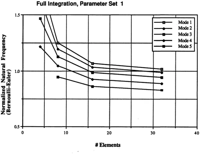
Convergence for CO beam, consistent mass, full integration, parameter set 1... 78

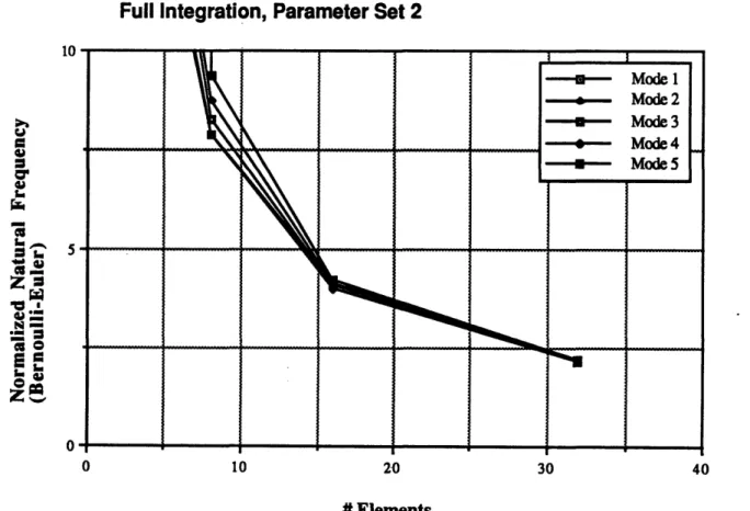
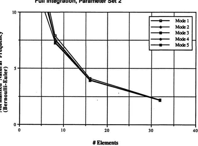
Convergence for CO beam, consistent mass, full integration, parameter set 2 ... 79

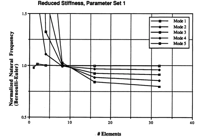
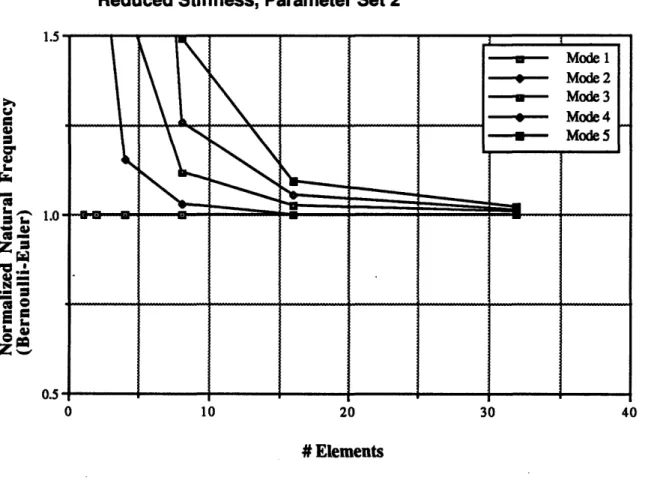
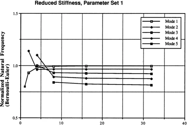
Convergence for CO beam, consistent mass, reduced stiffness, parameter set 1 ... 80

Convergence for CO beam, consistent mass, reduced stiffness, parameter set 2 ... 81

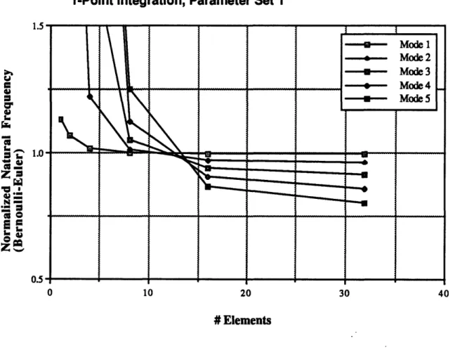
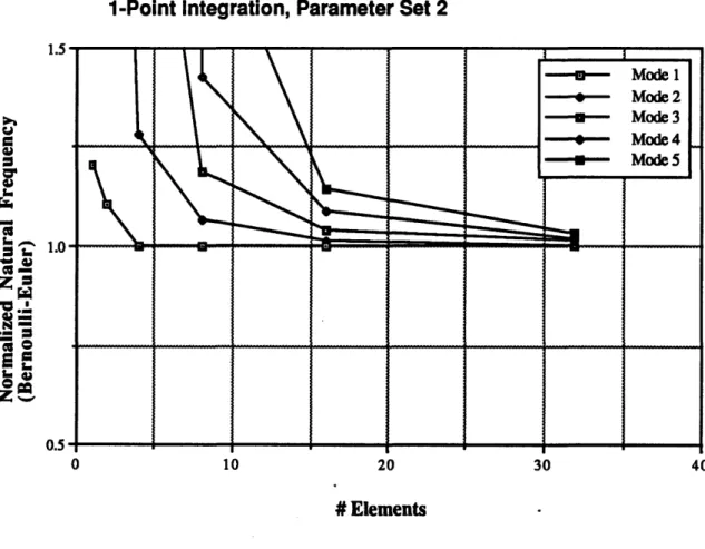
Convergence for CO beam, consistent mass, uniform 1-point integration, parameter set 1...82

Convergence for CO beam, consistent mass, uniform 1-point integration, parameter set 2... 83

Convergence for CO beam, lumped mass, full integration, parameter set 1...84

Convergence for CO beam, lumped mass, full integration, parameter set 2 ... 85

Convergence for CO beam, lumped mass, reduced stiffness, parameter set 1 ... 86

Convergence for CO beam, lumped mass, reduced stiffness, parameter set 2 ... 87

Convergence for C1 _{beam (Rayleigh), consistent mass,} full integration, parameter set 1... 88

(9)

List of Firures Figure 4.12. Figure 4.13. Figure Figure 4.14. 4.15. Figure 4.16. Figure 4.17. Figure 4.18. Figure 4.19. Figure 4.20. Figure Figure Figure 4.21. 4.22. 4.23.

Convergence for C1 _{beam (B.E.), consistent mass, full}

integration, parameter set 1... 89

Convergence for C1 beam, consistent mass, full integration, parameter set 2 ... 90

Exact vibration mode shapes, Bernoulli-Euler theory...92

Convergence for CO beam, full integration of stiffness, parameter set 1...95

Convergence for CO beam, full integration of stiffness, parameter set 2...96

Convergence for CO beam, reduced integration of stiffness, parameter set 1 ... 97

Convergence for CO beam, reduced integration of stiffness, parameter set 2 ... 98

Convergence for C1 _{beam, full integration of stiffness,} parameter set 1 ... 99

Convergence for Cl beam, full integration of stiffness, parameter set 2... ... 100

Cantilevered beam under distributed axial load...101

Natural frequencies for Po < Per, parameter set 1...103

Convergence for dynamic buckling, parameter set 1...104

Figure 5.1. Figure 5.2. Figure 5.3. Figure 5.4. Figure 5.5. Figure 5.6. Figure 5.7. Figure 5.8. Figure 5.9. Flow diagram for dynamic simulations...10

Spin-up of cantilever beam...111

Hub motion prescribed by equation (5.2.1) ... 1...12

Schematic of finite element model, analogous to figure 2.1 ... 113

Axial displacement of beam tip for case 1, 2 elements... 116

Transverse displacement of beam tip for case 1, 2 elements. ... ... 116

Transverse displacement of beam tip for case 1, 4 elem ents. ... 117

Figure 5.10. Transverse displacement of beam tip for case 1, 8 elem ents ... 118

(10)

List of Figures Figure 5.11. Figure 5.12. Figure Figure 5.13. 5.14. Figure 5.15. Figure 5.16. Figure 5.17. Figure 5.18. Figure Figure 5.19. 5.20. Figure 5.21. Figure 5.22. Figure 5.23. Figure 5.24. Figure 5.25.

Axial displacement of beam tip for case 1, 16

elements. ... ... 119

Transverse displacement of beam tip for case 1, 16

elements... ... 119

Axial displacement of beam tip for case 2, 8 elements...121 Axial displacement of beam tip for case 2, 16

elements. ... ... 121

Transverse displacement of beam tip for case 3, 2

elements... ... 122

elements. ... ... 123

elements...124 Torque time history applied to orbiter...126 Finite element model of remote manipulator arm in

straight out position...127 Orbiter response to pulse torque, assuming rigid and

flexible ... ... 128

Orbiter response to pulse torque, assuming rigid and

flexible... ... 128

End effector response to pulse torque, transverse

displacement...129 End effector response to pulse torque, axial

displacement. ... ... 130

Demonstration of periodicity of tip motion (zero

damping)... ... 130

Figure A.1.

Figure E.1. Figure E.2.

Definition of stress resultants. (a) Stresses at an

arbitrary point, (b) Direction of positive resultants...139 Convergence plot normalized by Timoshenko

frequencies; analogous to figure 4.1 ... 168 Convergence plot normalized by Timoshenko

(11)

List of Fiures Figure E.3. Figure E.4. Figure E.5. Figure E.6. Figure E.7.

Convergence plot normalized by Timoshenko

frequencies; analogous to figure 4.11...173 Convergence plot normalized by Timoshenko

(12)

List of Tables

Beam material properties for eigenvalue problems...74

Effective (wavelength/thickness). ... 91

Data displayed in figure 4.22 ... ... 105

Beam material properties for spin-up problem. ...113

Summary of spin-up problem, case 1... 120

Table Table Table Table Table Table Table Table Table Table Table Table Table Table Table Table Table Table Table Table Table Table Table Table Table Table Table Table ase ase ase ase ase ase ase ase ase case case case case case case case vibration, cr vibration, c; vibration, c; vibration, c; vibration, c; vibration, c; vibration, c; vibration, c1 vibration, c; vibration, vibration, vibration, vibration, vibration, vibration, vibration, ic buckling, ic buckling, ic buckling, c buckling, c buckling, ic buckling, parameter parameter parameter parameter parameter parameter parameter parameter parameter parameter parameter parameter parameter parameter parameter parameter C.1. C.2. C.3. C.4.

C.5.

C.6. C.7. C.8. C.9. C.10. C.11. C.12. C.13. C.14.

C.15.

C.16. C.17. C.18. C.19. C.20. C.21. C.22. C.23. set set set set set set set set set Free Free Free Free Free Free Free Free Free Free Free Free Free Free Free Free Stati Stat Stati Stati Stati Stati Stat 1 ... 153 1 ... 154 1 ... 154 1 ... 154 1 ... 155 1 ... 155 1 ... 155 1 ... 156 2 ... 156 2 ... 156 2. ... 157 2. ... 157 2. ... 157 2. ... 158 2. ... 158 2. ... 158 1 ... 159 1 ... 159 1 ... 159 2...160 2 ... 160 2... 160

buckling, case 1, parameter set 1, higher order Table C.24. terms ... 160

Static buckling, case 2, parameter set 1, higher order terms... 161 List ofTables case case case case case case 4.1. 4.2. 4.3. 5.1. 5.2. parameter parameter parameter parameter parameter parameter set set set set set set set set set set set

set

set ic 6

(13)

List of Tables Table C.25. Table C.26. Table C.27. Table C.28. Table C.29. Table Table Table Table D.1. D.2. D.3. D.4.

Static buckling, case 3, parameter set 1, higher order

terms ... 161

Static buckling, case 1, parameter set 2, higher order terms... ... ... 161

Static buckling, case 2, parameter set 2, higher order term s... .161

Static buckling, case 3, parameter set 2, higher order term s... 162

Dynamic buckling, parameter set 1. ... 162

Nodal data for RMS model. ... 163

Element data for RMS model...164

Cross section properties for RMS model. ... 164

Material properties for RMS model ... 164

Table E.1. Natural frequencies from Timoshenko beam theory...66

(14)

List of Symbols

List of Symbols

Following is a list of symbols used throughout the text. In some instances, the same symbols have been given different meaning in different chapters. The number to the right indicates the first occurance of the

symbol and the accompanying definition.

Chapter 2

I ... 24 Fb ... 24, 28 VR ... 24 VF ... 24 R ... 24 4F ... 24 R ... 24 rR, 1R ... 24, 28 rF, F ... 24, 28 c, c...24 s ... ... 24 11, ... 24, 28, 40..

f

...

25 t

...

25

p ... 25 ...

25

Sa...25 S...28 u ... 28 AR ... 27 aF ... 28 8x...28

S...28

... 28

F EB, ET ... 31 T .B, T.T... ... ...TT, 31 fF ... 31 IF ... 31 m ... 31 1, IR, IF ...

31

ci ... 33 mi ... 33 ri ... ... 34 fi ... ...34 KFF, Kij ... 34

M

... 34

MRR ... 35, 41 MRF, MFR ... 35, 41 MFF ... 35, 41 K ... 34 UR ... 34, 40 UF ... 35,41

R

... 34

U ...

34

RR ... ... 35, 42 RRF... 36, 42 RF... 36, 42 L, A...38 rFo, RFo . . . . .. . . ... 38 .t, gr... 38, 40 Vectors are indicated by bold type. Underlined quantities indicate vector components, expressed in the body fixed frame. If a vector and its associated components are used in the text, they are listed together.

(15)

List of Symbols Tuesday. May 7. 1991

Chapter

3

1 ...

46

fF

... 46

S...

46 p

...47

VF... 47 a ...47

u9 V. w

...

47,

47...

49

u, Vo, w o... 47, 49 U0, vo, wo.. . . . 47, 49 A... . 51 m ... 51 Iy, Iz, J...51 Imy, Imz ... 51

Ni ...52

N

_...

₅₂

q

...

..

53

1, g2 ... 53, 60 d ... 53, 61 . ... 53, 61 J...54 M ... 56, 62 K ... 56, 62 N ... 57, 61 B ... 58, 62 Dm... 56,63 DI ... 56, 63 e ... 64 o'r ... 64 Py, Pyz, Pz... ...67

Ryy, Rzz, Ryz, Rzy ... 67

...

68

S... 70

Ka...

68

Dg ... ₆₉ NB ... 72 QB, Qs ... 72

Q...73

(16)

Chapter 1: Introduction

Chapter 1 Introduction

1.1 Purpose/Objective of Present Work

Increasingly, formulations for flexible multibody dynamical systems are employing the finite element method in the discretization of the flexible domain. Embedded in the finite element method are assumptions regarding the assumed displacement field, and additional approximations such as mass lumping and reduced integration over the spatial domain.

A study is conducted to address the application of finite element discretization in flexible multibody dynamics. The virtual work principle is chosen as the basis for derivation of the equations of motion for a simple class of satellite-type vehicles. The reasons for choosing the virtual work principle are threefold:

* an integral representation of the governing equations of motion is embedded in the virtual work principle,

* the virtual work principle allows decomposition of dynamic system into rigid and flexible portions,

* the virtual work principle is a basis for the finite element method.

Kinematic assumptions and finite element approximations are investigated in a dynamics context through a series of eigenvalue problems. The approach emphasizes understanding of the behavior of consistently derived finite elements rather than demonstrating one formulation over another. The consistent derivation of nonlinear finite elements allows an

(17)

Chanter 1: Introduction

assessment of such 'inconsistent' assumptions as lumped mass and reduced integration. Such in-depth study of the behavior of finite elements in dynamics is not widely available in the literature.

Multibody dynamic formulations are inherently nonlinear due to the large rotations of reference frames in inertial space. When coupled with the possibility of nonlinear flexibility, the importance of one effect compared to another is unclear. The available literature is not clear in the meaning of 'nonlinear' solutions, since nonlinearity arises from both inertial and flexibility considerations. Researchers have not taken an engineering perspective; they have not made explicit statements regarding the most important effects, i.e. which effects are essential to capture the physics of the problem. The nonlinear equations of motion developed in this thesis are applied to dynamic problems with an eye toward understanding the separate effects of forcing terms and the relative importance of nonlinear flexibility.

1.2 Thesis

Overview

Chapter 2 derives exact integral equations of motion for a vehicle composed of central rigid body with a rigidly attached flexible appendage. Assumptions of lumped mass and lumped mass/inertia are employed to yield equations of motion which are suitable for time integration using an implicit scheme. Solution of these equations allows assessment of the influence of centrifugal and Coriolis forcing terms and importance of nonlinear flexibility (geometric stiffness).

(18)

Chapter 1: Introduction

In chapter 3, two nonlinear beam finite elements are consistently derived from the virtual work principle. Bernoulli-Euler and Timoshenko beam kinematics are employed to give isoparametric beam finite elements with C1 _{and CO continuity, respectively. It is shown that consistent}

derivation produces higher order stress resultants in the geometric stiffness matrix, which are generally ignored. For completeness, consistent nodal loads are also derived.

Systematic assessment of beam finite elements is made in chapter 4 through eigenvalue problems which include free vibration, and static and dynamic buckling. Effects of beam kinematics and finite element assumptions are explored in detail and compared with the analytical solution from Bernoulli-Euler beam theory. Results provide insight into modelling considerations typical of scenarios arising in flexible multibody

dynamics.

Nonlinear dynamic problems are addressed in chapter 5 using the lumped mass/inertia formulation of chapter 2. Two examples are considered: the beam spin-up problem, and a realistic application involving the orbiter/remote manipulator system (RMS). System response is evaluated in terms of the level of discretization, and the contribution of nonlinear effects is addressed. Nonlinear effects due to rigid body motion coupled with flexible deformations are differentiated from flexible nonlinearity associated with tangent stiffness matrix. Gross overall motion of the system and flexible natural frequency are considered independently.

Six appendices are included for completeness. Stress resultants which arise in beam elements are considered in Appendix A. In Appendix

(19)

Chapter 1: Introduction

B, the Newmark integration scheme is derived for linear systems and an incremental form with Newton/Raphson iteration is derived for solution of nonlinear systems. Introduction to the explicit Runge-Kutta integration scheme is also given. Convergence data is tabulated for future reference in Appendix C. Details of the RMS finite element model are given in Appendix D. In Appendix E, the Timoshenko frequency equation (cantilevered boundary conditions) is solved, and the natural frequency convergence plots repeated with alternative normalization. Finally, a brief overview of Gauss quadrature is given in Appendix F.

1.3 Literature Review

1.3.1 Beam Theory/Finite Elements

Classical Bernoulli-Euler beam theory is known to overpredict the natural frequencies for higher modes of vibration. It also tends to overpredict natural frequencies for all modes for thick beams (length/thickness 5 10). The first problem was alleviated by Rayleigh [1], who introduced rotatory inertia of the beam cross-sections. An additional modification was introduced by Timoshenko [2, 3], allowing description of cross-section and neutral axis rotation by independent angles, thus allowing the beam to undergo shearing deformation.

The literature has focused on Timoshenko beam theory, from both analytical and finite element standpoints. The partial differential equations resulting from Timoshenko's theory are difficult to solve for anything but

(20)

Chapter :' Introducrion

prismatic beams with simple boundary conditions. Huang [4] derives frequency and normal mode equations for uniform, isotropic beams with simple boundary conditions. Noting the difficulty of solving the frequency equations, he introduces the 'frequency chart', which, for a given set of beam parameters, provides a correction factor to be applied to the Bernoulli-Euler solution for natural frequency. Frequency charts provide a quick and convenient measure of the influence of rotatory inertia and shearing deformation. Leckie and Lindberg [5] studied the effect of lumped mass assumptions on beam natural frequencies using finite difference expressions.

In the finite element literature, much emphasis has been placed on the development of higher order Timoshenko beam elements. Higher order elements [6, 7, 8] were necessary in order to satisfy all geometric and natural boundary conditions of a Timoshenko beam. The simplest shear deformable beam possible was introduced by Hughes et. al. [9]. Convergence and accuracy were demonstrated for static problems. Shear locking was avoided by use of selective reduced integration. Consistent assessment of finite element approximations for dynamics has not been undertaken in the literature.

1.3.2 Multibody

Dynamics

Review and chronology of the rigid and flexible multibody dynamics literature is widely available [10, 11, 12] and will not be repeated here. The literature can be further partitioned according to the intended application. Mello [10] separated the literature into the following groups:

(21)

Chapter 1: Introducton

spacecraft, mechanisms, and robotics. There exists a body of literature whose multibody formulations are demonstrated using beam finite elements. A selection of these will be addressed.

Ryan [13] investigated a deficiency of conventional general flexible multibody programs (such as DISCOS, NBOD, TREETOPS, ALLFLEX), which fail to correctly capture the stiffening effect of rapidly spinning systems. He extended the assumed modes formulation and demonstrated the new theory by application to a deployment maneuver and the beam spin-up problem. Simo & Vu-Quoc [14, 15] developed equations of motion for a flexible beam undergoing large overall motions. In [15], the spin-up problem is addressed among other examples. Quadratic beam finite elements are used in the discretization of the flexible domain. However, no discussion is given regarding the essential features governing the correct response. Ider & Amirouche [16] also develop an algorithm for multibody systems using assumed modes and Kane's equations. Their formulation is tailored for structures with variable cross-section beam elements. They

also consider the spin-up problem in their numerical examples.

Taking an analytical approach, Silverberg & Park [17] explore contributions of Coriolis and centrifugal forcing terms in the response of maneuvering spacecraft. Through development of stiffness operators, they compare natural frequencies of a spinning beam achieved by linearization about both static and dynamic equilibriums. They show that linearization about the dynamic equilibrium (same as including geometric nonlinearities) has an important effect when certain nondimensional spin and material parameters are exceeded.

(22)

Chapter 2: Flexible Body Formulation

Chapter 2 Flexible Body Formulation

This chapter develops the equations of motion for a rigid body with attached flexible appendage, without articulation, using the principle of virtual work. The governing equations are consistently derived, so that all terms are retained.

Since the virtual work principle is the basis for the finite element formulation, it is natural and consistent to discretize the flexible appendage using the finite element method. In this chapter, lumped mass (3 DOFs/node) and lumped mass/inertia (6 DOFs/node) assumptions are employed in the treatment of the mass distribution of the flexible appendage. Lumped masses are located at the nodes resulting from finite element discretization of the appendage stiffness. These assumptions lead to equations of motion which can be expressed in a convenient matrix form. The exact governing equations could also be fully developed using finite element method, as has been done in the literature [14, 15, 18].

The assumption of rigid central body allows governing equations of motion to be derived with respect to the body fixed frame. Alternatively, consideration of a free floating deformable body requires the application of conservation of linear and angular momentum [18], or other corotating frames [19, 20].

Equations derived in this chapter are quite general in nature, and can be applied to a wide class of problems. Many satellites, as well as the space

(23)

Chapter 2: Flexible Body Formulation

shuttle, can be approximated by the rigid central body assumption. The only restriction on the flexible appendage is the fixed, or cantilevered boundary condition, relative to the rigid body. Example problems using the lumped mass/inertia formulation are considered in chapter 5, where the flexible domain is discretized using the beam finite elements derived in chapter 3.

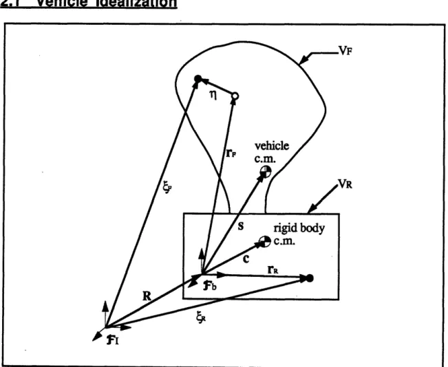
2.1 Vehicle Idealization

(24)

where

FI = inertial reference frame

Fb = body fixed reference frame VR = rigid body domain

VF = flexible body domain, reference configuration

4R(t) = material coordinate of rigid particle with respect to

inertial frame

4F(t) = material coordinate of flexible particle with respect to

inertial frame

R(t) = inertial position of body frame

rR = rigid particle position with respect to body frame

rF(t) = reference flexible particle position with respect to body frame

c = rigid c.m. with respect to body frame s(t) = vehicle c.m. with respect to body frame

rl(t) = displacement of flexible particle due to deformation

Figure 2.1 shows a rigid body with attached flexible appendage in inertial space. The form of the appendage is arbitrary, as suggested by the figure. In practice, the body fixed reference frame is located as a matter of convenience, and is not normally coincident with the rigid body c.m. or the vehicle c.m.

2.2 Principle of Virtual Work

The principle of virtual work is a statement that for a body in equilibrium under the action of prescribed body and surface forces the work done by these forces through a kinematically admissible displacement is equal to the change in internal virtual work. In combination with D'Alembert's principle, the virtual work principle can be expressed as

(25)

Chapter 2: Flexible Body Formulation

8Wext

=

f84.(f

-p)

dV +

fWint

8 t

dS =

e:o

dV =

(2.2.1) where, in addition to the quantities previously defined,

f = body force (force/volume) t = surface traction applied over So p = density

e = strain

a = stress

The virtual work statement is evaluated as the sum of two parts; integration over the rigid central body and integration over the flexible appendage.

2.3 Vectrix Notation

In forming the virtual work expression, several vectors must be defined. When the dynamic system involves more than one reference frame, as is the case for the vehicle of figure 2.1, it is helpful to use a notation which explicitly identifies the frame in which vector components are expressed. Toward this end, the vectrix notation [21] is used. A vector can be written as the multiplication of two column matrices: one containing the vector components, the other the frame unit directions. For example, an arbitrary vector v can be expressed in some reference frame

Fa,

whose basis vectors are al, a2, a3, as

S= + v3+ v 3

(26)

where

vT=-[ VI V2 V3

]

T

a- [- al a2 a3

Differentiation of vectors involving multiple reference frames introduces the vector cross product. It is convenient to express this operation as a matrix multiplication, in conjunction with vetrices. The cross product of arbitrary vectors u and v, both expressed in Fa, is given

by

UX

v = Tlra x

f a T=

Fa

( x _v)

(2.3.2)

where v is the same as above and the components of u have been formed into the skew symmetric matrix given by

0 -u3

u2

UX = u3 0 -ul

-u2 u1

0

1 _(2.3.3)

The inertial time derivative of the frame is also an important relationship and is given by

• T _T _T

(27)

2.4 Vehicle Kinematics

From figure 2.1, the inertial positions of rigid and flexible material particles are given by the vectors

R = R + rR (2.4.1)

4F = R + rF + 1

_(2.4.2)

Inertial accelerations are obtained through time differentiation of the position vectors. Let d( ) denote time differentiation

dt in the inertial frame,

indicate time differentiation in the body fixed frame. Differentiation of equation (2.4.1) gives

dR

d d rR]

dtLdt dt

_(2.4.3)

where it is convenient to let u = dR, the inertial velocity of the body fixed dt

frame. Now expressing components of u and drR in the body fixed frame dt

allows the derivative to be written as

(2.4.4) Application of the chain rule and using the vectrix notation gives the final form of the inertial acceleration of an arbitrary rigid material particle. The acceleration of an arbitrary flexible particle follows in an analogous manner. ,. T. _v . .. . " 1 . R = b LU + -" u + _" R + W _ rW ) =Yb

and

(')

aR _(2.4.5)

--R ••'bTrU +

b7

T

4

ýR=dt

_dt

_brI

(28)

Chavter 2: Flexible Body Formulation

F

-

vb

T + " x U + (x (rF + ) + 2o)x

1

+ ox (ox (rF+t) +

]

Virtual displacements are obtained through variation of the position vectors, and can be expressed as

SR = bT [8 + SW R _(2.4.7)

(2.4.8) where

rR,

r.

9F, = components of rR, rF, Ti, expressed in the body fixed

frame

ii = components of the body fixed frame

inertial velocity of the origin of the o = components of the inertial angular velocity of the body

fixed frame

8x

T

Tb

= components of the variation of inertial position vector R = components of angular variation which arises as a

consequence of rotation of the body frame with respect to the inertial frame

= components of the variation of the relative displacement vector Tj

S bl

b2 b3

All components defined above are expressed in the body fixed frame,

Fb. Note that the acceleration of a flexible particle has a high degree of

coupling between rigid body motions and flexible deformations.

(2.4.6)

(29)

2.5 Exact

Governing Equations

The governing equations of motion are obtained by substituting equations (2.4.5)-(2.4.8) into equation (2.2.1). Evaluation of equation (2.2.1) produces terms which can be grouped according to the variation (Sx, 8., or S1I) multiplying each. Because of the arbitrariness of the variations, each group must independently be equal to zero. Thus the following three sets of governing equations are obtained.

Recall that no restrictions have been imposed regarding the physical shape of the flexible appendage, or on the form of the relative

displacements 11.

Body Frame Translation (3SX):

(2.5.1)

Body Frame Rotation

(80):

f--T+fV

+

fF dV +

p(r

(r+tFdS = mcX

r

+ mef

jX

p

+

I -+

ox I + 2 p+•_ + lYW dV + prF + qdV F+ ff dV + tF dS = mi + mf . lu + mix C + mie _

+ 2Wf

pi

dV

+

fV

pi

dV

(2.5.2)

(30)

Flexible Appendage DOFs

(S3):

aRT

f dV

+

81T t dS = 81Tp dVfi + ₆_• _T p dVox u fFp

+

f

1T

*'F V W6x (rF + )p dV + 2

+

f8T

_

lx

(rEF+

)p

dV +

VF 8 T (ox ýp dV fvF where F = FB+ FT T = TB + TT

1 =

TR

+

TF

pdV + f

pdV p R dV + p(rF + dV( ₎ fvp

_(2.5.8)

PrRx tx rRdV

(2.5.9)

ox

IR

= IXRO - _P_rRx _WOx_{(_x}_{rR dV} fVR P(ER + 1fx x(rR + ~ dV

(2.5.11)

ip dV + 8c:o dV

(2.5.3)

(2.5.4)

(2.5.5)

(2.5.6)

m

= fVR

mc

= VR (2.5.7)

(2.5.10)

-F6 =

f

(31)

)X 1FO ) = p f

_

IF_=

[p(rF

+

• eo ex (rF + )

~

dV

V , (2.5.12)

along with the following definitions:

F = components of total force acting through body frame origin, due to body forces (EB) and surface

tractions (FT), expressed in the body fixed frame T = components of total torque acting about body frame

origin, due to body forces (TB) and surface tractions (IT), expressed in the body fixed frame

I = instantaneous inertia matrix of the vehicle about the body fixed frame due to rigid body (IR) and flexible body (IF),

expressed in body fixed frame

f.F = components of body forces acting on flexible body, expressed in body frame

tF = components of surface tractions acting on flexible body, expressed in body frame

m = total vehicle mass (mR + mF)

Equations (2.5.1)-(2.5.3) are an exact set of equations governing the idealized vehicle of figure 2.1. Discretization of the flexible domain stems from these equations. Two lumped parameter approximations will be considered: (a) discretization of the flexible domain into a collection of point masses (no rotatory inertia) interconnected by massless springs, and (b) extension of the previous model to include rotatory inertia.

In practice, mass is concentrated at locations corresponding to finite element nodes, which allows the use of the finite element stiffness matrix. For 3-D finite elements, condensation technique must be used to make the stiffness matrix compatible with approximation (a).

(32)

Finite element discretization can also be consistently applied to all integrals in Equations (2.5.1)-(2.5.3). Derivation is straightforward, but the solution procedure is more involved than lumped mass assumptions, and is therefore not considered here. This approach has been used to derive equations of motion and demonstrated through simple problems using quadratic beam elements [18].

2.6 Lumped

Mass

Assumption

ith mass particle ui

ri = ti = vi

-wi

Figure 2.2. Lumped mass discretization of the flexible appendage.

Schematic representation of this assumption is shown in figure 2.2, where the solid line represents the surface of the flexible appendage. The flexible domain is modelled with a finite number of point mass particles, connected by massless springs. Mathematically, this is a straightforward process whereby the integrals in equations (2.5.1)-(2.5.3) over the flexible domain are replaced by summations over the number of mass particles. The location of lumped masses correspond to the nodal locations of the finite element discretization of the flexible domain.

(33)

N

f

( ,

ý

i)p

dV -> If (qi,

f ,4 i mi

vi= _(2.6.1)

where

qi = ith nodal displacements (translations only), expressed in

the body fixed frame

mi = corresponding lumped mass

The motion of a lumped mass is fully described by three translations. For 3-D finite element models of the flexible domain which include rotations as nodal DOFs, condensation technique must be used to remove rotational DOFs from the stiffness matrix. Consistent with the lumped mass approximation, external loads on the flexible body are also 'lumped' at the nodes. The exact governing equations (2.5.1)-(2.5.3) are simplified through the lumped mass assumption to give

N N

E = mi

+ moxu + m6xc + m

cox c + 2

mi + mi Ii i= i=--1 (2.6.2) N T = mcx _{i + mc}x _ox _{u +}_{I 6} _{_+}_{wx I ) + 21 mi (ri + qij} x 4i i=l N + 1 mi

(r

+ qix qi i=1 _(2.6.3)

fi = _mii++ _mi _{+ mi.} x _{ri + jq_}+ _{miX W}

_(ri

_{+ _q)} + _{2miWx 4li}

N

+ mii + Kij qi i = 1,2,...,N

(34)

Chapter 2: Flexible Bodyv Formulation

where

ri = reference position of ith node, components in the body fixed frame

fi = lumped nodal forces

Kij = assembled stiffness matrix (rotation condensed out)

Equations (2.6.2)-(2.6.4) are valid for nonlinear flexible systems by interpretation of the stiffness matrix as the tangent stiffness matrix. An alternative derivation of the lumped mass equations of motion are provided in [22].

2.6.1 Equations of Motion

Equations (2.6.2)-(2.6.4) are the lumped mass equations of motion, comprising (6+3N) scalar equations. These equations can be recast into a single matrix equation of motion which can be numerically integrated.

MU + KU = R (2.6.5)

It is natural to partition the matrix equation into rigid and flexible body contributions and rewrite equation (2.6.5) as

MRR MRF

UR

0 0[

UR

RR

+RJ

MFR

MFF

UF

0 Kp

UF

RF

(2.6.6)

where

UR

4

(35)

Chapter 2: Flexible Body Formulation qi

A

N

m 0 0 m 0 0 0

mcx

ml ml ml mN mN mN S

0

0O

mi(ra + 2

(2.6.8) UF (3Nx1) MRR = (6x6) MFF (3Nx3N) MRF (6x3N) RR (6x1) mN -(2.6.11) (2.6.12) (2.6.9) (2.6.10) I- mcx _ox _-

_Ax

_{_I}

(36)

Chapter 2: Flexible Body Formulation RRF -(6x1) N -2y mio x _i i=l N

-21 mi(i + qi_ 4_i i=l RF= (3Nxl)

(2.6.13)

u - mlNx _{y• (II +}

_q9)

_-2_ml ₄₁

i

U - mNW W (rE + qjN - 2mNyx qN (2.6.14)

Note that the mass matrix M is symmetric, positive definite; the stiffness matrix K is symmetric, positive semi-definite and allows rigid body motion. Numerical solution can be obtained in a number of ways. For linear systems, transformation can be made to modal space, which allows truncation of both system size and high frequency modes. Modal reduction is generally not possible for nonlinear flexible systems. Thus direct integration is preferred in.the present context. Also the effect of various terms can be more readily assessed in physical space.

The methods available for direct integration of equation (2.6.5) can be classified into explicit and implicit schemes. Explicit schemes are conditionally stable and require very small time steps to integrate the highest frequencies accurately [23, 24]. Implicit schemes are advantageous because they are unconditionally stable and the step size can be chosen on the basis of accuracy only. This generally allows a much larger step size than would be required by explicit schemes. Because of the relaxed integration step size afforded by unconditionally stable implicit schemes, the Newmark integration method is implemented in the examples of chapter 5. Details of the Newmark scheme are outlined in Appendix B.

(37)

2.7 Lumped

Mass/Inertia

Assumption

ith nodal body

Figure 2.3. Lumped mass/inertia discretization of flexible appendage.

As in the previous derivation, integrals over the flexible domain are replaced by summations over a finite number of nodes. The nodes are now treated as small rigid bodies; they are no longer mass particles, but have both mass and inertia. Six quantities are required to describe the motion of each node.

Massless springs connect the nodal bodies just as in section 2.6. In practice, the finite element stiffness matrix provides information regarding interconnecting forces. The lumped mass/inertia formulation, as constrasted with the lumped mass formulation, has the advantage that finite element DOFs are used directly; no condensation is required in the numerical solution.

(38)

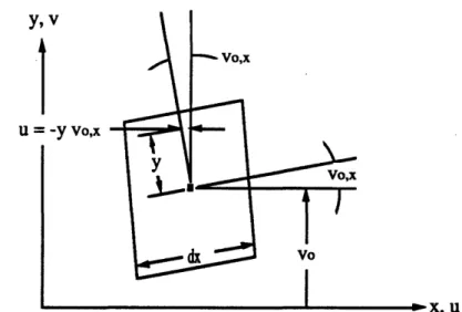
2.7.1 Kinematic

Description

undeflected configuration deflected configuration

Figure 2.4. Relative displacement of ith nodal body.

Consider the rigid nodal body shown in figure 2.4 with an arbitrary material particle labelled "a" in the undeflected configuration, "A" in the deflected configuration. As measured with respect to the body fixed frame, the nodal body undergoes infinitesmal translation and rotation in moving to the deflected configuration. The location of an arbitrary material particle in the undeflected configuration is given by

rF = _{rFo + 3X} _(2.7.1)

where rFo is the location of the nodal body reference frame in the undeflected configuration. The nodal body reference frame is aligned with the body fixed reference frame in the undeflected configuration.

(39)

In the deflected configuration, the location of A is given by

RF = RFo + A = rFo + qt + A . (2.7.2)

where RFo is the location of the nodal body reference frame in the deflected configuration. The relative displacement undergone by a material particle in moving from a to A is then

S= RF - rF = qt + A - (2.7.3)

Rotation of the nodal body reference frame can be expressed by the

skew symmetric infinitesmal rotation matrix so that

A = CX (2.7.4)

where

1 -Oz 0y

C

=

ze 1 -0x

-0y Ox

1

Substitution of equation (2.7.4) into (2.7.3) leads to expression of the relative displacement as

r = qt + CX - X = qt + (C - I)X _(2.7.5)

where I is the identity matrix. Now since all vectors are expressed in the body fixed frame, the component notation is adopted. The matrix (C -I) above can be compared with the skew symmetric matrix (associated with vector cross products) introduced in section 2.3. Define

(40)

Ox

Oz

so that qrx _{= (C - I). Finally, the relative displacement of a material}

particle, assuming infinitesmal rotation, can be written as

11 = qt + qrx _(2.7.6)

2.7.2 Equations of Motion

The equations of motion follow from substitution of equation (2.7.6) into equations (2.5.1)-(2.5.3) and evaluating. Reduction of the exact equations is complicated somewhat by the form of the relative displacement given by equation (2.7.6). Some integrals produce higher-order terms which cannot be given simple physical interpretation. These higher-order terms are ignored. Details of integrations are not presented, and the lumped mass/inertia equations of motion in matrix form are given by

MRR

MRF

R

0

0 UR

RR

+

RRF

M MFF -UJ

U

0 K J UF RF (2.7.7)

where all partitions are explicitly defined below. Note that the rigid-rigid partition is the same as in section 2.6. KFF is the full stiffness matrix produced by the finite element method. The tangent stiffness matrix is used for the solution of problems with nonlinear flexibility.

UR

F

(41)

Chapter 2: Flexible Body Formulation UF (6Nxl) MRR (6x6) MFF (6Nx6N) MRF --(6x6N) tli qrl itN qrN m 0 0 0 m 0 0 0 ml ml ml(rL + q (2.7.9) (2.7.10) mN mN mN

IN

-mN (2.7.11) mN mN

mN(rN + q

_IN (2.7.12)

(42)

-Chapter 2: Flexible Body Formulation

RR

[

F - mfX u - m-x ox c

(6x1)

T - mcx

c

x

_u

_-

_OX

_1J

_(2.7.13)

RR_F( (6xl) RF= (6Nxl) N i=1

-2 mie q'

N N -21 mi(ri + e M + i1 e iik . i=l1 i=l1 _(2.7.14)

fi - ml u - mi~x Wx (rL + t) -" 2mix qt + h.o.t.

t_ + h.o.t.

fN- mN

- mNmNW

CM N +

-tN)"

2mNx qltN + h.o.t.

tN

+

h.o.t.

(2.7.15)

2.8 Extending Symbolic Rigid Body Codes

Implementation of the flexible body formulation can take advantage of available symbolic rigid body software. These software packages produce FORTRAN coding of the equations of motion of a user specified rigid multibody system. Some examples of symbolic manipulation rigid multibody software include SD/FAST [25], AUTOSIM [26], and AUTOLEV [27]. The use of symbolic rigid body codes allows the analyst to concentrate on a smaller set of 'hand derived' equations addressing the flexible domain [28, 29].

To show how the rigid body subroutines, generated by any one of the above programs, can be used in the flexible body implementation, the

(43)

partitioned equations of motion (2.6.6) or (2.7.7) are rewritten as a pair of matrix equations

U

UR+ MRF F =F + RRF (2.8.1a)

MFR UR + MFF UF + KFF UF = RF (2.8.1b)

where it is noted that MRR and RR refer to the current configuration of the

vehicle, i.e the rigid body + flexible appendage is assumed rigid in the

current configuration.

The rigid body code produces a set of subroutines to solve the rigid equations of motion

MRR UR = RR (2.8.2)

2.8.1 For Second Order Integration Schemes

When a second order integration scheme is used in the solution of the vehicle equations of motion, the rigid subroutine is necessary only in the calculation of MRR and RR. The current configuration vehicle c.m. and inertia matrix are provided as inputs to the subroutine. If the vehicle undergoes large flexible displacements, the configuration must be updated at each integration step.

(44)

Chaoter 2: Flexible Body Formulation

2.8.2 For First Order Integration Schemes

A sketch of the implementation of a Runge-Kutta integration scheme in the solution of the equations of motion is offered in Appendix B. It is shown that the computational effort is concentrated on the evaluation of derivatives, in order to employ the formula given by equation (B.4.3). In section B.5, equations (2.8.1) are rearranged to yield

[MRR - MRF MFF-1 _MFR] _R₌_{RR + RRF +...}

(B.5.4)

and

UF = MFF- 1 _[RF

- MFR UR - KFF UF] _(B.5.3)

To obtain the derivatives UR and UF, these two equations must be solved in the order given. Examination of equation (B.5.4) indicates that the code produced to solve equation (2.8.2) can be used in the flexible context by modification to MRR and RR. Simulations using first order integration schemes can take advantage of the code produced by symbolic software to a larger extent than simulations using second order schemes.

(45)

Chapter 3: Derivation of Finite Elements

Chapter 3 Derivation of Finite Elements

This chapter presents the derivation of two nonlinear beam finite elements. Isotropic, prismatic beam elements are allowed to stretch, bend in two planes, and undergo St. Venant torsion. For the Timoshenko beam, shearing in two planes is also allowed. To derive the beam finite elements, assume that the flexible domain of chapter 2 (see figure 2.1 and equations (2.5.1)-(2.5.3)) is a beam, which allows explicit statement of kinematic assumptions. Bernoulli-Euler kinematic assumptions comprise the "engineering theory of beams." A distinction is made between Bernoulli-Euler and Rayleigh beam theories in dynamics (Bernoulli-Bernoulli-Euler ignores rotatory inertia). The Timoshenko kinematic assumptions lead to a beam theory which includes the effects of rotatory inertia and shear strain within the beam.

The development proceeds from the 3-D statement of the principle of virtual work. Kinematic assumptions are explicitly introduced, and the work expression is integrated across the beam cross-section area for reduction to a 1-D theory.

The beam elements derived are generally known as 'isoparametric' elements; isoparametric meaning 'same parameters'. For the current discussion, let element geometry be interpolated from nodal values by using shape functions. Let element displacements be interpolated from nodal DOFs by using interpolation functions. Strictly speaking,

(46)

Chapter 3: Derivation of Finite Elements

isoparametric formulations employ the same function for shape and interpolation. It should be noted that although the C1 _{element to follow}

does not adhere to this rigorous definition (it uses both linear and cubic interpolation functions), it may be loosely referred to as isoparametric. The CO _{element is a true isoparametric element.}

3.1 Principle of Virtual Work

The principle of virtual work has been previously stated in section 2.2, where it was applied to a vehicle composed of rigid central body and attached flexible appendage. Three coupled sets of integral equations were derived which govern the vehicle motion. Equations (2.5.1) and (2.5.2) govern the translation and rotation of the the rigid body. Equation (2.5.3) governs the deflections of the flexible appendage, relative to the body fixed frame. For the purpose of this derivation, consider the rigid body to be fixed in inertial space, i.e. a = q = 0. Thus surviving terms give the

virtual work expression which governs the deflections of the beam relative to a body fixed reference frame.

&nTfE

dV +

5tE dS

=

T

ITp

dV +

Be:a

dV

(3.1.1) where

11 = components of flexible displacement, with respect to the body fixed frame

fF = force/unit volume, with respect to the body fixed frame IF = surface traction applied over Soy, with respect to the body

(47)

p = density

VF = reference configuration of the flexible body

e = strain

a = stress

3.2 Beam Theory Preliminaries

y, v X. U

1', W

Figure 3.1. 3-D Beam Coordinate System.

Consider the beam shown in figure 3.1, with coordinate axes as shown. It is assumed that stresses ay and dz are small compared to ox. St. Venant torsion theory is incorporated into the displacement field (sections undergo zero warping, and there is no distortion of the cross-section). The displacement field associated with the Bernoulli-Euler kinematics are

u(x,y,z) = uo(x) - yvo,x(x) - zwo,(x)

v(x,z) = Vo(X) -

zOx(x)

(3.2.1)

w(x,y) = wo(x) + y0x(x)

and can be interpreted geometrically to mean that cross-sections remain perpendicular to the neutral axis during deformation. A representative construction is shown in figure 3.2.

(48)

ChQpter 3: Derivation of Finite Elements

y, v

u = -y vox

U = -y Vo,x

Figure 3.2.. Kinematics of Bernoulli-Euler Beam Theory.

In the Timoshenko beam theory, cross-sections initially perpendicular to the neutral axis of the beam remain plane but not perpendicular to the neutral axis during deformation. This kinematic

assumption is shown geometrically in figure 3.3.

y, v

u = -y Oz

Figure 3.3. Kinematics of Timoshenko Beam Theory.

" " ,xll

(49)

Chanter 3: Derivation of Finite Elements

The displacement field associated with the kinematics of Timoshenko beam theory.are

u(x,y,z) =

uo(x)

-

y0z(x)

+

z0y(x)

v(x,z) = vo(x) -

z0x(x)

_(3.2.2)

w(x,y) = w(x) +

y0x(x)

where zero subscripts indicate displacement of the neutral axis and O's are rotations about the subscripted axes.

Note the difference in sign of the components in the displacement field u(x,y,z) of Bernoulli-Euler and Timoshenko kinematics. Positive rotation associated with w,x disagrees with the right hand rule, and as a consequence, also disagrees with the right handed coordinate system used in the derivation of the vehicle equations in chapter 2. Therefore, in order to use the Bernoulli-Euler (Cl) element in the dynamic simulation, a transformation must be made so that the rotation is consistent with a right hand coordinate system.

The restriction of zero deformation of the cross-section during torsion implies that yyz = 0. The assumptions associated with both kinematic models allow reduction of the 3-D linear elastic, isotropic

stress-strain relations to the simple result

E

Ox

Ex

xy

=

G

_Yxy

(50)

Chapter 3: Derivation of Finite Elements

3.3 C

1

_Formulation

The C1 _{formulation encompasses both the Bernoulli-Euler and}

Rayleigh beam theories. The subtle distinction is the inclusion of rotatory inertia in Rayleigh's equations governing the motion of a beam [30]. It will be shown that consistent derivation using the virtual work principle produces the Rayleigh theory. By convention, Bernoulli-Euler theory excludes rotatory inertia.

From small deflection theory, the non-zero strains associated with the displacement field of equation (3.2.1) are

Ex = u, = Uox(X) - yvo,xx(x) - zwo0,(x)

Yxy =

,y

+ V,x = - ZOx,x(X) _(3.3.1)

Yzx = w, +

u,

=

y0x,x(x)

Substituting equations (3.3.1) and (3.2.1) and constitutive relations (3.2.3) into the right hand side of (3.1.1) gives the internal virtual work expression in the volume integral form

•V

p[(Suo - yvo,x -z8wox)

(iio

-yvo, - zwo,x) + (8vo -zx) (vo -zix)

+ (Swo + y80x)

(wo

+ y~x)]

+ E(Buo, - yavoxx -

z8wo,xx) (uO,x

- yvo,xx - zwo0 x)

+ G(-z80x,) (-zOx,) +

_{G(ySOx,x) (yex,x)) dV}

=

RHS

(3.3.2)

where the domain is understood to be the flexible volume. The expression (3.3.2) can be integrated through the beam cross-section to give

(51)

i

{m(uoiio

+

8vo

0

o +

wowo)

+ (Imy

+ Imz)808,x

+ ImyGWo,xWo,x + ImzBVo,xVo,x + EA8uo,xuo,x

+ EIy•Wo,xxWoxx + EIz8vo,xxvo,xx

+

G(Iy

+

Iz)80x,xox,x)dx

=

RHS

(3.3.3)

where cross-section principal axes are assumed to be aligned with element coordinate axes. Constants appearing in equation (3.3.3) are defined as follows:

A= dA

m= pdA

Iy= z2dA Iz •Y2dAJ= +I,

Imy = pz2dA Imz =PY2dA

where

SydA

=fzdA = yzdA =

0

m = mass/length

Iy, Iz = area moment of inertia Imy, Imz = mass moment of inertia

The integral equation (3.3.3) appearing above is to be evaluated over the length of the flexible domain. The flexible domain is decomposed into finite elements and equation (3.3.3) becomes a summation of integrals over the individual element domains. The continuity of assumed displacement functions is dictated by the terms appearing in the integrand. Since second

(52)

derivatives of displacement exist in the element stiffness integral, inter-element continuity requires that the displacement fields wo and vo be C1 continuous. The axial displacement and twist require only CO continuity. (The superscript indicates the derivative through which the function or field is continuous.) The continuity condition is the integrability of equation (3.3.3) over the entire domain.

3.3.1 Discretization

5=-1 }-H= =+1

Node Node

1

2

Figure 3.4. Local coordinates for 2 node beam element.

The two node element is defined by the local coordinate system shown in figure 3.4. The element has six DOFs at each node. The necessary interpolation functions are defined in terms of the local coordinate 5. The linear interpolation functions are given by

No, = 1 (1

-•)

2

N = L _{(1 + 5)}

2 _(3.3.4)

For the C1 continuous displacement fields wo and vo, the cubic Hermitian interpolation functions are used and are defined as