High-resolution images of diffuse neutral clouds in the milky way. Ⅰ. observations, imaging, and basic cloud properties

(1)

Publisher’s version / Version de l'éditeur:

Vous avez des questions? Nous pouvons vous aider. Pour communiquer directement avec un auteur, consultez la première page de la revue dans laquelle son article a été publié afin de trouver ses coordonnées. Si vous n’arrivez pas à les repérer, communiquez avec nous à [email protected].

Questions? Contact the NRC Publications Archive team at

[email protected]. If you wish to email the authors directly, please see the first page of the publication for their contact information.

https://publications-cnrc.canada.ca/fra/droits

L’accès à ce site Web et l’utilisation de son contenu sont assujettis aux conditions présentées dans le site LISEZ CES CONDITIONS ATTENTIVEMENT AVANT D’UTILISER CE SITE WEB.

The Astrophysical Journal Supplement Series, 219, 2, p. 16, 2015-08-01

READ THESE TERMS AND CONDITIONS CAREFULLY BEFORE USING THIS WEBSITE. https://nrc-publications.canada.ca/eng/copyright

NRC Publications Archive Record / Notice des Archives des publications du CNRC :

https://nrc-publications.canada.ca/eng/view/object/?id=cdc4b62b-78ac-4e0c-9567-8eddfc17dfd4

https://publications-cnrc.canada.ca/fra/voir/objet/?id=cdc4b62b-78ac-4e0c-9567-8eddfc17dfd4

This publication could be one of several versions: author’s original, accepted manuscript or the publisher’s version. / La version de cette publication peut être l’une des suivantes : la version prépublication de l’auteur, la version acceptée du manuscrit ou la version de l’éditeur.

For the publisher’s version, please access the DOI link below./ Pour consulter la version de l’éditeur, utilisez le lien DOI ci-dessous.

https://doi.org/10.1088/0067-0049/219/2/16

(2)

HIGH-RESOLUTION IMAGES OF DIFFUSE NEUTRAL CLOUDS IN THE MILKY WAY. I.

OBSERVATIONS, IMAGING, AND BASIC CLOUD PROPERTIES

Y. Pidopryhora1,4, Felix J. Lockman2,6, J. M. Dickey1, and M. P. Rupen3,5,6

1

School of Physical Sciences, University of Tasmania, Private Bag 37, Hobart, 7001, Tasmania, Australia;[email protected]

2

National Radio Astronomy Observatory, Green Bank, WV 24944, USA;[email protected]

3

National Radio Astronomy Observatory, Socorro, NM 87801, USA;[email protected]

4

Argelander-Institut für Astronomie, Auf dem Hügel 71, D-53121, Bonn, Germany;[email protected]

5_{Dominion Radio Astronomy Observatory, National Research Council, P.O. Box 248, Penticton, BC, V2A 6J9, Canada} Received 2014 December 23; accepted 2015 June 10; published 2015 July 28

ABSTRACT

A set of diffuse interstellar clouds in the inner Galaxy within a few hundred parsecs of the Galactic plane has been observed at an angular resolution of ≈1′. 0 combining data from the NRAO Green Bank Telescope and the Very Large Array. At the distance of the clouds, the linear resolution ranges from ∼1.9 to ∼2.8 pc. These clouds have been selected to be somewhat outside of the Galactic plane, and thus are not confused with unrelated emission, but in other respects they are a Galactic population. They are located near the tangent points in the inner Galaxy, and thus at a quantiﬁable distance: 2.3⩽R⩽6.0kpc from the Galactic Center and -1000⩽z⩽+610pc from the Galactic plane. These are the ﬁrst images of the diffuse neutral HIclouds that may constitute

a considerable fraction of the interstellar medium (ISM). Peak HIcolumn densities lie in the range NHI = 0.8–2.9 × 10

20

cm−2_{. Cloud diameters vary between about 10 and 100 pc, and their H}_I_{mass spans the}

range from less than a hundred to a few thousands Me. The clouds show no morphological consistency of any

kind, except that their shapes are highly irregular. One cloud may lie within the hot wind from the nucleus of the Galaxy, and some clouds show evidence of two distinct thermal phases as would be expected from equilibrium models of the ISM.

Key words:_{Galaxy: disk – ISM: atoms – ISM: clouds – ISM: general – ISM: structure – radio lines: ISM}

1. INTRODUCTION

The concept of a diffuse interstellar cloud is more than 50 years old, yet there are few observations that support the most basic aspects of the standard picture. The strongest evidence for discrete clouds is kinematic: there are usually distinct absorption lines at different velocities in spectra toward stars (e.g., Munch 1952; Hobbs 1978; Redﬁeld & Linsky

2008). However, spectral features can be produced not only by spatial structures, i.e., clouds, but also in a continuous turbulent medium(Lazarian & Pogosyan2000). In contrast to the often well-deﬁned clouds of molecular gas, like the Infrared-dark Clouds (e.g., Rathborne et al.2010), there is little support for the existence of discrete clouds in 21 cm emission observations, which suggest instead that the atomic interstellar medium (ISM) consists of fragments of ﬁlaments and “blobby sheets,” many of which may be a consequence of turbulence(Kulkarni & Heiles 1987; Dickey & Lockman 1990; Heiles & Troland

2003; Miville-Deschênes et al.2003; Kalberla & Kerp 2009). In most directions, 21 cm HIemission maps are highly

confused, leading to considerable ambiguity when determining the morphology and boundries of interstellar clouds, even assuming that they do exist. A massive study of NaI and CaII

absorption lines toward nearly 2000 stars within 800 pc of the Sun by Lallement et al. (2003) and Welsh et al. (2010) has revealed the three-dimensional structure of the local ISM, “cell-like cavity structures,” a fragmented “wall” of neutral gas, and what appears to be clouds “physically linked to the wall of denser gas,” but it is difﬁcult to know how to generalize this result to the broader ISM.

The situation is quite different, however, in the lower halo of the inner Galaxy where there is a population of discreet HIclouds whose velocities are consistent with circular rotation,

but whose location several hundred parsecs from the area separates them from unrelated emission (Lockman 2002,

2004).7 Similar clouds can be seen at low Galactic latitude when their random velocity is large enough to remove confusion (Stil et al. 2006); others are detected in the outer Galaxy(Stanimirović et al.2006; Strasser et al.2007; Dedes & Kalberla2010). The clouds in the inner Galaxy are likely the product of HIsupershells as their abundance and scale height

are linked to the large-scale pattern of star formation in the disk (Ford et al.2008,2010).

While many aspects of these “disk-halo” clouds are poorly understood, they can be used as test particles sensitive to the physical conditions in their surroundings, and thus give information about interstellar processes not easily obtained from the highly blended spectra typical of most observations. The disk-halo clouds in the inner Galaxy are so abundant that a number of them lie near the terminal velocity in their direction, and thus near the tangent point, whose distance is determined from simple geometry. Their locations, masses, and sizes can be estimated with quantiﬁable errors.

There have been numerous theoretical studies of the expected properties of the diffuse ISM as a function of location in the Galaxy, distance from the Galactic plane, sources of heating, etc. Strong theoretical predictions have been made, especially about the existence of two thermal phases in pressure

6

The National Radio Astronomy Observatory is a facility of the National Science Foundation operated under a cooperative agreement by Associated Universities, Inc.

7 _{First detections of a few prominent representatives of this population date}

back to Prata(1964), Simonson (1971), and Lockman (1984). A very detailed history and bibliography of both observational and theoretical early studies of interstellar clouds and HIhalo can be found in Chapter 1 of Pidopry-hora(2006).

(3)

2. SELECTION OF TARGETS

Targeted 21 cm HI surveys of regions in the inner Galaxy

made with the GBT have provided a list of diffuse clouds that might be suitable for high-resolution imaging (Lock-man 2002, 2004). From these, we selected a set using the following criteria: (1) the clouds have LSR velocities at or beyond the terminal velocity in their direction, ensuring that their distance could be determined (see Section 2.1); (2) the clouds cover a range of Galactic longitude and latitude, ensuring that different environments were probed, although all are in the ﬁrst quadrant of Galactic longitude; (3) the clouds are relatively isolated in position and velocity to minimize potential confusion; and(4) their 21 cm emission as observed with the GBT is bright enough to be detectable with the VLA in a few hours. An example of the GBT observations used to select the clouds is given in Figure1. Table 1gives the cloud designation, ﬁeld center, and the 21 cm line peak brightness temperature, FWHM, and velocity as determined from the GBT observations.

2.1. Distance

The kinematics of the disk-halo cloud population studied here are dominated by the circular rotation of the Milky Way with a cloud–cloud velocity dispersion of σcc≈

16 km s−1_(Lockman ₂₀₀₂_{; Ford et al.} ₂₀₀₈_, ₂₀₁₀_{). Toward}

the inner Galaxy, the maximum velocity permitted by Galactic rotation at b= 0° is referred to as the terminal velocity, Vt, and

arises from the tangent point where the distance from the Galactic Center is Rt=R0 sinℓ. Here, we use R0= 8.5 kpc,

the IAU recommended value(Kerr & Lynden-Bell1986). The terminal velocity can be measured from observations of species such as HIor CO, or can be approximated with a rotation curve

(e.g., Clemens 1985; Burton & Liszt1993; McClure-Grifﬁths & Dickey2007; Dickey2013). In the ﬁrst quadrant of Galactic longitude, Vt > 0 and an object with VLSR Vt thus must lie

near the tangent point where its distance is known from geometry. In the current sample, all clouds have velocities

VLSR Vt, and so we calculate the tangent-point distance

projected on the Galactic plane as dp=R0 cosℓ. A cloud’s

distance from the Galactic plane is then z =dptanb and the

distance to the cloud center isd (dp2 z2)

1 2

= + .

errors as well as the distance of each cloud from the Galactic plane.

3. OBSERVATIONS AND BASIC DATA REDUCTION

3.1. Green Bank Telescope Observations

The GBT was used to map HIemission around the disk-halo

clouds to measure their overall properties, to determine whether they might be suitable for high-resolution imaging, and to provide the short spacing data for image reconstruction (see, e.g., Stanimirović et al.1999). Maps were made over an area around each cloud of 1◦_{. 5 × 1}◦_{. 5 or 2° × 2° depending on the}

extent of the cloud. Spectra were taken every 3′. 5 in Galactic longitude and latitude, which is somewhat ﬁner than the Nyquist sampling interval for the GBT’s 9′. 1 beam (FWHM). Observations were repeated several times over a period of a few months. In-band frequency switching provided a useable velocity coverage of 400 km s−1_{around zero velocity}_{(LSR) at}

a channel spacing of 0.16 km s−1_.

3.2. Very Large Array Observations

A sample of 20 HIdisk-halo clouds was observed in 21 cm

line emission spectroscopy with the VLA in D conﬁguration during 2003 and 2004. The spectra had 256 frequency channels separated by 0.64 km s−1_{in equivalent Doppler velocity}

centered on the peak velocity of each cloud (Pidopryhora et al.2004; Lockman & Pidopryhora2005; Pidopryhora2006). Fifteen of the clouds were observed in single pointings, and five as mosaics. Two of these were also observed in C configuration with the identical spectroscopic setup (Pidopry-hora et al. 2012) and two more (G21.2+2.2 and G35.6+3.9) were observed in B configuration at both HIand OH

frequencies in an attempt to detect absorption against bright background continuum sources. Here, we present results for just the 10 clouds observed only in D conﬁguration with single pointings, deferring discussion of the others to a later paper. Parameters of the VLA observations are provided in Table2. An example of the uv coverage for one of the clouds is given in Figure2.

3.3. Green Bank Telescope Data Reduction

The spectra were calibrated and corrected for stray radiation as described in Boothroyd et al. (2011), and a second-order polynomial was ﬁt to emission-free regions of each spectrum to correct for residual instrumental effects. For each cloud, the

(4)

data were assembled into a cube on a 105″ grid. There was occasional narrow-band interference that was stable in frequency, and so spectra were interpolated over the affected channels. The ﬁnal GBT data cubes had a brightness temperature noise ≈0.1 K in a 0.16 km s−1 _channel.

Each GBT image cube was converted to the same coordinate system as the VLA, cropped to ﬁt the exact VLA ﬁeld size, and interpolated to the matching grid and sequence of spectral channels with the Miriad(Sault et al.1995) task REGRID. The GBT data were taken while the telescope was moving, and thus

have an effective resolution of ≈9′. 6 × 9′. 1 with the major axis along Galactic longitude, that is, the scanning direction. In the VLA’s equatorial coordinate system, this resulted in slightly different beam position angles for each ﬁeld. In order to smooth out gridding artifacts, each GBT image was also convolved with a circular beam function of 200″, approximately 1/3 of the original beam size, and so the ﬁnal GBT angular resolution is approximately 10′ FWHM.

3.4. Very Large Array Data Reduction

After calibration and study of preliminary dirty images of each VLA ﬁeld, the continuum was subtracted in the uv domain using the AIPS UVLIN task based on selected line-free channels. Naturally weighted dirty images of continuum-free data were then cleaned channel by channel with AIPS SDCLN with no cleaning mask applied. The residual ﬂux threshold was set to 0.7 mJy beam−1

for all clouds, corresponding to 0.2–0.3 σ. In the ﬁnal step, the correction for the VLA primary beam was applied to the clean image cubes with the AIPS task PBCOR. The imaging synthesized beam size was different for each ﬁeld as described below; their values are given in Table3.

4. FURTHER DATA PROCESSING, NOISE LEVELS, AND ERRORS

4.1. Combining the Interferometric and Single-dish Data

For several reasons, we have chosen to use Miriad’s IMMERGE to combine the interferometric and single-dish data: (1) it uses a well-understood algorithm that is easy to control;(2) it runs quickly and is easily applied to large image cubes; and (3) we have developed a calibration technique described below that ensures the accuracy of the results.

Another approach was also tried for two clouds which are not of the set described in this paper(Pidopryhora et al.2012): using a maximum entropy (MEM) algorithm (AIPS VTESS task) with the GBT image used as the default, but it was found to be less efﬁcient. For a detailed review of all possible methods see Stanimirović(1999).

Miriad’s task IMMERGE uses a linear method sometimes known as “feathering” to combine interferometric and single-dish data (Stanimirović 1999; Sault & Killeen 2011). Essen-tially, this is just merging clean interferometric and single-dish images after Fourier-transforming them into the uv domain, the result covering the whole combined spatial frequency range. For this procedure to be meaningful the Fourier images of interferometric and single-dish data should match within the overlapping ranges of their common spatial frequencies. Due to the completely different natures of the two original data sets, and thus the unavoidable discrepancies, this has to be ensured by varying their common calibration scaling factor fcal, which is

the main control parameter of the IMMERGE task. In the case that the calibration of both data sets was done properly, this factor should be close to unity but its exact value has to be determined empirically in each particular case. If a compact source of 21 cm emission were present in the ﬁeld of view, both unresolved by the VLA and unconfused with other emission by the GBT, then determining fcalwould be as simple as dividing

the interferometric ﬂux density of this source by its single-dish ﬂux density. Unfortunately, such sources are rare and not present in our data, so a more complex strategy of determining

fcalwas used.

Figure 1. Velocity-latitude image of HIemission from GBT observations after Lockman & Pidopryhora (2005). The cloud at 24.3–5.3 is marked with an arrow. The expected maximum VLSRfrom Galactic rotation (Clemens1985) is

marked by the slightly curved vertical line. The location of G24.3−5.3 slightly beyond the maximum velocity indicates that it must lie near the tangent point in its direction. Note that it is separated in position and velocity from other HIemission and is thus relatively unconfused.

Table 1

Cloud Properties from GBT Observations

Name Tb VLSR FWHM Distance z (K) (km s−1₎ _{(km s}−1₎ _(kpc) _(pc) (1) (2) (3) (4) (5) (6) G16.0+3.0 1.1 +143 5.4 8.2± 1.0 +430± 50 G17.5+2.2 1.6 +139 16.2 8.1± 1.1 +310± 40 G19.5–3.6 3.5 +121 13.1 8.0± 1.6 −500 ± 100 G22.8+4.3 3.1 +137 7.8 7.9± 1.4 +590± 100 G24.3–5.3 1.3 +124 13.5 7.8± 1.5 −720 ± 140 G24.7–5.7 1.8 +127 8.9 7.8± 1.5 −770 ± 150 G25.2+4.5 2.6 +147 10.4 7.7± 1.6 +610± 130 G26.9–6.3 3.4 +123 8.8 7.6± 1.7 −840 ± 190 G33.4–8.0 1.1 +102 5.5 7.2± 2.0 −1000 ± 280 G44.8–7.0 3.3 +94 9.0 6.1± 2.5 −740 ± 300

(5)

There is another important control parameter called “taper-ing.” If IMMERGE tapering is applied, then the Fourier image of the interferometric data is smoothly continued into the low spatial frequency region (Sault & Killeen 2011). This ﬁxes

possible edge effects in the Fourier transformation but introduces an additional nonlinear distortion of the data. In addition to determining the best value of fcal, it is necessary to

decide whether or not tapering should be applied.

4.2. Derivation of the Optimal fcal

IMMERGE has a built-in method of matching the two data sets and deriving fcal, provided that the overlapping range of

spatial frequencies is deﬁned. Figure 3 shows examples of application of this method. The interferometric image is convolved with the single-dish beam, then both images are Fourier-transformed and compared to each other within the overlapping spatial frequency range. The value of fcalis

selected by scaling the single-dish data until the slope of the line fit to the data is exactly 1. Based on several trials varying IMMERGE parameters with different samples taken from our data, we have determined that(1) tapering distorts the data and makes a reasonable linear fit impossible, and (2) due to a large scatter of the values, the best linear fit usually does not characterize the data well and fcalderived from it should be

treated only as an estimate. Thus, for our purposes, we use IMMERGE without tapering and we determine the optimal

fcalby other methods.

It should be noted that describing the discrepancy between single-dish and interferometric data with a single linear parameter is only an approximation of very complex behavior. One immediately notes that the optimal fcalseems to be

different for different channels (Stanimirović 1999). In particular, it is sensitive to the signal-to-noise ratio and spatial signal distribution of brightness in each channel. This is understandable as fcalshould ideally be determined from a point

source unresolved by both telescopes. For a cloud comprised of diffuse gas that smoothly ﬁlls the ﬁeld of view and is detectable by the single-dish but is completely invisible to the interferometer, the estimated fcalapproaches zero. In the cloud

data, we usually have some combination of these two extreme cases, and what seems to be the optimal fcalmay ﬂuctuate

signiﬁcantly. However, allowing it to vary with frequency would introduce an unknown nonlinear distortion. Based on the general assumptions of this model, and as all clouds observed only with the VLA D-array present the same variety of interferometric data (similar beam sizes, noise levels, uv coverage, etc.), we sought a single value of fcalthat would work

well not only for every channel of a particular cloud, but for all 10 clouds.

Figure 2. uv coverage of the VLA observations of one of the clouds, G26.9−6.3. Two epochs of 2004 June 29 and July 24 combined, total integration time 215 minutes, source declination δ ≈ −8°.

Table 3 Synthesized Beam Sizes

Cloud FWHM Gain áFWHMñ (″) (K Jy−1₎ _(pc) G16.0+3.0 89.5 × 52.6 129 2.7 G17.5+2.2 85.7 × 56.5 126 2.7 G19.5−3.6 84.6 × 58.0 124 2.7 G22.8+4.3 72.9 × 56.1 149 2.4 G24.3−5.3 75.6 × 56.2 143 2.5 G24.7−5.7 77.0 × 59.8 132 2.6 G25.2+4.5 71.2 × 55.6 154 2.4 G26.9−6.3 73.5 × 57.3 145 2.4 G33.4−8.0 73.0 × 58.3 143 2.3 G44.8−7.0 68.5 × 57.7 154 1.9

(6)

One criterion for testing the goodness of a particular value of

fcalis that the spectrum of the merged cube averaged over an

area somewhat larger than the GBT beam, but small enough not to be effected by the VLA primary beam pattern, should match the average taken over the same region in the single-dish data alone. We have found that averaging over an area 15′. 3 × 15′. 3 at the center of the field works well for all clouds observed with the VLA D-array. Requiring that the average spectrum over this area given by IMMERGE matches the single-dish mean profile is sufficient to derive an optimal fcal = 0.87. In fact, this

method may be preferable to any other since it directly preserves the single-dish ﬂux.

Figure4shows the comparison of mean line proﬁles of the VLA, the GBT, and the best IMMERGE combined images for all 10 targets using the single value of fcal = 0.87, which was

adopted for all subsequent work.

4.3. Testing the Accuracy of the Image Produced by IMMERGE

The average difference between the observed GBT and ﬁnal IMMERGE line proﬁles can be calculated as

(

)

D P i P i P i ( ) ( ) ( ) , (1) i i GBT IMMERGE GBT

å

á ñ =

-where PGBT(i) and PIMMERGE(i) are the spectral values for

individual channels and the summing is done over velocities of interest for each cloud. Figure5shows values ofá ñ for all 10D

clouds. Taking into account the peculiarities of proﬁles that make their exact match impossible, e.g., the presence of large amounts of Galactic diffuse gas invisible to the interferometer as in clouds G33.4−8.0 and G44.8−7.0, these values set an

upper limit to the error possibly introduced by IMMERGE in the process of merging the VLA and GBT data. For most of the clouds, this error is only a few percent, indicating that the resulting cubes are scaled accurately.

4.4. Converting to Galactic Coordinates

The final image cubes were regrided to Galactic coordinates as the last step of the data reduction. To ensure a smooth transformation, the pixel size was decreased. The final cubes are 512 × 512 with a pixel size of 5″. 7 over the 49′ diameter field. The synthesized beam sizes and resulting gains for the data cubes are given in Table3.

4.5. The Noise Pattern

The detection threshold for the 21 cm line emission depends on the noise and its distribution across the map areas. Examining the noise distribution is also a useful test of the effects of the merger of the GBT and VLA data. We have measured the noise in the cubes at various stages of the analysis. An essential step of the VLA data reduction is the primary beam attenuation correction, PBCOR, which involves scaling the data to correct for the attenuation from the primary beam response of the 25 m dishes of the VLA. This correction must be done before using IMMERGE to determine fcalas

described in Section4.1. The correction for the primary beam response produces images whose noise is a strong function of radius from the pointing center. This is illustrated in Figure6, which shows the VLA+GBT column density map for G26.9–6.3. The high noise near the edges of the map shows the effect of the primary beam correction on the interferometer data, which persists after merger with the GBT data.(The GBT Figure 3. Linear ﬁt to pixel-by-pixel comparison of single-dish and interferometer data of cloud G17.5+2.2 generated by Miriad’s task IMMERGE in the process of solving for the optimal fcalvalue. The left panel is without tapering and the right panel uses tapering. Data are used from the position of the brightest line averaged over

a region of 15′.3 × 15 ′.3. The overlapping frequency range in the Fourier domain was set to be 20–50 m ≈95–240λ. The values for the high-resolution data were calculated from the interferometric data convolved with the dish beam to compensate for the difference in resolution. The values for the low-resolution, single-dish data were scaled by fcal. The value of fcaldetermined from the left panel is 0.68 and from the right is 0.62. In the tapered case, it is clear that the assumption of

(7)

maps have nearly uniform sensitivity everywhere.) The noise distribution has a characteristic shape σ(r) as a function of radius, r, from the ﬁeld center. The noise at the map edge is so high that it dominates the brightness scale of the image.

To set a robust noise threshold for detection of the line, and to determine the errors in measured parameters based on the data, we need to understand the function σ(r). The VLA primary beam gain factor is approximated in PBCOR by (Perley 2000) G X G X G X G X X fr ( ) 1 , , (2) 1 2 2 4 3 6 = + + + =

where f is the frequency of observation in GHz and r is the angular radius in arcminutes. The coefﬁcients Gi are roughly

constant for each VLA band; for our observations, their values are

G G G 1.343 10 , 6.579 10 , 1.186 10 . (3) 1 3 2 7 3 10 = - ´ = + ´ = - ´

-PBCOR divides the spectrum at each point by G(fr) from Equation(2), thus amplifying both signal and noise since 0 < G (fr) < 1. The various clouds have slightly different values for the center frequency, f, depending on their radial velocities, and different values of σ0, which are almost entirely due to the

noise in the VLA data, as explained in the next section. For setting detection thresholds and computing errors in the column density and mass at different points in each cloud, we use

r G fr G fr G fr

( ) 0· 1 1( )2 2( )4 3( ) .6 (4)

s =s é_{ëê +} + + ù_ûú

Figure 7 shows the measured values of σ(r) using channels with no line emission as a function of distance from the center of the map shown in Figure6. The curve is the prediction of Equation (4), showing the effect of the primary beam correction applied to the VLA data, as it appears after merging with the GBT data. It is clear that noise from the VLA data completely dominates the noise in the ﬁnal cubes, as the points in Figure7are well described by the curve. For each cube, we measure empirically the noise level at the ﬁeld center, σ0, using

Figure 4.(a) Mean line proﬁles in brightness temperature, Tb, at the center of each ﬁeld for clean VLA data (orange), GBT data (purple), and the results of running

IMMERGE on these two images with fcal = 0.87 and no tapering (green). This sum is calculated over all pixels in an 80 by 80 pixel box. The comparison shows how

well the total single-dish flux is recovered by IMMERGE. (b) Mean line profiles in brightness temperature, Tb, at the center of each field for clean VLA data (orange),

GBT data(purple), and results of running IMMERGE on these two images with fcal = 0.87 and no tapering (green). This sum is calculated over all pixels in an 80 by

80 pixel box. The comparison shows how well the total single-dish ﬂux is recovered by IMMERGE. (c) Mean line proﬁles in brightness temperature, Tb, at the center

of each ﬁeld for clean VLA data (orange), GBT data (purple), and results of running IMMERGE on these two images with fcal = 0.87 and no tapering (green). This

(8)

off-line channels, and construct a noise function σ(r) similar to that shown in Figure 7. These are given in Table4 in Kelvin and the equivalent error in NHIfor a 25 km s

−1 _{wide velocity}

interval and the channel width of 0.64 km s−1_. 4.6. Noise Amplitude

Because of the angular-resolution difference, noise from the GBT has little influence on the noise in the final cube, but rather appears as a systematic error in flux measurement over areas of a size comparable to the GBT beam. rms noise values in the GBT cubes are 0.08–0.14 K, a factor of 3–4 times smaller than the noise at the very center of any of the final HImaps. Thus, the dominant noise in the final data comes from

the VLA, and errors due to the GBT noise can be neglected. We have processed the data in a number of non-trivial ways, and so it is important to check that the ﬁnal noise level is reasonable and consistent with the noise in the VLA data at earlier reduction stages. Examination of the noise in line-free channels in the dirty continuum-subtracted cubes and in the clean cubes before PBCOR for four clouds is given in Table5. Comparing áscleanñ for each cloud from Table 5 with σ0 in

Table 4, we conclude that despite a signiﬁcant number of processing steps following the cleaning of the VLA image, the rms noise value remains virtually unchanged, except by the correction for the main beam gain of Equation(4).

Two conclusions can be drawn.(1) Since rms noise values are good indicators of the ﬁnest scale of the image, the fact that they do not change much from the VLA to the ﬁnal data cube shows that our procedure of recovering the short spacings from the GBT data has not distorted the small-scale structure of the interferometric data. (2) The values of σ0 measured in

Section 4.5 and the noise pattern of Equation (4) are indeed valid indicators of the rms noise in the ﬁnal data and can be used with conﬁdence.

4.7. A Noise Threshold

Using Equation (4) we can establish a noise threshold for every pixel in a cube. If there is no emission >3σ(r) over the channel range of interest, then the spectrum is ﬂagged and not used for making column density maps or other types of analysis. Figure8shows the same data as Figure6, only with pixels blanked below the 3σ(r) level, leaving only emission detected signiﬁcantly above the noise.

5. RESULTS

5.1. Column Density Maps, Mass Proﬁles, and Spectra

Figure9 shows a comparison of both full and thresholded column density maps of G16.0+3.0 based separately on the GBT and VLA data, and ﬁnal VLA+GBT results. Figure10

(9)

gives the corresponding mass proﬁles. Finally, Figure 11

presents a summary of G16.0+3.0: thresholded VLA+GBT maps in relation to full GBT images, mass proﬁle of the VLA+GBT image, and spectra toward the NHIpeak of the

clouds. The caption to the latter ﬁgure contains comments about the structure of the cloud.

Figure 4.(Continued.)

Figure 5. Quantitative measure of the difference between GBT and IMMERGE spectra deﬁned by Equation (1). The small differences indicate that the data reduction procedure has restored the missing ﬂux in the line.

Figure 6. Example of an HIcolumn density map with no noise threshold applied, showing the distinct radial increase in noise pattern arising from the VLA primary beam correction. This map of cloud G26.9−6.3 was made from 51 spectral channels covering the velocity range108.47⩽VLSR⩽140.68

km s−1_.

Figure 7. The rms noise valuesTB( )r for the ﬁnal G26.9−6.3 VLA+GBT cube

as a function of angular distance r from the center of the ﬁeld of view. The values of scattered points in this plot were calculated from the same data cube as the map in Figure 6, only in a range of 41 line-free channels

V

150.34⩽ LSR⩽176.11km s−1. The magenta curve ﬁt was obtained by multiplying each point by the corresponding beam gain factor from Equation (2), averaging, then multiplying the resulting mean value σ0= 0.42 K by the same gain factor (Equation (4)).

Table 4

Noise Levels at the Field Center

Cloud σ0 σ(NHI) a (K) (1018 cm−2₎ G16.0+3.0 0.45 3.2 G17.5+2.2 0.58 4.1 G19.5−3.6 0.51 3.7 G22.8+4.3 0.55 3.9 G24.3−5.3 0.46 3.3 G24.7−5.7 0.48 3.5 G25.2+4.5 0.42 3.0 G26.9−6.3 0.42 3.0 G33.4−8.0 0.43 3.1 G44.8−7.0 0.41 3.0 Note. a

(10)

Figures 12–38 present the same for the remaining 9 clouds.

Measured cloud properties are summarized in Table 6. The values of line brightness temperature, velocity, and line width are derived from the Gaussian decomposition, sampled toward the position of the peak NHI. Errors are 1σ from the Gaussian

ﬁt. Four of the clouds have spectral lines that require two Gaussians. The values of NHIin column 7 are integrals over

the relevant velocity range(given in caption to each ﬁgure) and are always close to the value from the sum of the Gaussian ﬁts. We do not know the optical depth, and so we cannot correct for self-absorption in the 21 cm line; therefore, the column densities and masses calculated in this paper are all lower limits.

The mass proﬁles were constructed in the following fashion. The mass was sampled over a set of annuli of varying radius increment but equal area, all centered at the main column density peak of the map. With equal areas, the mass in each annulus is proportional to the average NHIwith the same

proportionality coefﬁcient, and thus the points can be plotted simultaneously with two sets of axes: distance-dependent mass

M versus linear radius and distance-independentáNHIñ versus

angular radius (see Figure 10 and its counterparts, upper panels). The vertical error bars show the cumulative error due to noise,8 the horizontal ones show the average beam radius

rbeam 1₂(BmajBmin)

1 2

º with Bmaj and Bmin for the VLA given

in column 2 of Table3. The GBT values are the same for all clouds: 10′. 2′ × 9′. 7, slightly increased compared to the original GBT beam due to pre-IMMERGE processing.

Since there is a signiﬁcant freedom of choice for such annulus sets, we have selected a ﬁxed maximum radius rnof

the sequence, the same for all clouds and equal to 0◦_{. 319, which}

covers most of the VLA primary beam with the exception of a small outer portion having the highest noise. Then, we required the width of the largest annulus to be equal to rbeam, i.e., at the

resolution of the map. Designating n the number of annuli and

r1 the smallest radius of the set, we arrive at the following

equations: rn-rn 1- =rbeam, (5) ri2-ri2-1=r12, iÎ[2, ],n (6) r r r i 1, i [2, ],n (7) i2- i21= i 1 - Î - -ri2=ir12, iÎ[2, ].n (8) Solving Equation(5) together with Equation (8) at i = n and

i= n − 1, we obtain

(

)

r1 rbeam 2rn rbeam . (9) 1 2 = éë - ù_û

Using Equations (8) and (9), we have constructed the appropriate set of annuli for each cloud.

Comparing line parameters of the GBT-only observations of Table1with the high-resolution GBT+VLA results in Table6, we ﬁnd identical mean velocities with a difference of 0 ± 2 km s−1

. As expected given the small angular structure revealed in the maps, the lines in the ﬁnal maps are brighter by factors that range from 1.6 to 11 (for the very compact G16.0+3.0) with a median value around 4. These ratios are smaller than might occur: hydrogen clouds with sizes <1′ should appear ≈100 times brighter to the VLA than the GBT, and so it seems that the major structures in the clouds have been resolved in the current data. The line widths have a much smaller variation with the increased angular resolution. For lines that appear narrow to the GBT, it is typical that they are even narrower in the combined data by around 20%, suggesting that the higher-resolution observations are revealing colder or less turbulent material. However, the broadest lines as measured with the GBT are sometimes even broader in the combined data, for example, clouds G24.3−5.3 and G25.2+4.5.

5.2. Estimating Masses, Sizes, and Densities of the Clouds

Table7provides the derived properties of the clouds for their adopted distances. Errors on derived parameters are dominated by the the distance uncertainties, whose estimates are discussed in Section2.1.

In most cases, the clouds do not display clear boundaries. In order to determine meaningful sizes and masses, we have employed contours of constant NHI. In each case, a contour

was chosen to encompass most of the visible cloud structures in the VLA+GBT maps(bottom left panels of Figures9,12, etc.). The resulting contours are shown in the left panels of Figures 39–42. The HImasses inside these contours for each

cloud are listed in column 4. For comparison we have also drawn contours in the GBT maps at much lower NHIvalues.

The resulting contours are shown in the right panels of Table 5

Propagation of Noise Through the Imaging

Cloud ásdirtyñ ásdirtyñ áscleanñ áscleanñ

(mJy beam−1₎ _(K) _{(mJy beam}−1₎ _(K)

G16.0+3.0 3.3 0.42 3.6 0.46

G26.9–6.3 2.7 0.39 2.9 0.42

G33.4–8.0 2.8 0.40 3.0 0.42

G44.8–7.0 2.6 0.41 2.7 0.42

Figure 8. HIcolumn density map of G26.9−6.3 displaying the same data as

Figure6where spectra with values below 3σ(r) were ﬂagged and not plotted, as explained in Section4.7. The noise σ(r) was calculated using Equation (4) with values of σ0and f from Table4. The ﬁgure shows data over the interval

1_´1019_{⩽ N}

HI ⩽2.2´1020 cm

−2_{, where the lower limit is three times the}

column density noise at the center of the ﬁeld.

8

Both the mass and the linear radius measurements are also subject to the distance uncertainty(see Table7) not shown in these plots.

(11)

Figure 9. Comparison of HIcolumn density maps of G16.0−3.0 integrated over 36 spectral channels in the interval132.3⩽VLSR⩽154.8km s−1. Three channels at 139.4–140.6 km s−1_{were ﬂagged due to RFI and replaced with a linear interpolation. Upper row: GBT data regridded to match the VLA. Middle row: VLA data.}

Bottom row: the result of IMMERGE and VLA+GBT. Left column: full data. The column density range of the full VLA and VLA+GBT maps(left middle and left bottom, respectively) of this and all similar ﬁgures is ﬁxed at 5_{- ´}1019_{⩽ N}

HI⩽1.7´1020cm

−2_{. Right column: the same maps as in left column, only thresholded}

by 3σ(r) of the VLA noise level, similar to Figure8. All three are shown over the same interval of column densities, 9_´1018_{⩽ N}

HI ⩽1.2´1020cm

−2_{, where the}

lower limit is three times the column density noise at the center of the ﬁeld. This shows the GBT data (upper right) compared to both VLA signal and noise values. In this particular case, alone among the 10 clouds under consideration, the GBT signal is never greater than the VLA 3σ(r) level.

(12)

Figures 39–42 and the derived properties are listed in Table8.

For each contour the major axis (the longest distance between two contour points) and the minor axis (the longest distance between contour points in the direction, perpendicular to the minor axis) are determined. The length of these axes are listed as Dmaj× Dminin column 5 of Table7and column 3 of

Table8.

The volume density in column 6 of Table7and column 4 of Table 8 is the total HImass divided by the volume given by

r 4 3 e

3

p , where the effective radius re 1₂(DmajDmin)

1 2

º .

5.3. Cloud Cores

Table9gives estimates of the properties of the cloud cores, the denser regions of each cloud, determined by analyzing the HIemission at a higher value of N_HI around the column

density peak of each cloud (column 2). The mass, size, and number density of the enclosed area are given in columns 3–5. The FWHM in Table 6 can be used to limit the kinetic temperature—this value, Tlimit, is given in colmun 6. Finally,

by multiplying values in columns 5 and 6, we can obtain a rough estimate of the core pressure in each cloud(column 7).

For the clouds with two velocity components, the total number density was split proportionally to the corresponding column densities.

5.4. Discussion

We have produced high angular-resolution 21 cm HImaps

of 10 clouds that lie in the boundary between the disk and the halo in the inner Galaxy. This paper presents the data and the reduction methods necessary to ensure accurate results. We defer a detailed discussion of the cloud properties to a separate publication, but some general comments can be made as these clouds are unique samples of the neutral ISM.

The disk-halo clouds, with masses of many hundreds of

Me and locations many hundreds of parsecs from the Galactic

plane, are orders of magnitude denser than their surroundings. The following rough estimates are made with the assumption of a spherical cloud of pure monoatomic hydrogen at constant number density n with mass density ρ= mH n. By the cloud

“Size,” we understand its diameter and take that Tlimit

determined based on the emission line FWHM represents its true kinetic temperature T.

Under these conditions, the sound crossing time can be expressed as t c Size 2 Myr · Size FWHM. (10) s sound= »

For clouds’ dense cores of sizes ∼10 pc, this is just a few Myr. However, for whole clouds with sizes ∼100 pc, tsound may

reach 60 Myr.

On the other hand, the free-fall time of gravitational collapse is as follows: t G n 3 32 50 Myr · . (11) ff 1 2 p r = »

-For the highest cloud core density á ñ »n 10cm−3_, tff≈ 16 Myr, but for other cores it is 20–50 Myr and for whole

clouds this timescale often exceeds 100 Myr. Therefore, in all cases tsoundtff and thus the clouds are not gravitationally

bound.

It is also instructive to compare tsound with the time tz of

vertical fall to the Galactic plane at cloud’s location. Using a simple analytical expression of Wolﬁre et al. (1995b) for the z-component of the Galactic gravitational acceleration g R z_z( , ), one can see that for∣ ∣z 200pc the acceleration is close to linear: g R z_z( , )» ¢g R_z( ) ·z. The values of g_z¢ range from (10.8 Myr)−2 _{at R} _{= 8.5 kpc to (5.4 Myr)}−2 _{at R} _{= 2.5 kpc.}

Since motion with such acceleration is harmonically periodic, the free-fall time is just g

2 z

1 2 p ¢

-. For higher z∣ ∣, where gz(R,z)

ﬂattens, these values can be used as lower limits:

(

)

t g R 2 ( ) , (12) z z 1 2  p ¢

-equal to 8–17 Myr for 2.5 kpc < R < 8.5 kpc. In Pidopryhora (2006), a more precise ballistic calculation was performed for 2 kpc < R < 5.3 kpc and a much greater distance from the plane

z ≈ 3.4 kpc using Walter Dehnen’s GalPot package (Dehnen &

Binney1998), obtaining tz≈ 30 Myr, which can be used as an

upper limit for all of the disk-halo clouds. Figure 10. Radial mass distribution for G16.0+3.0. Top: mass and average

column density per annulus with sequence designed to ensure equal areas in each bin, as explained in Section5.1. Bottom: integral mass within circles of each radius. Red—GBT data, corresponding to Figure9top left(only two of the error bars are shown to avoid clutter). Green—VLA data, corresponding to Figure 9 middle left. Blue—VLA+GBT data, corresponding to Figure 9 bottom left.

(13)

For the cloud cores, the condition tsound is true, and sotz

the clouds have time to respond to local physical conditions. The clouds must have come to internal pressure equilibrium, although the pressure may have contributions from turbulence on a range of scales, and possibly magnetic ﬁeld and cosmic ray pressures as well. However, since tsound tzfor the larger

cloud structure, the overall density distribution of the cloud does not have time to dissipate in the low pressure of the halo over the time it takes the cloud to rise or to fall back to the disk.

Similarly, one can estimate the clouds’ Jeans masses as

M k T Gm M n 5 3 4 9400 · FWHM , (13) J B H 3 3 2 12 1 2 pr =æ è çç çç ö ø ÷÷÷ ÷ æ è çç ç ö ø ÷÷÷ ÷ » 

-which is two to three orders of magnitude larger than their observed gas masses.

All of this implies that the clouds are dynamic entities whose properties must reﬂect their history as well as conditions at

their current locations (e.g., Koyama & Ostriker2009; Saury et al. 2014). While the appearance of many of the disk-halo clouds suggests that they are interacting with their local environment producing the steep gradients in NHIor

asym-metric shapes, we ﬁnd little correlation between location in the Galaxy and fundamental cloud properties, with one clear exception, G16.0+3.0, discussed below.

In theories of the ISM, the local pressure is often the controlling factor in the structure of neutral clouds, and over a wide range of conditions in the Galaxy it is expected that neutral clouds could consist of two phases, one warm and one cold (Field et al.1969; McKee & Ostriker1977; Wolﬁre et al.1995a; Jenkins2012). Four of the clouds studied here have line proﬁles indicating the presence of two components with different temperatures at the location of their peak NHI. It is unlikely

that this results from the confusion of unrelated material as all two-component clouds are located at z∣ ∣ ⩾590pc from the Galactic plane. The components typically have similar Figure 11. Summary of G16.0+3.0. Top left: 3σ(r) thresholded VLA+GBT map, same as Figure9bottom right. Top right: GBT column density map integrated over the same velocity range, with the box marking the extent of the VLA map. Lower left: radial mass distribution, same as blue points in Figure10top. Lower right: ﬁnal spectrum toward the position of the peak NHIwith the Gaussian whose parameters are given in Table6. This is a very small cloud with no structure, unlike any other

cloud in the group. It is the smallest cloud by far, has one of the narrowest line widths implying a kinetic temperature <500 K, and has the largest mean density by a factor ≈5 (see Section5.4). About half of the cloud mass is conﬁned to the dense and very compact core. It may be in the region of the Galaxy excavated by a hot wind from the Galactic nucleus as discussed in Section5.4. This isolated cloud is similar to the dense cores seen in other clouds, e.g., G26.9−6.3.

(14)

but not identical values of VLSR. The narrower line component

contains between 30% and 50% of the total NHI, which is

about the mass fraction expected from some simulations (Saury et al. 2014). However, clouds may have two phases not easily separable in their emission proﬁles as the cold gas may have large velocity ﬂuctuations that blend it

with the warmer emission (Vázquez-Semadeni 2012; Saury et al.2014).

Cloud G16.0+3.0 is particularly interesting, as it may lie within the area around the Galactic nucleus excavated by a hot wind: the “Fermi Bubble” (e.g., Bland-Hawthorn & Cohen

2003; Su et al.2010). The boundaries of the region effected by Figure 12. HIcolumn density maps for G17.5+2.2, integrated over 48 spectral channels in the interval122.8⩽VLSR⩽153.0km s−1, as described in the caption to

(15)

Figure 13. Radial mass proﬁles for G17.5+2.2 as described in the caption to Figure10.

Figure 14. Summary of G17.5+2.2 as described in the caption to Figure11. A cloud with an almost circular core ≈30 pc in diameter that contains two peaks of similar

NHI and about half of the cloud’s mass. Surrounding the core are irregular structures of low NHI, the densest of which has a cometary appearance stretching to lower

(16)

Figure 15. HIcolumn density maps for G19.5−3.6, integrated over 56 spectral channels in the interval107.8⩽VLSR⩽143.2km s−1, as described in the caption to

(17)

Figure 16. Radial mass proﬁles for G19.5−3.6 as described in the caption to Figure10.

Figure 17. Summary of G19.5−3.6 as described in the caption to Figure11. One of the two largest clouds in the sample with a diameter >60 pc and a mass around 800

Mein the central region and more than 1000 Mein its extended envelope. The cloud’s boundary is sharpest away from the Galactic plane and there are two “tails” of

(18)

Figure 18. HIcolumn density maps for G22.8+4.3, integrated over 46 spectral channels in the interval125.2⩽VLSR⩽154.1km s−1, as described in the caption to Figure9.

(19)

Figure 20. Summary of G22.8+4.3 as described in the caption to Figure11. This cloud consists of several fragments, one of which(G23.1+4.3) has a size of 20 pc and a mass of 70 Me, similar to the small isolated cloud G16.0+3.0. The line at the peak NHI consists of two components, one broad and one narrow.

(20)

Figure 21. HIcolumn density maps for G24.3−5.3, integrated over 70 spectral channels in the interval107.0⩽VLSR⩽151.4km s−1, as described in the caption to Figure9.

(21)

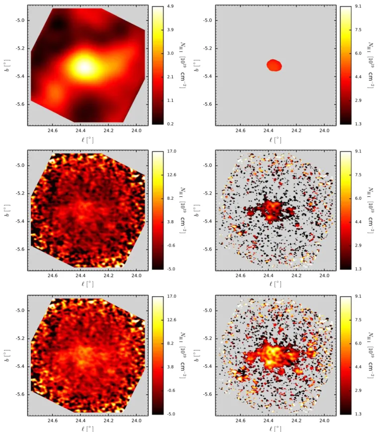
Figure 23. Summary of G24.3−5.3 as described in the caption to Figure11. This cloud, together with G24.7−5.7 and a smaller one that lies between them, form a chain of three clouds connected by diffuse HIemission. G24.3−5.3 has no clear core, but rather several column density peaks of similar values spread over the body of the cloud. Its radial mass proﬁle shows the lack of central concentration. In contrast to G16.0+3.0, which is a core without an envelope, this cloud is an envelope without a core. With a FWHM of 17.4± 1.1 km s−1_{, its line is one of the broadest in the sample.}

(22)

(23)

Figure 26. Summary of G24.7−5.7 as described in the caption to Figure11. A relatively small cloud that together with G24.3−5.3 and a cloud between them forms a chain of three clouds connected spatially and kinematically. Unlike its companion G24.3−5.3, it has a clear core with a narrow line of FWHM = 5.5 km s−1_{, but still}

(24)

Figure 27. HIcolumn density maps for G25.2+4.5, integrated over 64 spectral channels in the interval125.7⩽VLSR⩽166.3km s−1, as described in the caption to

(25)

Figure 29. Summary of G25.2+4.5 as described in the caption to Figure11. The VLA data reveal the considerable complexity of this cloud. There seems to be no single core, but instead many dense regions. The broad line with FWHM= 13.4 km s−1 _{may indicate the blending of several kinematically distinct components within}

the 1′.05 angular resolution of the map, equivalent to 2.35 pc at the adopted distance of the cloud. The cloud has a relatively sharp edge to higher longitudes with diffuse material spreading out to lower longitudes. The relatively broad mass proﬁle and the GBT data suggest that the diffuse components of the cloud may extend well beyond the VLA ﬁeld of view.

(26)

(27)

Figure 32. Summary of G26.9−6.3 as described in the caption to Figure11. A cloud with a sharp boundary toward high latitude and toward the plane, and diffuse material spreading out on the opposite side. More than half of the mass is within 20 pc of the brightest point, but the diffuse material is responsible for the broad mass proﬁle. Its spectrum at peak NHI shows two components with broad and narrow FWHM of 14.5 and 3.0 km s−1, suggestive of a cloud with a two-phase structure. The

(28)

(29)

Figure 35. Summary of G33.4−8.0 as described in the caption to Figure11. This small isolated cloud of ∼160 Me in its dense part is the most distant from the

Galactic plane of any in the sample and has a complex structure. It has many column density maxima spread along a central ridge on the edge closest to the Galactic plane. The spectrum at the highest column density point has two components, one broad and one narrow, suggesting a two-phase thermal structure.

(30)

(31)

Figure 38. Summary of G44.8−7.0 as described in the caption to Figure11. In the spectrum a channel at 74.0 km s−1

is ﬂagged due to an RFI spike. This large, massive cloud extends beyond the primary beam of the VLA. This and the very small cloud G16.0+3.0 are the only clouds whose shape is nearly circular, although the brightest gas is concentrated in numerous small clumps. The spectrum at the NHI peak is asymmetric with a broad wing to higher velocity. This cloud has among the

(32)

Figure 39. Contours for determination of size and mass of clouds based on VLA+GBT (left) and GBT only (right). Top: G16.0+3.0, contour levels

NHI = 2.0 × 10

19

cm−2_{(VLA+GBT) and 5.5 × 10}18_cm−2_{(GBT); bottom: G17.5+2.2, contour levels N}

HI = 5.6 × 10

19

cm−2_{(VLA+GBT) and}

4.4 × 1019cm−2_{(GBT). The dashed lines designate the axes: major (the longest distance between two contour points) and minor (the longest distance between}

contour points in the direction, perpendicular to the minor axis).

Table 6 Measured Cloud Properties

Cloud R z Tb VLSR FWHM Peak NHI (kpc) (pc) (K) (km s−1₎ _{(km s}−1₎ ₍₁₀20_cm−2₎ (1) (2) (3) (4) (5) (6) (7) G16.0+3.0 2.34 +430 12.3± 0.3 143.6± 0.1 4.7± 0.1 1.2 G17.5+2.2 2.56 +310 6.2± 0.3 138.3± 0.4 18.2± 1.0 2.1 G19.5–3.6 2.84 −500 14.6± 0.4 118.8± 0.1 9.9± 0.3 2.9 G22.8+4.3 3.29 +590 4.9± 0.4 135.2± 0.2 5.8± 0.6 1.7 K K 3.2± 0.4 131.7± 0.8 24.3± 2.2 K G24.3–5.3 3.50 −720 2.7± 0.1 125.6± 0.5 17.4± 1.1 0.9 G24.7–5.7 3.55 −770 7.8± 0.3 128.0± 0.1 5.5± 0.2 1.0 G25.2+4.5 3.62 +610 6.3± 0.2 144.5± 0.2 13.4± 0.5 1.6 G26.9–6.3 3.85 −840 13.0± 0.4 120.3± 0.1 3.0± 0.1 2.2 K K 5.2± 0.3 124.1± 0.3 14.5± 0.6 K G33.4–8.0 4.68 −1000 3.5± 0.3 101.9± 0.2 4.3± 0.5 0.8 K K 1.7± 0.3 101.0± 0.8 20.2± 3.1 K G44.8–7.0 5.99 −740 6.8± 0.4 93.4± 0.1 6.1± 0.4 1.7 K K 2.3± 0.3 99.4± 1.1 18.7± 1.5 K

(33)

Figure 40. Contours for determination of size and mass of clouds based on VLA+GBT (left) and GBT only (right). Top: G19.5−3.6, contour levels

NHI = 5.5 × 10

19

cm−2_{(VLA+GBT) and 3.9 × 10}19_cm−2_{(GBT); middle: G22.8+4.3, contour levels N}

HI = 4.1 × 10

19

cm−2_{(VLA+GBT) and}

2.6 × 1019_cm−2_{(GBT); bottom: G25.2+4.5, contour levels N}

HI = 4.3 × 10

(34)

Figure 41. Contours for determination of size and mass of clouds based on VLA+GBT(left) and GBT only (right). Top left: G24.3−5.3 (VLA+GBT), contour at

NHI = 3.1 × 10

19_cm−2_{; bottom left: G24.7−5.7 (VLA+GBT), contour at N}

HI = 2.3 × 10

19_cm−2_{; right: Group of G24.3−5.3 and G24.7−5.7 (GBT), contour at}

NHI = 1.9 × 10

19

cm−2_.

Table 7 Derived Cloud Properties

Cloud R z MHI a Sizea, b á ñn (kpc) (pc) (Me) (pc) (cm−3) (1) (2) (3) (4) (5) (6) G16.0+3.0 2.34± 0.20 +430± 50 45-+1012 16 × 10(0.12) 1.73± 0.20 G17.5+2.2 2.56± 0.23 +310± 40 440 ₁₁₀130 -+ _{43 × 23}_(0.14) _1.10_{± 0.15} G19.5–3.6 2.84± 0.42 −500 ± 100 830-+300370 67 × 28(0.20) 0.80± 0.16 G22.8+4.3 3.29± 0.29 +590± 100 550-+180210 50 × 35(0.18) 0.59± 0.11 G24.3–5.3 3.50± 0.31 −720 ± 140 300-+100130 59 × 29(0.19) 0.33± 0.06 G24.7–5.7 3.55± 0.30 −770 ± 150 290-+100120 60 × 38(0.19) 0.21± 0.04 G25.2+4.5 3.62± 0.34 +610± 130 690-+260320 58 × 48(0.21) 0.37± 0.08 G26.9–6.3 3.85± 0.36 −840 ± 190 600-+240300 66 × 32(0.22) 0.48± 0.11 G33.4–8.0 4.68± 0.41 −1000 ± 280 160-+80100 38 × 28(0.28) 0.36± 0.10 G44.8–7.0 5.99± 0.50 −740 ± 300 840-+550830 62 × 41(0.41) 0.51± 0.21 Notes. a

Clouds’ sizes and masses determined based on contours shown in the left panels of Figures39–42.

b

(35)

Figure 42. Contours for determination of size and mass of a cloud based on VLA+GBT (left) and GBT only (right): Top: G26.9−6.3, contours at

NHI = 5.3 × 10

19

cm−2_{(VLA+GBT) and 1.1 × 10}19_cm−2_{(GBT); middle: G33.4−8.0, contours at N}

HI = 2.5 × 10

19

cm−2_{(VLA+GBT) and 1.2 × 10}19_cm−2_(GBT);

bottom: G44.8−7.0, contours at NHI = 5.5 × 10

(36)

the wind are not well-deﬁned, especially at low latitudes, but the G16.0+3.0 cloud has such distinctive properties as to suggest that its environment is different from that of the other clouds. Within the hot wind the pressure is many times larger than the typical ISM(Bland-Hawthorn & Cohen2003; Carretti et al.2013); this is expected to force clouds into a purely cold phase(Field et al. 1969; Gatto et al.2015). The properties of

G16.0+3.0, with its high density, narrow line width, and compact structure, are consistent with this interpretation. Moreover, G16.0+3.0 is notably smaller then the other clouds, but its size is similar to that of the HIclouds found to be

entrained in the nuclear wind(McClure-Grifﬁths et al. 2013). In contrast, the nearby cloud G17.5+2.2 is nearly indistinguish-able from the other clouds studied here. It might be as close as 135 pc to G16.0+3.0, but is more likely at least 1 kpc away given the uncertainties in our assignment of distances. Neither cloud shows kinematic anomalies suggesting that they have been accelerated by the nuclear wind (McClure-Grifﬁths et al.2013).

We can also compare the properties of our disk-halo clouds with the disk clouds of Stil et al.(2006) observed at similar resolution, but all at z ≈ 0. Only one of their clouds, 59.67–0.39+60 has an analogous morphology and size, with a few times larger mass and average density compared to the clouds of our survey. The properties of all their other clouds are close to our cloud cores, only in some cases displaying a few times larger average density.

These disk-halo HIstructures allow us to study unconfused

interstellar clouds in a variety of locations; this may lead to a better understanding of physical conditions that have hitherto been manifest only in ensemble averages. When the GASKAP survey(Dickey et al.2013) is done, and furthermore when the full SKA is ready, studies like this one will reveal many more such clouds, and the techniques developed here will be useful for understanding their properties.

Table 8

Wide-ﬁeld Cloud Properties Based on GBT Data

Cloud MHI a Sizea, b á ñn (Me) (pc) (cm−3) (1) (2) (3) (4) G16.0+3.0 83-+1921 47 × 43(0.12) 0.07± 0.01 G17.5+2.2 750-+190220 57 × 39(0.14) 0.56± 0.08 G19.5–3.6 1920-+690840 100 × 71(0.20) 0.25± 0.05 G22.8+4.3 1370-+440530 103 × 70(0.18) 0.17± 0.03 G24–5c ₁₁₅₀ 400 480 -+ _{158 × 59}_(0.19) _0.10_{± 0.02} G25.2+4.5 1690-+630780 119 × 75(0.21) 0.16± 0.03 G26.9–6.3 1570-+620780 151 × 85(0.22) 0.08± 0.02 G33.4–8.0 540-+260340 115 × 58(0.28) 0.08± 0.02 G44.8–7.0 2560-+16702530 122 × 85(0.41) 0.19± 0.08 Notes. a

Clouds’ sizes and masses determined based on contours shown in the right panels of Figures39–42.

b

Fractional uncertainties in both dimensions are identical and are given by the value in parentheses.

c

Total for the group of three clouds, containing G24.3−5.3 and G24.7−5.7.

Table 9 Cloud Core Properties

Cloud Contour NHI MHI Size

a nc á ñ Tlimit Tlimit·á ñnc (1020_cm−2₎ _(M e) (pc) (cm−3) (K) (10 3_{K cm}−3₎ (1) (2) (3) (4) (5) (6) (7) G16.0+3.0 0.2 45 ₁₀12 -+ _{16 × 10}_(0.12) _1.7_{± 0.2} ₄₈₀_{± 20} _0.8_{± 0.14} G17.5+2.2 1.5 66-+1719 14 × 6(0.14) 6.7± 0.9 7200± 790 48± 12 G19.5–3.6 2.2 60-+2226 10 × 6(0.20) 10.0± 2.0 2100± 130 21± 6 G22.8+4.3 1.2 57-+1822 11 × 9(0.18) 4.5± 0.8 K K K K K 1.2± 0.2 730± 150 0.9± 0.3 K K K 3.3± 0.6 13000± 2300 42± 15 G23.1+4.3b 0.9 38-+1215 10 × 6(0.18) 6.4± 1.2 K K K K K 2.2± 0.4 590± 200 1.3± 0.7 K K K 4.2± 0.8 7300± 2200 30± 14 G24.3–5.3 0.6 45-+1619 15 × 14(0.19) 1.2± 0.2 6600± 830 7.6± 2.4 G24.7–5.7 0.5 53-+1822 21 × 7(0.19) 2.3± 0.4 660± 50 1.5± 0.4 G25.2+4.5 1.2 57-+2126 15 × 7(0.21) 4.1± 0.9 3900± 290 16± 5 G26.9–6.3 1.3 54-+2127 10 × 7(0.22) 7.2± 1.6 K K K K K 2.5± 0.5 200± 13 0.5± 0.14 K K K 4.7± 1.1 4600± 380 22± 7 G33.4–8.0 0.5 47-+2230 24 × 8(0.28) 1.4± 0.4 K K K K K 0.4± 0.1 400± 90 0.2± 0.1 K K K 1.0± 0.3 8900± 2700 9± 5 G44.8–7.0 1.2 54-+3553 15 × 7(0.41) 3.9± 1.6 K K K K K 1.9± 0.8 810± 110 1.6± 0.8 K K K 2.0± 0.8 7600± 1200 15± 9 Notes. a

Fractional uncertainties in both dimensions are identical and are given by the value in parentheses.

b

A small separate cloud at the high-longitude side of the G22.8+4.3 ﬁeld. First velocity component: Tb= 6.4 ± 0.9 K, VLSR= 129.3 ± 0.3 km s−1, FWHM= 5.2 ±

(37)

Clemens, D. P. 1985,ApJ,295, 422

Dedes, L., & Kalberla, P. W. M. 2010,A&A,509, 60 Dehnen, W., & Binney, J. 1998,MNRAS,294, 429

Dickey, J. M. 2013, in Planets, Stars and Stellar Systems, Vol 5, ed. T. D. Oswalt & G. Gilmore (Dordrecht: Springer Science+Business Media),549

Dickey, J. M., & Lockman, F. J. 1990,ARA&A,28, 215

Dickey, J. M., McClure-Griffiths, N., Gibson, S. J., et al. 2013,PASA,30, 3 Field, G. B., Goldsmith, D. W., & Habing, H. J. 1969,ApJL,155, L149 Ford, H. A., Lockman, F. J., & McClure-Griffiths, N. M. 2010,ApJ,722, 367 Ford, H. A., McClure-Griffiths, N. M., Lockman, F. J., et al. 2008, ApJ,

688, 290

Gatto, A., Walch, S., mac Low, M.-M., et al. 2015,MNRAS,449, 1057 Heiles, C., & Troland, T. H. 2003,ApJ,586, 1067

Heiles, C., & Troland, T. H. 2005,ApJ,624, 773 Hobbs, L. M. 1978,ApJ,222, 491

Jenkins, E. B. 2012, in EAS Pub. Ser. 56, The Role of the Disc-Halo Interaction in Galaxy Evolution: Outﬂows versus Infall?, ed. M. A. de Avillez(Les Ulis: EDP Sciences),31

Jenkins, E. B., & Tripp, T. M. 2011,ApJ,734, 65 Kalberla, P. M. W., & Kerp, J. 2009,ARA&A,47, 27 Kerr, F. J., & Lynden-Bell, D. 1986,MNRAS,221, 1023 Koyama, H., & Ostriker, E. C. 2009,ApJ,693, 1346

Kulkarni, S. R., & Heiles, C. 1987, in Interstellar Processes, ed. D. Hollenbach & H. Thronson(Dordrecht: Reidel), 87

Lallement, R., Welsh, B. Y., Vergely, J. L., Crifo, F., & Sfeir, D. 2003,A&A, 411, 447

Lazarian, A., & Pogosyan, D. 2000,ApJ,537, 720 Lockman, F. J. 1984,ApJ,283, 90

Lockman, F. J. 2002,ApJL,580, L47

Rathborne, J. M., Jackson, J. M., Chambers, E. T., et al. 2010,ApJ, 715, 310

Redﬁeld, S., & Linsky, J. L. 2008,ApJ,673, 283

Sault, R. J., & Killeen, N. 2011, 26 May 2011, Miriad Users Guide, Australia Telescope National Facility, ftp://ftp.atnf.csiro.au/pub/software/miriad/ userguide_US.ps.bz2

Sault, R. J., Teuben, P. J., & Wright, M. C. H. 1995, in ASP Conf. Ser. 77, Astronomical Data Analysis Software and Systems IV, ed. R. Shaw, H. E. Payne & J. J. E. Hayes(San Francisco, CA: ASP),433

Saury, E., Miville-Deschênes, M.-A., Hennebelle, P., Audit, E., & Schmidt, W. 2014,A&A,567, A16

Shane, W. W. 1967, in IAU Symp. 31, Radio Astronomy and the Galactic System ed. H. van Woerden(London: Academic),177

Simonson, S. C. 1971, A&A,12, 136

Stanimirović, S. 1999, PhD thesis, Univ. Western Sydney Nepean Stanimirović, S., Putman, M., Heiles, C., et al. 2006,ApJ,653, 1210 Stanimirović, S., Staveley-Smith, L., Dickey, J. M., Sault, R. J., &

Snowden, S. L. 1999,MNRAS,302, 417

Stil, J. M., Lockman, F. J., Taylor, A. R., et al. 2006,ApJ,637, 366 Strasser, S. T., Dickey, J. M., Taylor, A. R., et al. 2007,AJ,134, 2252 Su, M., Slatyer, T. R., & Finkbeiner, D. P. 2010,ApJ,724, 1044

Vázquez-Semadeni, E. 2012, in EAS Pub. Ser. 56, The Role of the Disc-Halo Interaction in Galaxy Evolution: Outﬂows versus Infall?, ed. M. A. de Avillez(Les Ulis: EDP Sciences),39

Welsh, B. Y., Lallement, R., Vergely, J.-L., & Raimond, S. 2010, A&A, 510, AA54

Wolﬁre, M. G., Hollenbach, D., McKee, C. F., Tielens, A. G. G. M., & Bakes, E. L. O. 1995a,ApJ,443, 152

Wolﬁre, M. G., McKee, C. F., Hollenbach, D., & Tielens, A. G. G. M. 1995b,