An automation approach to guiding an air vehicle through an obstacle field

An Automaton Approach to Guiding an Air Vehicle Through an Obstacle Field

by

Rebecca Jane Dailey B.S., Mechanical Engineering

Massachusetts Institute of Technology, 1998

Submitted to the Department of Aeronautics and Astronautics in Partial Fulfillment of the Requirements for the Degree of

Master of Science in Aeronautics and Astronautics at the

Massachusetts Institute of Technology February 2002

@ 2002 Rebecca J. Dailey

All rights reserved.

AEROI

The author hereby grants to MIT permission to reproduce and to

distribute publicly paper and electronic copies of this thesis document in whole or in part.

In .. .A

Signature of Author

~'- /

/1 _{,A .}

...

Department of Aeronautics and Astronautics

) A October 1, 2001

C ertified by... . .. ... . ...

James D. Paduano Principal Research Engineer 7 hesis

Supervjsor

Accepted by... ... .. ....

Wallace E. Vander Velde Professor of Aeronautics and Astronautics Chair, Committee on Graduate Students

ASSACHUSETTS 1ISTITUTt

OF TECHNOOGY

AUG

1 3 2002

An Automaton Approach to Guiding an Air Vehicle Through an Obstacle Field

by

Rebecca Jane Dailey

Submitted to the Department of Aeronautics and Astronautics on October 1, 2001 in Partial Fulfillment of the

Requirements for the Degree of Master of Science in Aeronautics and Astronautics

ABSTRACT

This thesis addresses the problem of guiding an air vehicle through an unknown obstacle laden environment to a specified destination, while maintaining a low altitude. Potential applications for recently developed micro air vehicles (MAVs) are described, illustrating the need for autonomy in such vehicles. A scenario is presented in which an MAV is deployed from a parent vehicle and instructed to fly autonomously to a certain location, without colliding with any obstacles. The MAV must have a guidance algorithm to determine its trajectory, as well as an inner loop controller to actually fly this trajectory.

A finite state automaton architecture for the guidance algorithm is proposed. A set of

states and logical transitions between them is defined and presented. A series of simulations through several environments is used to test the proposed approach. The results of these tests are presented and analyzed, and the failure modes are explained. The results help to determine the requirements on the MAV's sensor system, and the minimum amount of information and processing required to accomplish the mission. Finally, conclusions are drawn regarding the inherent properties of finite state automata, and future work is recommended to improve upon the automaton approach to obstacle avoidance developed here.

Thesis Supervisor: James D. Paduano Title: Principal Research Engineer

Table of Contents 1.0 Introduction

1.1 Overview ... 5

1.2 Potential Applications... 5

1.3 Related Research ... 6

2.0 Problem Statement and Preliminary Assumptions 2.1 Problem Statement...8

2.2 Assum ptions on Environment ... 8

2.3 Assum ptions on M AV ... 8

2.4 Desired Results... 9

3.0 Proposed Approach 3.1 Basic Architecture of Guidance Algorithm ... 10

3.2 Overview of Logic ... 10

3.3 State Definitions ... 13

3.4 State Transitions ... 14

3.5 Sum m ary of Proposed Approach... 22

4.0 Flight Dynamics 4.1 Aircraft Sim ulation and Analysis ... 23

4.2 Optim al Velocity ... 28

5.0 Results 5.1 Test Environm ents ... 30

5.2 Failure M odes and Negative Effects... 35

5.3 Robustness... 41

6.0 Conclusions and Future Work 6.1 Sum m ary of Architecture... 42

6.2 Conclusions ... 42

7.0 References ... 44

Appendices Appendix A .1 - M AV Specifications ... 45

Appendix A .2 - Autom aton Design Parameters... 46

List of Figures

Figure 3.1.1 - System B lock D iagram ... 10

Figure 3.2.1 - Sam ple Polygon ... 11

Figure 3.2.2 - Model of a Building, Segmented into 8 Obstacles ... 12

Figure 3.2.3 - Example of Inside Corner ... 13

Figure 3.3.1 - State Transition Diagram ... 13

Figure 3.4.1 - Logic flow for state STRAIGHT ... 15

Figure 3.4.2 - Logic flow for state TARGETHOLD ... 16

Figure 3.4.3 - Logic flow for state MAXTURN ... 17

Figure 3.4.4 - Logic flow for state HOLDALONGOBS ... 18

Figure 3.4.5 - Logic flow for state HEADTOCORNER... 18

Figure 3.4.6 - MAV Trajectory through a Single Building Environment ... 21

Figure 4.1.1 - Block Diagram of MAV Flight Control System ... 23

Figure 4.1.2 - Frequency Response and Root Locus for Flight Path Angle (Gamma)...24

Figure 4.1.3 - Frequency Response and Root Locus for Altitude...25

Figure 4.1.4 - Frequency Response and Root Locus for Velocity ... 26

Figure 4.1.5 - Frequency Response and Root Locus for Yaw Rate ... 27

Figure 4.2.1 - Turning Capabilities of the MAV... 29

Figure 5.1.1 - Test Environm ent 1... 30

Figure 5.1.2 - Trajectories through Test Environment 1 ... 31

Figure 5.1.3 - Test Environm ent 2... 32

Figure 5.1.4 - Trajectories through Test Environment 2 ... 33

Figures 5.1.5a and 5.1.5b - Sample Trajectories through Harvard Square...34

Figure 5.2.1 - Example of Trajectory Loop from Environment 2...35

Figure 5.2.2a - Example of Obstacle Collision from Environment 1...36

Figure 5.2.2b - Close-Up of Obstacle Collision from Environment 1... 37

Figure 5.2.3a - Example of Missed Outside Corner from Environment 1... 39

Figure 5.2.3b - Close-Up of Missed Outside Corner from Environment 1 ... 40

Figure A.3.1 - Simulink Diagram of MAV Automaton System...48

Figure A.3.2 - Stateflow Diagram of Guidance Algorithm ... 49

List of Tables

Table A. 1.1 - M AV Specifications... 45

Table A.2.1 - Automaton Design Parameters ... 46

1.0 Introduction

Recent advances in technology have given rise to the development of Micro Air Vehicles, or MAVs. These tiny airplanes, less than 12 inches in wingspan, are being considered for a wide range of applications, in both the military and civilian realms. In all of these applications, control is one of the primary challenges. It is desirable to make the MAV as autonomous as possible, so that it can be given a task and sent on its way, with little to no

additional information or processing required from an external source. This paper proposes an automaton approach to this scenario, which will safely guide an MAV through an obstacle field to some given destination.

1.2 Potential Applications

With the development of miniature sensors, many possible uses for MAVs have recently been suggested. Equipped with a camera, MAVs could be used in a combat setting to perform over-the-horizon reconnaissance missions, or photograph enemy territory. They could also perform military reconnaissance in an urban environment. They could be used to deliver sensors to remote locations, detect biological or chemical agents, or locate

landmines. In a more civilian context, they could search for survivors after an earthquake or fire. They could even be used to monitor weather or traffic patterns. Due to the limited range of such small aircraft, a multi-vehicle approach is being considered. In this approach, a larger Unmanned Air Vehicle (UAV) carries the MAV to an area near where it must perform its mission. It then deploys the MAV, which can fly at a lower altitude and more easily navigate through an obstacle-laden environment than its parent vehicle. Once the mission is complete, the MAV could either land at some specified destination, or could rendezvous with a larger UAV to return home.

In this context, there are several issues to consider. The parent UAV may have its own mission to carry out, or may be managing multiple MAVs simultaneously. Therefore, it is desirable for each MAV to be able to operate autonomously, and rely on the parent vehicle as little as possible. Ideally, the parent would provide the MAV with basic information about its mission, such as the destination, and then send it on its way. The parent is then free to focus on other tasks, assuming that the MAV's own controllers will be able to successfully complete the mission. This is analogous to the way an outer control loop treats an inner control loop in a typical feedback control architecture. For example, an outer loop controller may generate a trajectory for a certain vehicle to follow. It inputs this trajectory to the inner loop, which does what it needs to do to make the vehicle follow the assigned trajectory. The outer loop controller is not involved in this process, as long as the inner loop is designed properly. This paper proposes an approach that enables the MAV guidance algorithm to appear to the parent vehicle as simple and independent as an inner loop appears to an outer loop.

A common practice to design a good inner loop controller is to use feedback. Feedback

provides stability and minimizes the effects of unwanted disturbances. Optimal system responses can be obtained from a properly designed state feedback controller. In the

above trajectory-following example, the vehicle's position is typically fed back and subtracted from the input (the given trajectory), and then this error is applied to the actuators with some appropriate gain to force the vehicle to the desired position. This practice is both stable and robust, and will successfully drive the vehicle to the desired trajectory. In this thesis, we investigate the hypothesis that there is a method analogous to feedback that can enable an obstacle avoidance algorithm to be stable and to achieve

some of the robustness properties of feedback-based control loops.

To test this hypothesis, we propose a finite state automaton architecture for the guidance algorithm. In other words, the algorithm consists of a set of discrete states, such as "straight flight" or "maximum turn." It receives information from the sensors and

communication system about the outside world, and combines this with measurements of the vehicle's own position and heading. It then uses a set of logical rules to determine in which state it should be. The state of the guidance algorithm specifies a command or set of commands that are to be issued to the inner loop controller. State transition tests are performed every cycle, using the latest information available. In this way, the algorithm is able to react to its environment and adjust the vehicle's trajectory accordingly, while driving the vehicle to the given destination.

We further postulate that to achieve properties analogous to those of feedback loops, the method should have the following three properties:

e Immediate or nearly immediate use of sensed information about the obstacle field.

This could also be termed feedback.

" A simple formulation, based on intuitive notions of the physical relationships

governing the obstacle avoidance problem. Simplicity of the method is important for use on an MAV, as the vehicle's small size might greatly limit its onboard memory and processing capabilities.

e Primary reliance on current state, rather than past or predicted state. This implies

that the behavior of the vehicle in a particular state will be consistent and straightforward.

This thesis deals primarily with applications in which an MAV must travel through an obstacle-laden environment, such as a city, to reach some specified destination.

Therefore, the primary function of the MAV's guidance algorithm is obstacle avoidance. In these applications, we will also assume that the MAV is required to maintain a low altitude, so that simply pulling up and flying over a building is not practical. The obstacle avoidance algorithms employed must be simple, stable, and not heavily

dependent on external information. Other researchers have investigated similar obstacle avoidance problems, particularly in the field of robotics. Their findings will now be described.

1.3 Related Research

The problem of obstacle avoidance is not a new one, and many researchers have

with generating the shortest path for a robot to follow through a field of circular obstacles to reach a goal [1,2]. Shiller makes use of the return function, which he defines as the length of the shortest path from any initial point to the goal. To help in evaluating the return function, Shiller also defines "obstacle shadows," which can be thought of as shadows cast by obstacles when a point light source is located at the goal. If the initial point does not lie in the shadow of any obstacles, then obviously the shortest path is simply a straight line from the point to the goal. If the initial point does lie in the shadow of an obstacle, then the shortest path consists of "a straight line, a constrained arc that follows the obstacle boundary, then a straight line to the goal." Obstacle-free paths are generated by following the negative gradient of the return function. In environments with multiple obstacles, only the nearest obstacle is processed. Cases in which an obstacle is encountered while another one is being processed are treated separately. Shiller's results show that by optimally avoiding one obstacle at a time, a near-optimal path through the entire environment is generated. This algorithm works well, and can readily be adapted for our purposes.

H. Choset has also investigated the problem of sensor-based planning [3,4]. In his work, the goal is not to reach some location, but to exhaustively explore some unknown

environment. This is done using a type of roadmap called a Voronoi Diagram. This diagram represents the set of all points in an obstacle field equidistant from two or more obstacles. Once a robot has traced out the Voronoi Diagram, then everything about the environment is known. Creating this diagram is not important for our purposes, since the goal here is to reach a destination. However, the ideas encapsulated in the Voronoi Diagram give important information about the environment, as will be demonstrated in section 3.2.

E. Frazzoli has also performed research in the area of motion planning [5,6]. He has developed an algorithm that he terms a maneuver automaton. This automaton uses

"'maneuvers" to move between "trim trajectories," thereby creating an obstacle-free path through an environment. This research validates the proposal that continuous systems can be controlled using logic of a discrete nature. However, Frazzoli's work deals only with vehicles such as helicopters or robots, which can stop anywhere, and turn on a point. Fixed-wing aircraft must remain in motion at all times and have limited turning

capabilities. This must be taken into account when developing the guidance algorithm. Finally, much research has been done in the context of fully known environments, where the goal is to generate an optimal path. The focus of this thesis is unpredictable

situations, where the question of optimality becomes irrelevant. It does not make sense to go through laborious computations to determine a trajectory that minimizes some cost, and then quickly discover that that trajectory is no longer feasible, and have to start all over again. It is more important to focus on reaching the destination. By making this the ultimate goal, the resulting trajectory may or may not be optimal, but the mission will be successful.

2.0 Problem Statement and Preliminary Assumptions

The goal of this research is to develop an algorithm that will guide an air vehicle from some initial location to some specified destination, while avoiding any obstacles that exist in the environment, and maintaining a low altitude. This algorithm should be simple, requiring as little information and processing as possible. We will use a

nonlinear 6 degree-of-freedom simulation of an MAV, adapted from Miotto and Paduano

[7], to perform this study. The final result will be a guidance algorithm, to be used as a

real-time path planner, driving the MAV to the destination while avoiding obstacles. The secondary goals of this study are to determine the requirements on the vehicle's sensor system, and to qualitatively investigate the robustness properties of reactive automaton-based algorithms.

No a priori information about the environment is provided to the guidance algorithm. However, some assumptions about both the environment and the MAV's capabilities must be made. These assumptions will now be described.

2.2 Assumptions on Environment

The environment will be modeled after a city, where the buildings are the obstacles. The MAV will be required to maintain a low altitude, well below the building roofs, but high enough so that trees and utility poles do not pose a danger. The buildings will be polygonal in shape (from an aerial perspective). The MAV will be able to fly in the free space between the buildings. This space would most likely be above the city streets, and so will be scaled accordingly. The destination, or "target" may be slowly moving, but its location is known to the MAV at all times. The target is assumed to be in the same free space as the MAV, with no obstacles within a sufficient radius from it.

In addition, we have decided to treat the problem as a planar one. The requirement of maintaining a low altitude prohibits the MAV from being able to use altitude as a degree of freedom to aid in avoiding obstacles. Therefore, the guidance algorithm will not command altitude changes. It will be the responsibility of the inner loop controller to account for changes in altitude due to turns. All obstacle avoidance and target acquisition logic will be based in a 2-dimensional frame; namely, north and east.

2.3 Assumptions on the MAV

The MAV will know its own location and heading at all times. It will also be equipped with both communication and sensor equipment. The communication system will provide the MAV with target positional data. This information will be updated at a frequency of at least 1 Hz. The MAV will rely on the sensor system for obstacle

detection. Further details and requirements on this sensor system are to be determined by the obstacle avoidance logic implementation, and will be described in section 3.2. The MAV will also have adequate computer processing power so that it can react

delays are expected to be on the order of tens of milliseconds, so that our results will still be applicable. The MAV's inner loop controller takes the commands generated by the guidance algorithm and generates actuator commands from them, thereby guiding the MAV to the desired trajectory.

2.4 Desired Results

The main result of this research will be the design for a guidance algorithm that will accomplish the goal of guiding an air vehicle through an obstacle field to a specified destination. The requirements for the sensor system on the vehicle will be determined, as well as the minimum amount of information and processing required. A simulation of the proposed architecture will be developed and run, so that the system performance can be analyzed. Finally, some qualitative conclusions will be made regarding the robustness properties of reactive automaton-based algorithms.

3.0 Proposed Approach

3.1 Basic Architecture of Guidance Algorithm

From the problem statement, it can be seen that the MAV must be a reactive system, since it is operating on limited information about its environment. The goal of the system can actually be broken into two separate missions: 1) reach the target; and 2) avoid all obstacles. We propose that the simplest architecture for achieving the missions in this context of limited information is a finite state automaton. This method is consistent with the objective of creating a simple, stable, independent guidance algorithm, and analogies can be made to the feedback approach widely used in inner loop controller design. The following block diagram represents our view of how the guidance algorithm interacts with the outside world and with the aircraft itself.

.ouncto (Finite EnviroteSta

obstacle

inform-Sensor ation

System Gurae ca ted flight pat

target Gritinh _o__and sompen-

Aircrafto--beAde d info liti s

'ommunication ation (Finite State sa oss rate and

System atif the Automaton) position

l sensors

leada ing fe stability and command augmentation loops

position

Figure 3.1.1 - System Block Diagram.

The basic ideas behind the definitions of states and state transitions in the automaton will be described in the following section.

3.2 Overview of Logic

The logic to achieve the goal will make us te etwo main erferences described in

section 1.3; namely, Shiller's "obstacle shadows" and Choset's "Voronoi Diagrams."

Shiller states that if the initial point is not in the shadow of any obstacles, then the best trajectory is a straight line from that point to thareto Ie einitial point does le in the

shadow of some obstacle, then the best trajectory is one which runs parallel to the

obstacle boundary until breaking free of the shadow, and then a straight line to the target. Although Shiller's work deals with circular obstacles, the same logic can be applied to line segments.

Because the MAV's sensor system has a finite range, entire buildings will not be detected at once. Rather, small regions will come into view as the MAV approaches them. In order to model this, we divided obstacle boundaries into line segments of various lengths.

A set of these segments forms a continuous, non-overlapping closed contour that

represents the outside of a building. In our terminology, the word "obstacle" will refer to one of these individual line segments. Once any portion of an obstacle enters into the sensor system's range, the obstacle is considered detected. This is consistent with Choset's idea that "the distance between a point and an obstacle is the shortest distance between the point and all points in the obstacle." The location of a detected obstacle's

endpoints are known, and the headings of the obstacles on either side of it are also known. The reason this information is important will be described further in a subsequent paragraph.

Clearly, there must be a sensor that can detect obstacles directly in front of the MAV. When such an obstacle is detected, the MAV is commanded to turn to a heading parallel to the obstacle's heading, and fly in this direction until the obstacle no longer poses a threat. Obviously, there are two such headings parallel to a line segment, which differ by

180'. With limited information, it is impossible to determine which heading is the "best"

from the perspective of the ultimate goal of reaching the target. However, collision avoidance is the overriding requirement, even if such avoidance compromises the

optimality of the path to the target. Clearly, the MAV should turn to the heading which is closest to its current heading. This prevents the MAV from attempting a very large heading change (or even a circle) that it may not be able to complete without colliding with the obstacle.

We have employed Shiller's logic to help satisfy the goal of reaching the target. The MAV must have a sensor that can be oriented in the direction of the target at all times. This sensor will detect obstacles that lie in the MAV's line of sight to the target. In other words, it will detect if the MAV lies in the shadow of an obstacle. If so, then as above, the MAV is commanded to turn to the closest heading parallel to the obstacle's heading, and fly in this direction until it is no longer in the shadow of this obstacle.

There are several deviations from this basic logic structure, primarily relating to corners of buildings. Corners can be categorized into outside corners and inside corners, according to the following figure:

0

0

Figure 3.2.1 - Sample Polygon.

In this figure, corners 1,2,3,4, and 6 are outside corners, while corner 5 is an inside

be discriminated, both during sensing and in the guidance algorithm. We have developed a concept which we call "Voronoi vectors" as a convenient way to handle this. Based on the fundamentals of Voronoi Diagrams, a vector can be drawn from every obstacle endpoint in a direction that is equidistant from the two obstacles that meet at that point, and pointed away from the interior of the building. This vector is referred to as the Voronoi vector. The following figure illustrates this concept:

Figure 3.2.2 - Model of a Building, Segmented into 8 Obstacles. The corresponding Voronoi vectors are shown.

As mentioned above, when the sensor system detects an obstacle, it must also detect the heading of the two obstacles adjacent to the current obstacle. From this information, the Voronoi vector direction from each endpoint of the current obstacle can be calculated. Therefore, every obstacle has six pieces of information associated with it: the

(north,east) coordinates of both endpoints, and the Voronoi vector directions for both endpoints.

Note: In the simulation, the obstacle information is kept in a database. Each obstacle is catalogued separately, so the coordinates and vector associated with each endpoint are

actually listed twice, once for each obstacle that emanates from that endpoint. From the direction of the Voronoi vector, outside corners and inside corners can be identified. If an obstacle in the MAV's line of sight to the target has an outside corner, then it is better to command the MAV towards this corner instead of parallel to the obstacle. This helps drive the MAV around the corner and closer to the target. If an obstacle in the MAV's direct path has an inside corner, special care must be taken to prevent the MAV from having to execute a very sharp turn and/or pass too close to the adjacent obstacle. If the MAV is able to turn parallel to the obstacle in the direction away from the inside corner without requiring a change in heading of more than 1350, then this should be done. Otherwise, the MAV should turn parallel to the obstacle in the direction closest to its current heading; i.e., execute a standard avoidance maneuver. It will then detect the adjacent obstacle and react accordingly. The following figure illustrates this logic.

A

B

2

1

Figure 3.2.3 - Example of Inside Corner. The heavy lines, labeled A and B, represent 2 obstacles that form an inside corner. The arrows show 2 trajectories approach this corner, both of which will intersect with obstacle B. The inside corner logic dictates that the vehicle following trajectory 1 should turn right, to avoid a collision with obstacle A. However, since trajectory 2 is approaching obstacle B at a much more shallow angle, the logic dictates that the vehicle following

trajectory 2 should turn left, and fly parallel to obstacle B towards obstacle A. After making this left turn, obstacle A will be detected, and the vehicle will turn left again.

Only one obstacle at a time is considered, as in Shiller's work. If more than one obstacle is detected, only the closest one is processed.

3.3 State Definitions

The next figure shows the proposed state transition diagram, which follows from the logic described above. A description of the states follows. The next section will describe the state transitions in detail.

STRAIGHT

TARGETHOLD

Turn gently to orient parallel to obstacle

HOLDALONGOB _HEADTOCORNER

MAXTURN

3.3.1 STRAIGHT

In this state, the MAV is commanded to fly straight along its current heading.

3.3.2 TARGETHOLD

This state calculates the line of sight from the MAV to the target, then uses proportional feedback to command the MAV to turn to this heading. A limit is imposed on the turning rate to keep the turns gentle.

3.3.3 MAXTURN

This state takes an obstacle as an input. It commands the MAV to turn parallel to this obstacle, using the maximum turn rate that the MAV can handle.

3.3.4 HOLDALONGOBS

This state also takes an obstacle as an input. It commands the MAV to turn parallel to this obstacle, using proportional feedback with a limit as in the TARGETHOLD state. 3.3.5 HEADTOCORNER

This state takes an obstacle with an outside corner as an input. It commands the MAV to turn toward a point located a specified distance out from the outside corner, along the Voronoi vector. Proportional feedback with a limit is employed, as in the

TARGETHOLD state. Note that this process requires knowledge of the MAV's current position.

With these five states, the logic described above can be implemented. The state transitions will now be described in detail.

3.4 State Transitions

The state transitions are the key to encapsulating the proposed obstacle avoidance and target acquisition logic. They are best illustrated using logic flowcharts. The next five figures show the logic flow and subsequent possible transitions from each of the five states. The transitions are then described in detail.

yes

no

Does obstacle in

LOS to target have

an outside corner in the direction the

MAV is headed?

no

HEADTOCORNER input: obstacle in LOS to target

Figure 3.4.1 - Logic flow for state STRAIGHT.

no

yes

no

no

Does obstacle in

LOS to target have

an outside corner in the direction the

MAV is headed?

no

HEADTOCORNER input: obstacle in LOS to target

Figure 3.4.2 - Logic flow for state TARGETHOLD.

no

no

HEADTOCORNER

input: given obstacle

Is a heading change of

more than 1350 required for

the MAV to be parallel to the given obstacle, headed

away from the inside corner?

HOLDALONGOBS

input: given obstacle

Figure 3.4.3 - Logic flow for state MAXTURN. yes

yes

no

Figure 3.4.4 - Logic flow for state HOLDALONGOBS.

Figure 3.4.5 - Logic flow for state HEADTOCORNER. no

The individual transitions between states will now be described. For clarity, we will define a LOS obstacle to be an obstacle in the MAV's line of sight to the target. 3.4.1 STRAIGHT to TARGETHOLD

If the MAV is traveling straight but not in the direction of the target, and no obstacles are

detected from either sensor, then a transition to TARGETHOLD should be executed to gently turn toward the target.

3.4.2 STRAIGHT to MAXTURN

If the MAV is flying straight and an obstacle is detected in its direct path, then it should

transition to MAXTURN to avoid this obstacle. Or, if the MAV is flying straight and a

LOS obstacle is detected that is not parallel to the current heading of the MAV, then this

transition should take place, unless this obstacle lies entirely behind the MAV. 3.4.3 STRAIGHT to HEADTOCORNER

If the MAV is flying parallel to a wall that is in its line of sight to the target, and an

outside corner is detected in the direction the MAV is traveling, then a transition should be made to the HEADTOCORNER state to drive the MAV around the outside corner and closer to the target.

3.4.4 TARGETHOLD to STRAIGHT

This transition is made when the MAV achieves the desired heading toward the target. Or, if in the process of turning toward the target a LOS obstacle is detected that is parallel to the current heading of the MAV, then the MAV should fly STRAIGHT along this obstacle, unless this obstacle has an outside corner in the direction the MAV is traveling. 3.4.5 TARGETHOLD to MAXTURN

If the MAV is turning toward the target and an obstacle is detected in its direct path, then

it should transition to MAXTURN to avoid this obstacle. Or, if the MAV is turning toward the target and a LOS obstacle is detected that is not parallel to the current heading of the MAV, then this transition should take place, unless the obstacle lies entirely behind the MAV.

3.4.6 TARGETHOLD to HEADTOCORNER

If in the process of turning toward the target a LOS obstacle is detected that is parallel to

the current heading of the MAV, and this obstacle has an outside corner in the direction the MAV is traveling, then this transition should be made to drive the MAV around the outside corner and closer to the target.

3.4.7 MAXTURN to HOLDALONGOBS

If the MAV is executing a sharp turn to avoid an obstacle, and the MAV is nearly parallel

to this obstacle (within a substantial tolerance), then a transition to

HOLDALONGOBS should be made, so that a more gentle turn will be executed.

3.4.8 MAXTURN to HEADTOCORNER

If the MAV has been directed to execute a sharp turn to avoid a LOS obstacle, and this

obstacle has an outside corner in the direction the MAV is headed, this transition should be made to drive the MAV around the outside corner and closer to the target.

3.4.9 HOLDALONGOBS to STRAIGHT

This transition is made when the MAV achieves the desired heading, parallel to the given obstacle.

3.4.10 HOLDALONGOBS to MAXTURN

If the MAV is gently turning parallel to an obstacle and another obstacle is detected in its

direct path, then a transition to MAXTURN is made to avoid the new obstacle. 3.4.11 HEADTOCORNER to TARGETHOLD

If the MAV is heading for an outside corner of an obstacle, this transition is made once

the obstacle is no longer in the MAV's line of sight to the target. 3.4.12 Illustrative Example

To better illustrate the state transition logic, here is an example involving a very simple environment.

120 -0 0 C z 100-0 01 a. 80 _F 60- 40- 20-0 -100 -50 0 50 100 Position East (m)

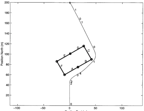
Figure 3.4.6 - MAV Trajectory through a Single Building Environment.

First, a brief note about the coordinate system: Coordinates are stated as (East, North). Distances are given in meters, and headings are given in degrees. A 0' heading is due north, with clockwise being the positive direction. Consequently, a 900 heading would be due east, and a -135' heading would be southwest.

In Figure 3.4.6, the MAV begins at location (0,0), on a 0' heading. It must reach a stationary target at (0,200), denoted on the plot with a star (*). There is one rectangular building in the environment. For modeling purposes, it has been broken into six

segments of 30m in length, labeled A through F. The MAV can detect any of these obstacles within a range of 20m. The numbers along the trajectory indicate state transitions, as listed in the following table:

Number

State

0 STRAIGHT

1 TARGET HOLD

2 MAXTURN

3 HOLD ALONG OBS

4 HEAD TO CORNER

The MAV always begins in state STRAIGHT. Since it is initially headed for the target, it remains in this state until an obstacle is encountered. The first obstacle to be detected is obstacle A, that is both in the line of sight to the target, and in the direct path of the MAV. Therefore, a transition to state MAXTURN is performed, to avoid this obstacle. Obstacle A does not have any outside or inside corners in the direction the MAV is headed (towards obstacle B). Therefore, MAXTURN will generate the maximum turn rate command that the MAV is capable of handling. The sign of this command, which corresponds to a left or right turn, will be based on whichever direction will orient the MAV parallel to obstacle A with minimal heading change. Here, this means a right-hand turn. Once the MAV is somewhat parallel to obstacle A (within a tolerance of 40'), a transition to state HOLDALONGOBS is made. In this state, gentler, proportional turn rate commands are issued to orient the MAV parallel to obstacle A. Here, this desired heading is 600. Since no other obstacles are encountered in the meantime, the MAV stays in state HOLDALONGOBS until it is parallel to obstacle A (within a tolerance of

1.7'). Then the MAV transitions to state STRAIGHT, since it has taken the steps

necessary to avoid obstacle A.

Now, obstacle A is still in the MAV's line of sight to the target. However, since the MAV is already parallel to it, and there is nothing in its direct path, it remains in state STRAIGHT until it crosses over into the shadow of obstacle B. Since obstacle B has an outside corner in the direction the MAV is headed (towards obstacle C), a transition to state HEADTOCORNER is made. In this state, proportional turn rate commands are issued to orient the MAV on a heading towards an aimpoint. This aimpoint is located at 5m out from the corner formed by obstacles B and C, along the Voronoi vector (the vector which points away from the interior of the building, and bisects the angle formed

by obstacles B and C). The MAV will stay in this state and head for the aimpoint until

obstacle B is no longer in its line of sight to the target. Once this occurs, a transition to state TARGETHOLD is performed. In this state, proportional commands are issued to point the MAV towards the target. Since no other obstacles are detected in the meantime, the MAV remains in this state until it reaches the desired heading (within a tolerance of

1.1 ). It then transitions to state STRAIGHT and continues flying towards the target. No

other obstacles are detected. Some minor corrections are made along the final stretch, and then the MAV successfully reaches the target. This completes the mission.

3.5 Summary of Proposed Approach

The architecture for the MAV's guidance algorithm will be a finite state automaton, with the five states and transitions between them described above. The algorithm will take as inputs the position and heading of the MAV and the location of the target. The MAV will need two sensors, one that will detect obstacles in the MAV's direct path, and one that will detect obstacles in the MAV's line of sight to the target. The guidance

algorithm will output a yaw rate command to be issued to the inner loop controller. No other commands are needed. With this architecture, the algorithm will accomplish the mission of guiding the MAV to the target without colliding with any obstacles.

4.0 Flight Dynamics

4.1 Aircraft Simulation and Analysis

The simulation used for testing the proposed obstacle avoidance logic is based upon a nonlinear flight simulator for Matlab and Simulink, developed by Piero Miotto and James Paduano. A complete description of it can be found in [7]. In this simulation,

aerodynamic forces and moments are computed based on calculated aerodynamic

derivatives for the MIT MAV, as well as nonlinear aerodynamic effects (i.e., wing stall). This modeling work was performed by Prof. Mark Drela. (See Appendix A. 1 for a complete listing of the MAV specifications, including dimensions and stability

derivatives.) We made several modifications to this simulation, to allow for stabilization of altitude. A frequency analysis was then performed on the entire aircraft flight control system.

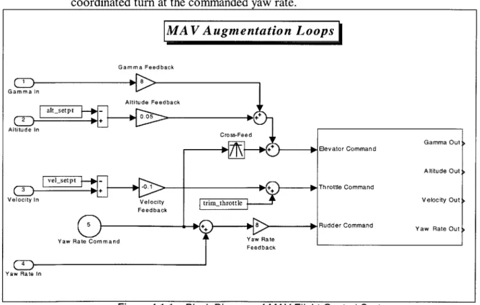
The aircraft model used here is a 3-input, 4-output system, as shown in the following figure. The available inputs are elevator, throttle, and rudder. The system outputs are flight path angle, altitude, velocity, and yaw rate. The system consists of three parts:

e Altitude hold loop, with proportional and derivative (flight path angle) feedback. " Crude velocity hold loop. This loop was not part of the design work done for this

thesis. It is adequate for our needs, and is presented here for completeness.

e Yaw rate command loop, that uses rudder-to-roll attitude coupling to achieve turn

coordination. Elevator deflection is instantaneously set to the trim value for a coordinated turn at the commanded yaw rate.

Figure 4.1.1 - Block Diagram of MAV Flight Control System. MAV Augmentation Loops

Gamma Feedback

The following sections describe the open- and closed-loop frequency response and root locus of each channel, with a close-up of the root locus around the origin. The open-loop response is represented with a dotted line, and open-loop poles and zeros are represented

by x's and o's, respectively. The closed-loop response is represented by a solid line, and

the closed loop poles are designated with stars along the root locus.

4.1.1 Flight Path Angle (y) Feedback

Open Loop and Closed Loop Frequency Response for Gamma

30 20 10 0 -10 -20 -30 -40 -50 10 50 0 -50 -100 -150 -200 -250 100 Frequency, rad/sec ROOT LOCUS 35 30 , 25 20 E 10 5 -40 CZ E 0.5 0 -0.5 -1 10 1 -30 -20 Real Axis -4--1 0 Real Axis 1

Figure 4.1.2 - Frequency Response and Root Locus for Flight Path Angle (Gamma).

This rate feedback on altitude is similar to pitch angle (0) feedback, in that it damps the phugoid mode. These poles now lie on the real axis. The other two poles on the real axis represent the degenerate short period mode.

Feeding back the derivative of altitude followed by a proportional feedback on altitude creates a stability augmentation loop. The altitude feedback is described next.

-2 10i 100 10' 102 .. . ... .. . . .. ... . . .. . .. . .. . -- --- - -- - _--- ... ... .... .... ... .. ... . . . . . .. . . . . . . . . . . . .. . . . . . . . - . . .. . . .. . . . -. ...-. -. .... .- ... -. . . .. . . .. . .

...-....-....-.

4.1.2 Altitude Feedback

Open Loop and Closed Loop Frequency Response for Altitude 20 10 1 100 Frequency, rad/sec 40 35 30 CU E 25 20 15 ROOT LOCUS . -. --. . . .--. .. . . ... . . .. . ..-. -. . . . .--. ---. ----... .-.- -.- . .--.. .. . . . . ... . .... ... .... .. ... .. --. . . ... . .. ... . . . .. . . .. -.. . . .. . .. . . .. . . . . . ...-- - --- .... -5 01 -40 fLn CU E 0.5 0 -0.5 -1 10 1 -30 -20 -10 Real Axis -1 0 1 Real Axis

Figure 4.1.3 - Frequency Response and Root Locus for Altitude.

The feedback loop analysis shown here is performed on the system with the flight path angle loop closed at the gain value shown in Figure 4.1.2. Note that the transfer function shown is (1/s) times the elevator-to-flight path angle transfer function.

Since there is no strict requirement on altitude, the gain on altitude feedback is quite low. The time constant is around 25 secs. Good performance was achieved in the simulation runs performed here because there were no steady state disturbances present.

0 -20 -40 -60 -80 -50 -100 -150 -200 -250 -300 -350 -400 10 10 10 10 -2 C 101 10 2 10 2 -7- 7 ..~~ ...~ ~ ~ .... ... ... ... - 7 - ...- - - ---.~~~~ ~ ~ . 0 1 10 2

4.1.3 Velocity Feedback

Open Loop and Closed Loop Frequency Response for Velocity

10 8 Cn E ju 20 10 0 -10 -20 -30 -40 -50 -60 10 0 -100 -200 -300 -400 -500 -An 10F Frequency, rad/sec 6 4 2 -1 -1 C C,, x E 10 1 ROOT LOCUS -.._{...... ... .... ... .... . ...-.} -.. . .. .. . .. .. ... .. . . . 3 -6 -4 -2 Real Axis ....... ... .... ... ..-.. . . . 0.5 0 -0.5 . . -1 0 1 Real Axis

Figure 4.1.4 - Frequency Response and Root Locus for Velocity.

Velocity feedback further damps the phugoid mode. The short period dynamics do not participate here. The open-loop pole located at -3 rad/sec is from the motor. This pole couples with the stabilized phugoid mode as gain is increased. From the frequency response plot, it is evident that velocity is not robust to real world steady state

disturbances. There is a droop at low frequencies, although the high frequency tracking is good. For our purposes, the poor tracking at low frequencies has no effect, as there are no external disturbances. - : - --. .. .-. - : : : . : : - ........... ... .. ... .. - -. .- .--. . . . . - - -- - . . . -.... ..: .. . .. :.. - . . 10 10 10 10 -2 10 0 -- - - - ...-. -.. .-. -.-. . ... ... .... .... . .. . . ... .. . .. --- -- -- -- -1 10-2 10 2

4.1.4 Yaw Rate Feedback

Open Loop and Closed Loop Frequency Response for Yaw Rate

30 -400 1 0 ...-. . -.. 150 -50 -10 1001.. -20--30-- - -150 -50 0 - 40 .. . . .. . .* -. . . -0 Real Aixis 10 100 101 102 -10 -50 - 1 Frequency,1r5d/0ec0-1 -250 - 0. -300123-10 10 10 1 0 10

Frequency, rad/sec- _RelAi

Real, is

Figure 4.1.5 - Frequency Response and Root Locus for Yaw Rate.

The yaw rate feedback loop also acts as a damper for the Dutch roll mode. The rudder is used to induce roll rates. The MAV's dihedral angles are arranged such that the vehicle enters a banked turn when the rudder is deflected. This is typical of radio-controlled

(RC) vehicles with no ailerons. Therefore, yaw rate not only damps the Dutch roll at approximately 30 rad/sec, but it also couples the Dutch roll and roll subsidence poles to create a closed loop dominant mode at 180 rad/sec. A zero at 6 rad/sec causes the severe droop seen in the frequency response curves. The servo poles, located at -150 ±155i rad/sec, set the bandwidth of the system. This bandwidth is high enough to allow the

system to achieve commanded yaw rates quickly, within about 40 ms.

In the absence of any commands from the guidance algorithm, flight path angle and yaw rate should be driven to zero, while altitude and velocity should take on some steady state value. For altitude, we decided this constant value should be 10m. This altitude is high enough to clear trees and other hard-to-detect obstacles, while low enough to achieve stealth. The gains were chosen such that in all tests that were performed, altitude remained between 8 and 14m. Choosing an optimal value for velocity is a more complicated matter, and will now be described.

4.2 Optimal Velocity

The velocity at which the MAV is flying determines its turning capabilities. By using basic equations for aircraft flight, one can get an idea of the relationship between velocity and maximum turn rate in the nonlinear aircraft we are using here.

From the derivations in [8], three key relationships become evident. The first relates maximum airplane lift to maximum load factor, or nmax.

p

S

W

p = air density

u = velocity of aircraft

S = wing area

CLmx = maximum lift coefficient

nmx = maximum load factor W = weight of aircraft.

In a coordinated turn, the vehicle's lift vector is oriented at an angle $ from vertical. Therefore, the maintain sufficient lift for level flight, the load factor must satisfy

cos $= 1/n

where:

$ = bank angle.

Finally, during a steady level turn, the vehicle's centrifugal force must be balanced by a lift component. This leads to:

W' = (g tan $)/u

where:

w

g = gravitational acceleration.

Combining these equations yields:

fmax' = g/u * sqrt( n2

max - 1)

where

The maximum turn rate is related to the minimum turn radius by the following relation: Rmin = u /

Vmax'

where Rmnj denotes the minimum turn radius.

The following plot shows the maximum turn rate and minimum turn radius as a function of velocity for the MAV used here.

14 12 10 a8 5 4 2 E E Turning Rate Turning Radius 6 1 ... ... 1. _{- ---} .- -0 . . . . . . . . .. . . . . . . .. . . .. . . . . 0 2 4 6 8 10 12 14 Velocity (m/s) 16

Figure 4.2.1 - Turning Capabilities of the MAV. These results come from a coordinated turn analysis of the MAV.

From these plots, one can see that faster velocities yield better turning capabilities, although the turning radius eventually levels off. In practice, we only reliably achieve 2 rad/sec. This may be due to departure during turn entry. We chose to use a velocity of

10m/s, which is well into the flat region of the turning radius curve. This does indeed yield good turning performance.

5.0

Results

5.1 Test Environments

In order to validate the proposed automaton approach and logic algorithms, several test environments were created. These environments were designed to be at the scale of a typical urban city, with the smallest passageways measuring 20m across. This is roughly equivalent to a wide 4 lane road, with parked cars and a sidewalk on each side of the street. As described in section 3.2, the MAV's sensor system will only detect small portions of buildings at a time. These detected line segments will be of various lengths. Also, a series of line segments may not exactly match the true outside edge of a building, due to sensor noise. To model these imperfections, we created the obstacle environments

by simply clicking on points along the edge of the building we wished to define, and

using a Matlab function to record the coordinates of the points. In this way, long walls are not exactly straight, corners are not perfect right angles, and the obstacles are not of uniform length. This is a good representation of the data that an actual sensor system might send to the algorithm.

The following figure shows the buildings of the first test environment, and how they were modeled. There are 222 individual obstacles, or line segments, with their endpoints denoted by circles. The obstacles range in length from 2.8m to 26.7m, with a mean of 13.5m. -c 0 z C 0 0 (L -1 -200 -200 -150 -100 -50 0 50 100 150 Position East (m) 200

This next figure shows the simulated runs through the first test environment. The heavy lines are the building boundaries, and the lighter lines represent the flight trajectories. A total of 64 runs were performed, starting at points every 25 m around the edge of the environment. These locations are denoted by stars (*). The target for each run is the point opposite from the starting location, along a line that passes through the center of the environment. Therefore, each star serves as a beginning point for one run and an ending point for another run, and therefore will have 2 trajectory lines emanating from it. All the targets locations are stationary. Initially, the MAV has a velocity of 10 m/s, and is oriented in a general direction towards the center of the environment. A detection range of 20 m was used. 250 200 150-100 50-0 z 0-C: 0 0 CL -50 -100- -150- -200--250 -250 -200 -150 -100 -50 0 50 100 150 200 250 Position East (m)

Figure 5.1.2 - Trajectories through Test Environment 1.

Out of the 64 runs performed, 62 reached the target, while 2 runs collided with an obstacle. These collisions are denoted by x's on the figure, around the location of (-55,25). The failed runs originate from (100,200) and (75,200), with respective targets of (-100,-200) and (-75,-200). The failure mode is the same for both runs, and relates to complications arising from situations where the MAV is headed in a general direction away from the target. This will be described in more detail in section 5.2.

The other 62 runs are indeed successful, with most trajectories at least 1m away from any obstacles, and the closest approach being 0.6m. Each run reaches the target within 0.2m. This tolerance is of course related to the angular tolerances used within the logic, and can be adjusted if necessary. The data from these runs was truncated once the MAV reached the target. However, if allowed to run longer, the MAV would naturally remain in the

TARGETHOLD state and circle the target, if there are no obstacles immediately around it. Other actions could be programmed upon reaching the target, as the particular

application demands.

The next two figures show the model of the second test environment, and the trajectories through this environment. These 229 obstacles range in length from 1.9m to 42.4m, with a mean of 15.1m. As before, there are 64 runs, starting at points every 25m around the edge of the environment, with the target at the "opposite" point. The same detection range and initial velocity were employed.

350 300---250 -Ec 0 z C 0 200 - 150-- 100-50 0 50 100 150 200 250 Position East (m) 300 350 400

Figure 5.1.3 - Test Environment 2.

.- . -.

-K

-I -

40 I I I I I I I I I 350- 300- 250- 200-Z 0 0 100- 50--0 -50 -50 0 50 100 150 200 250 300 350 400 450 500 Position East (m)

Figure 5.1.4 - Trajectories through Test Environment 2.

In this set, 59 runs reached the target, while 5 runs got stuck in the "courtyard" in the lower left portion of the plot. There were no obstacle collisions. The failure mode for the 5 unsuccessful missions is the same, and is a consequence of working with limited information and no memory of previous locations visited. This will be covered in more detail in a section 5.2. The targets for the 5 unsuccessful runs are (0,150), (0,125), (0,100), (0,50), and (0,25), which are located to the left of the courtyard. (The run with target (0,75) follows a different path and does not enter the courtyard at all.)

Of the 59 successful runs, the closest approach to an obstacle is 0.5m, and every

trajectory passes within 0.2m of the target. There are 6 runs that enter the courtyard but do not get stuck; the MAV is able to circle and find its way out. The targets for these runs are below the courtyard, at the points (0,0) through (125,0).

In addition to these fabricated environments, it would be useful to see how the system performs in a model of an actual city. To this end, we developed a crude model of the area known as Harvard Square in Cambridge, Massachusetts. This region was modeled with 1283 individual obstacles. These obstacles exhibit quite a range in length, from a minimum of 2m to a maximum of 90m, with a mean of around 27m. An exhaustive set of runs was not performed; rather, individual runs were attempted and analyzed, with a detection range of 15m. These runs exhibited great success, as illustrated by the following figures.

1200 0 Z 600-C 0 0 400-200-L~ 0 200 400 600 800 1000 1200 1400 1600

Position East (in)

1200

C:n

Position East (in)

Figures 5.1 .5a (top) and 5.1 .5b (bottom) - Sample Trajectories through Harvard Square. Each

run begins at the open circle, with the destination denoted by a star. No trajectory is closer than

From the simulations runs performed and presented here, it can be seen that the proposed approach to obstacle avoidance is successful in most cases. However, there are a few failure modes that have become evident. These will now be described.

5.2 Failure Modes and Negative Effects

As mentioned above, when working with limited information about the environment, it is often impossible to determine which is the "best" way to turn when an obstacle is

detected. We chose to pick the direction that required the least heading change, to prevent the need for excessively sharp turns. Admittedly, this may make the path to the target longer, or may even lead to a dead end. In the case of dead ends, the MAV may be able to turn itself around, if the alley is wide enough. If the alley is too narrow to allow for a "U-turn", then the MAV will collide with one of the walls. In other cases, the geometry may be such that the MAV gets stuck in a loop, maybe inside a courtyard or around a building. Environment 2 presents such a scenario. The following figure shows one such failed run from environment 2.

400 350-300 - -. _- .-. . . 250-200 - - -0 z C: 0 150 --- -C,, 50 0 - -. .-. -.. -. ---. -. - --. .-.-. .. . .. .. . .-. .-. .-.-.- - . -. 50 ... .... ... ... ... ... ... ... ... ... 0... . .. .. . -50--50 0 50 100 150 200 250 300 350 400 450 500 Position East (m)

Figure 5.2.1 - Example of Trajectory Loop from Environment 2. The MAV originates from the

circle at (450,225). The target is located at (0,125), denoted by the star. The MAV enters the

courtyard area as it makes its way toward the target. After detecting the left-hand wall, it turns left, away from the inside corner. Shortly thereafter, the lower wall is detected, which forces the

MAV to take another left turn, again away from the inside corner. After becoming parallel to this

wall, the logic directs the MAV to turn back towards the target, since there is no need to continue following a wall that is not in the MAV's line of sight to the target. The trajectory then coincides

with the MAV's initial courtyard entrance, and the same logic sequence repeats. The run was terminated after 150 secs.

There is no way to solve this problem with the information available to the MAV. One possible solution would be to give the MAV some memory capabilities, or some way to recognize when it is stuck in a loop. Then when a loop is detected, alternate logic could be employed to break the cycle.

Another failure mode occurs when the MAV is headed away from the direction of the target. In this case, obstacle shadows are sometimes skewed in an odd way. This creates a situation in which the obstacle that is in the MAV's line of sight to the target and the obstacle with which the MAV should be dealing are different. In most cases, obstacles behind the MAV should be ignored, as they pose no threat. However, if the MAV is flying beside a long wall while heading away from the target, the obstacles which are behind it are indeed important, as they keep the MAV flying parallel to the wall until it passes into the shadow of the next obstacle. The logic attempts to deal with this, by ignoring obstacles whose endpoints lie in the 1200 sector behind the MAV and to which the MAV is not already parallel. However, if the MAV is flying parallel to an obstacle that is located behind it, the MAV will stay STRAIGHT until this obstacle is out of range. This is an attempt at resolving the issue, although it is not entirely successful, as the two failures in environment 1 show. The next two figures show the full trajectory of one of those failed runs, and a close-up of the collision area.

200 150-100 - - -- -E Z 0 . . . .. .... . ... ... . . . . . . . .. . . . . C,' -200'--200 Figure 5.2.2a -trajectory. The -150 -100 -50 0 50 100 150 200 Position East (m)

Example of Obstacle Collision from Environment 1. This figure shows the full MAV originates from (75,200), denoted by a circle, with a target of (-75,-200),

0

-10 -90 -80 -70 -6 -50 -40 -30 -2.-0.

0L

-100 -90 -80 -70 -60 -50 -40 -30 -20 -10 0

Position East (m)

Figure 5.2.2b - Close-Up of Obstacle Collision from Environment 1. This figure shows the collision location, denoted by an x. In this view, the MAV enters from the right, following the bottom wall. When it detects the wall in its direct path, it executes a right-hand turn, staying away

from the inside corner. After becoming parallel to this wall, it attempts to turn back toward the target, since the obstacle in the MAV's line of sight to the target (the bottom wall) is behind its current location. In the middle of this left-hand turn towards the target, it detects an obstacle in its

direct path, and turns to the right to avoid it. Then once again, it attempts a left-hand turn back towards the target as before. Once it detects yet another obstacle in its direct path, it cannot

react in time, and collides with the obstacle.

Several logic enhancements were tested to try to eliminate this failure mode. These enhancements involved keeping track of the last obstacle detected, and then not executing any turns in that direction until another obstacle is encountered and processed. In the above example, this would prevent the MAV from turning towards the wall with which it eventually collides. However, in other geometries, this logic leads to further

complications, as some obstacles remain in "memory" longer than they should. Since it is difficult to determine when the previous obstacle should be used in logic decisions and when it should be ignored, this logic was removed. Therefore, problems remain in cases where the MAV is headed away from the target, and shadows are skewed in an odd manner.

The effects of this failure mode could be minimized if the MAV were able to react to information instantaneously. MAVs and other types of aircraft have fixed turn radii; they are not able to stop and change direction without changing location. This itself is not a serious problem, it just places a demand on the sensor system to be able to detect