Publisher’s version / Version de l'éditeur:
Vous avez des questions? Nous pouvons vous aider. Pour communiquer directement avec un auteur, consultez la
première page de la revue dans laquelle son article a été publié afin de trouver ses coordonnées. Si vous n’arrivez pas à les repérer, communiquez avec nous à [email protected].
Questions? Contact the NRC Publications Archive team at
[email protected]. If you wish to email the authors directly, please see the first page of the publication for their contact information.
https://publications-cnrc.canada.ca/fra/droits
L’accès à ce site Web et l’utilisation de son contenu sont assujettis aux conditions présentées dans le site LISEZ CES CONDITIONS ATTENTIVEMENT AVANT D’UTILISER CE SITE WEB.
Neural Networks Journal, 20, 4, 2007-05
READ THESE TERMS AND CONDITIONS CAREFULLY BEFORE USING THIS WEBSITE.
https://nrc-publications.canada.ca/eng/copyright
NRC Publications Archive Record / Notice des Archives des publications du CNRC :
https://nrc-publications.canada.ca/eng/view/object/?id=f84b5d3f-5c45-4b1c-81b9-3987caefa17d https://publications-cnrc.canada.ca/fra/voir/objet/?id=f84b5d3f-5c45-4b1c-81b9-3987caefa17d
Archives des publications du CNRC
This publication could be one of several versions: author’s original, accepted manuscript or the publisher’s version. / La version de cette publication peut être l’une des suivantes : la version prépublication de l’auteur, la version acceptée du manuscrit ou la version de l’éditeur.
Access and use of this website and the material on it are subject to the Terms and Conditions set forth at
Multi-objective evolutionary optimization for constructing neural
networks for virtual reality visual data mining: application to
geophysical prospecting
Institute for
Information Technology
Institut de technologie de l'information
Multi-Objective Evolutionary Optimization
for Constructing Neural Networks for
Virtual Reality Visual Data Mining:
Application to Geophysical Prospecting *
Valdés, J., Barton, A. May 2007
* published in Neural Networks Journal. Volume 20, Issue 4. May 2007. pp. 498-508. NRC 49317.
Copyright 2007 by
National Research Council of Canada
Permission is granted to quote short excerpts and to reproduce figures and tables from this report, provided that the source of such material is fully acknowledged.
Julio J. Vald´es
National Research Council
Institute for Information Technology M50, 1200 Montreal Rd.,
Ottawa, Ontario, K1A 0R6 Canada
Tel : 1-613-993-0887 Fax : 1-613-952-0215
E-mail: [email protected] Alan J. Barton
National Research Council
Institute for Information Technology M50, 1200 Montreal Rd.,
Ottawa, Ontario, K1A 0R6 Canada
Tel : 1-613-991-5486 Fax : 1-613-952-0215
E-mail: [email protected]
Please send all correspondence to: Julio J. Vald´es
National Research Council
Institute for Information Technology M50, 1200 Montreal Rd.,
Ottawa, Ontario, K1A 0R6 Canada
Tel : 1-613-993-0887 Fax : 1-613-952-0215
E-mail: [email protected]
Multi-objective Evolutionary Optimization for Constructing Neural Networks for Virtual Reality Visual Data Mining: Application to Geophysical Prospecting
Abstract
A method for the construction of Virtual Reality spaces for visual data mining using multi-objective optimization with genetic algorithms on non-linear discriminant (NDA) neural networks is presented. Two neural network layers (output and last hidden) are used for the construction of simultaneous solutions for: a supervised classification of data patterns and an unsupervised similarity structure preservation between the original data matrix and its image in the new space. A set of spaces are constructed from selected solutions along the Pareto front. This strategy represents a conceptual improvement over spaces computed by single-objective optimization. In addition, genetic programming (in particular gene ex-pression programming) is used for finding analytic representations of the complex mappings generating the spaces (a composition of NDA and orthogonal principal components). The presented approach is domain independent and is illustrated via application to the geophys-ical prospecting of caves.
keywords: visual data mining, virtual reality, multi-objective optimization, neural net-works, geophysical prospecting
1
Introduction
Increasing data generation rates, data kinds (relational, graphic, symbolic, etc.) and pattern relationships (geometrical, logical, etc.) require the development of procedures facilitating more rapid and intuitive understanding of inherent data structure. Moreover, the increasing complexity of data analysis makes it more difficult for a user (not necessarily a mathematician or data mining expert), to extract useful information out of results generated by the various techniques. This makes visual representation directly appealing.
The purpose of this paper is to explore construction of high quality VR spaces for visual data mining through the use of multi-objective optimization based on genetic algorithms (MOGA) operating on non-linear discriminant (NDA) neural networks. Both the NDA net-work output and the output of the last hidden layer are used for constructing solutions that simultaneously satisfy: class separability, and similarity structure preservation. Thus, a set of spaces can be obtained in which the different objectives are expressed to different degrees; with the proviso that no other spaces could improve any of the considered criteria individ-ually (if spaces are selected from the Pareto front). This strategy represents a conceptual improvement over spaces that have been computed from the solutions obtained by single-objective optimization algorithms in which the single-objective function is a weighted composition involving different criteria. In addition, genetic programming, in particular gene expression programming (GEP), is applied with the purpose of finding explicit analytic
representa-tions of the complex mappings generating the spaces (a composition of NDA and orthogonal principal components transformation).
This approach is applied to a geophysical prospecting problem: namely, the detection of underground caves.
2
Virtual Reality Representation Of Relational
Struc-tures and Visual Data Mining
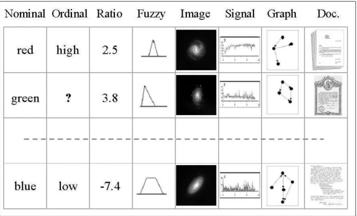
A visual virtual reality based data mining technique extending the concept of 3D mod-eling to relational structures was presented in (Vald´es, 2002b), (Vald´es, 2003), (see also http://www.hybridstrategies.com). It is oriented to the understanding of large heteroge-neous, incomplete and imprecise data, as well as other forms of structured and unstructured knowledge. In this approach, the data objects are considered as tuples from a heterogeneous space (Vald´es, 2002a) Fig.1. A heterogeneous domain is a Cartesian product of a collection of source sets: ˆHn = Ψ
1× · · · × Ψn , where n > 0 is the number of information sources to consider.
A virtual reality space is the tuple Υ =< O, G, B,ℜm, g
o, l, gr, b, r >, where O is a rela-tional structure (O =< O, Γv >, O is a finite set of objects, and Γv is a set of relations); G is a non-empty set of geometries representing the different objects and relations; B is a
non-empty set of behaviors of the objects in the virtual world; ℜm ⊂ Rm is a metric space of dimension m (euclidean or not) which will be the actual virtual reality geometric space. The other elements are mappings: go : O → G, l : O → ℜm, gr : Γv → G, b : O → B.
Of particular importance is the mapping l, where several desiderata can be considered for building a VR-space. From a supervised point of view, l could be chosen as to emphasize some measure of class separability over the objects in O (Jianchang & Jain, 1995), (Vald´es, 2003). From an unsupervised perspective, the role of l could be to maximize some metric/non-metric structure preservation criteria (Kruskal, 1964), (Chandon & Pinson, 1981), (Borg & Lingoes, 1987), or minimize some measure of information loss (Sammon, 1969), defined to be: Sammon error = P 1 i<jδij P i<j(δij − ζij)2 δij (1)
where δij is a disimilarity measure in the original space between any objects i, j and ζij a disimilarity measure in the new space (the virtual reality space) between the images of objects i, j. Typically, classical algorithms have been used for directly optimizing such mea-sures: Steepest descent, Conjugate gradient, Fletcher-Reeves, Powell, Levenberg-Marquardt, and others. However, they suffer from local extrema entrapment. A hybrid approach was introduced in (Vald´es, 2004) combining Particle Swarm Optimization with classical
opti-mization (local search) techniques. The l mappings obtained using approaches of this kind are only implicit, as no functional representations are found. However, explicit mappings can be obtained from these solutions using neural network or genetic programming techniques. An explicit l is useful for both practical and theoretical reasons.
3
Multi-objective Optimization
Using Genetic Algorithms
A genetic algorithm permits particular sequences of operations on individuals of the current population in order to construct the next population in a series of evolving populations. The classical algorithm requires each individual to have one measure of its fitness, which enables the algorithm to select the fittest individuals for inclusion in the next population. An enhancement is to allow an individual to have more than one measure of fitness. The problem then arises for determining which individuals should be included within the next population, because a set of individuals contained in one population exhibits a Pareto Front(Pareto, 1896) of best current individuals, rather than a single best individual. Most (Burke & Kendall, 2005) multi-objective algorithms use the concept of dominance when addressing this problem.
A solution ↼
functions < f1(↼x), f2(↼x), ..., fm(
↼
x) > if 1. ↼
x(1) is not worse than ↼x(2) over all objectives.
For example, f3(↼x(1)) ≤ f3(↼x(2)) if f3(↼x) is a minimization objective. 2. ↼
x(1)is strictly better than↼x(2)in at least one objective. For example, f6(↼x(1)) > f6(↼x(2)) if f6(↼x) is a maximization objective.
One particular algorithm for multi-objective optimization is the elitist non-dominated sorting genetic algorithm (NSGA-II) (Deb, Pratap, Agarwal, & Meyarivan, 2000), (Deb, Agarwal, Pratap, & Meyarivan, 2000), (Deb, Agarwal, & Meyarivan, 2002), (Burke & Kendall, 2005). It has the features that it i) uses elitism, ii) uses an explicit diversity preserving mechanism, and iii) emphasizes the non-dominated solutions.
4
Multi-objective Optimization of Neural Networks for
Space Transformation
In the supervised case, a natural choice for representing the l mapping is an NDA neural network (Webb & Lowe, 1990), (Mao & Jain, 1993), (Mao & Jain, 1995), (Jain & Mao, 1992). The classical backpropagation approach to building NDA networks suffers from the well known problem of local extrema entrapment. This problem was approached in (Vald´es
& Barton, 2005) with hybrid stochastic-deterministic feed forward networks (SD-FFNN). The SD-FFNN is a hybrid model where training is based on a combination of simulated an-nealing with the powerful minima seeking conjugate gradient, which improves the likelihood of finding good extrema while containing enough determinism. Clearly, the problem can be approached from an evolutionary computation perspective with networks trained with evo-lution strategies, particle swarm optimization, and others. In particular genetic algorithms may be used.
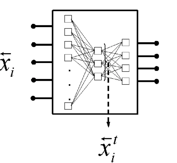
The output of both the output layer and the last hidden layer are exported (Fig. 2) and are used for computing two different error measures.
The collection of last hidden layer outputs is the image of the data matrix in the original n-dimensional space, to the usually lower m-dimensional Euclidean subspace defined by the hypercube with sides conditioned by the range of the activation function operating in the last hidden layer. A similarity (dissimilarity) measure can be defined for the patterns in the transformed space and an error measure w.r.t another measure in the original space can be computed for evaluating the structure preservation (loss) associated with the transformation performed by the collection of hidden layers of the network. In this paper, the Sammon Error (Eq.1) was the measure used for characterizing dissimilarity loss.
5
Genetic Programming
Analytic functions are among the most important building blocks for modeling, and are a classical form of knowledge. Direct discovery of general analytic functions can be approached from a computational intelligence perspective via evolutionary computation. Genetic pro-gramming techniques aim at evolving computer programs, which ultimately are functions. Among these techniques, gene expression programming (GEP) is appealing (Ferreira, 2002). It is an evolutionary algorithm as it uses populations of individuals, selects them according to fitness, and introduces genetic variation using one or more genetic operators. GEP individ-uals are nonlinear entities of different sizes and shapes (expression trees) encoded as strings of fixed length. For the interplay of the GEP chromosomes and the expression trees (ET), GEP uses a translation system to transfer the chromosomes into expression trees and vice versa (Ferreira, 2002). The set of operators applied to GEP chromosomes always produces valid ETs.
The chromosomes in GEP itself are composed of genes structurally organized into a head and a tail (Ferreira, 2001). The head contains symbols that represent both functions (from a function set F) and terminals (from a terminal set T), whereas the tail contains only terminals. Two different alphabets occur at different regions within a gene. For each problem, the length of the head h is chosen, whereas the length of the tail t is a function of h and the number of arguments of the function with the largest arity.
As an example, consider a gene composed of the function set F={Q, +, −, ∗, /}, where Q represents the square root function, and the terminal set T={a, b}. Such a gene (the tail is shown in bold) is: *Q-b++a/-bbaabaaabaab, and encodes the ET which corresponds to the mathematical equation f (a, b) =√b ·¡¡a + b
a ¢
− ((a − b) + b)¢ simplified as f (a, b) = b·√b a
GEP chromosomes are usually composed of more than one gene of equal length. For each problem the number of genes as well as the length of the head has to be chosen. Each gene encodes a sub-ET and the sub-ETs interact with one another forming more complex multi-subunit ETs through a connection function. To evaluate GEP chromosomes, different fitness functions can be used.
6
Application to Earth Sciences:
Geophysical Prospecting
The previously described approach was applied to geophysical data obtained from an in-vestigation dealing with the detection of underground caves. Karstification is a peculiar geomorphological and hydrogeological phenomenon produced by rock solution as the dom-inant process. As a consequence, the earth‘s surface is covered by irregular morphologies, like lapiaz, closed depressions(dolinas), sinks, potholes and underground caves. The hydro-graphic network is usually poorly developed, and rain waters infiltrate to form an
under-ground drainage system. Sometimes the caves are opened to the surface, but typically they are buried, requiring the use of geophysical methods. Cave detection is a very important problem in civil and geological engineering.
The studied area contained an accessible cave and geophysical methods complemented with a topographic survey were used with the purpose of finding their relation with subsurface phenomena (Vald´es & Gil, 1982). This is a problem with partially defined classes: the existence of a cave beneath a measurement station is either known for sure if made over the known cave, or unknown since there might be a buried cave beneath. Accordingly, only one class membership is defined.
The set of geophysical methods included 1) the spontaneous electric potential (SP) of the earth‘s surface measured in the dry season, 2) the vertical component of the electro-magnetic field in the Very Low Frequency (VLF) region of the spectrum, 3) the SP in the rainy season, 4) the gamma radioactive intensity and 2) the local topography. These four physical fields, along with the surface topography, were the five variables to be used in the study. In the area, a gentle variation in geological conditions for both the bedrock and the overburden was suspected by geologists. An isolation of the different geophysical field sources was necessary in order to focus the study on the contribution coming from underground targets, in an attempt to minimize the influence of both the larger geological structures and the local heterogeneities.
6.1
Data Preprocessing
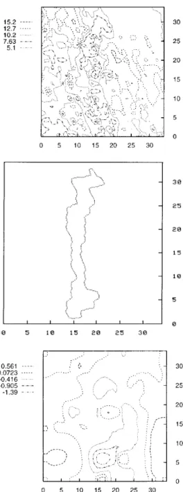
The complexity of these measured geophysical fields in the area is illustrated by the dis-tribution of the standard scores corresponding to the gamma ray intensity and the surface topography. While radioactivity is highly noisy, topography shows few features. Both fields are shown in Fig.3 (top and bottom). Since the geophysical fields are measured using dif-ferent units, in order to neutralize the effect of the difdif-ferent scales introduced by the units of measurement, all values were transformed to standard scores (i.e. to variables with zero mean and unit variance).
Each geophysical field was assumed to be described by the following additive two-dimensional model composed of trend, signal, and random noise: f (x, y) = t(x, y) + s(x, y) + n(x, y). where f is the physical field, t is the trend, s is the signal, and n is the random noise component, respectively. To isolate an approximation of the signals produced by the un-derground target bodies, a linear trend term ˆt(x, y) = c0 + c1x + c2y was fitted (by least squares) and subtracted from the original field. The residuals ˆr(x, y) = f (x, y) − ˆt(x, y) were then filtered by direct convolution with a low pass finite-extent impulse response two-dimensional filter to attenuate the random noise component. Such convolution is given by ˆ
s(x, y) = PNk1=−NPNk2=−Nh(k1, k2)ˆr(x − k1, y − k2) where ˆr(x, y) is the residual, ˆs(x, y) is the signal approximation, and h(k1, k2) is the low-pass zero-phase shift filter.
was used for analysis. In total, 1225 points in a regular grid were measured for the five physical fields previously mentioned. As a last preprocessing step, the data was clustered with a simple clustering method (the leader algorithm (Hartigan, 1975)). This algorithm operates with a dissimilarity or similarity measure and a preset threshold. A single pass is made through the data objects, assigning each object to the first cluster whose leader (i.e. representative) is close enough (or similar enough) to the current object w.r.t. the specified measure and threshold. If no such matching leader is found, then the algorithm will set the current object to be a new leader; forming a new cluster. In particular, for heterogeneous data involving mixtures of nominal and ratio variables, the Gower similarity measure (Gower, 1971) has proven to be suitable. For objects i and j the similarity is given by
Sij = p X k=1 sijk/ p X k=1 wijk (2)
where the weight of the attribute (wijk) is set equal to 0 or 1 depending on whether the comparison is considered valid for attribute k. If vk(i), vk(j) are the values of attribute k for objects i and j respectively, an invalid comparison occurs when at least one of them is missing. In this situation, wijk is set to 0. For quantitative attributes (like the ones of the datasets used in the paper), the scores sijk are assigned as sijk = 1 − |vk(i) − vk(j)|/Rk where Rk is the range of attribute k. For nominal attributes sijk = 1 if vk(i) = vk(j), and 0
otherwise.
The Gower’s similarity measure was used with a threshold value of 0.97. As a result, 648 leaders (cluster representatives) were found, corresponding to a subset of the original data. This smaller data set retains most of the original similarity structure because of the high threshold value.
7
Main Results
A series of multi- and single objective experiments were performed in order to study some of the properties of the data used within this study.
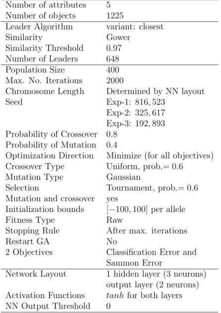
The experimental settings for the multi-objective experiments are shown in Table-1, which comprise a description of the data, the leader algorithm options, the evolutionary multi-objective optimization options, and the two objective function parameters, including the parameters used for non-linear discriminant analysis.
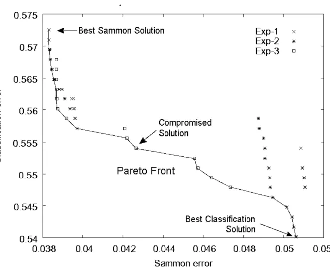
The 3 multi-objective experiments each generate approximately 10 distinct multi-criteria solutions, which lead to a total of approximately 30 distinct solutions for the multi-criteria problem. Fig-4 shows the solutions and the resulting Pareto Front for the two objective func-tions (neural network classification error and sammon error of the constructed space w.r.t. the original space dissimilarity matrix) that were obtained by the NSGA-II algorithm(Deb,
Pratap, et al., 2000). Three solutions were selected from Fig-4
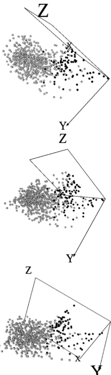
that represent the two extremes and a compromise of these two objectives. These selec-tions were then each visualized by constructing a 3-dimensional VR space from the hidden layer of the neural network solutions as shown in Fig-5. The leftmost representation in Fig-5 shows the best multi-objective Sammon error solution, with the property of preserving data structure. While the rightmost representation shows the best multi-objective classification error solution; a space in which objects should be maximally separated in terms of their class membership (cave or unknown). The middle representation demonstrates a multi-objective compromised solution that attempts to both preserve the original data structure and separate the objects as much as possible w.r.t. class membership.
The extremal solutions found by multi-objective optimization as reported in Fig-4 were then compared to single-objective counterparts. In particular, the best structure preserva-tion multi-objective solupreserva-tion was compared with a solupreserva-tion obtained by a single-objective optimization algorithm.
Table-2 presents the experimental settings used for the single-objective algorithm, in this case Fletcher-Reeves (Press, Flannery, Teukolsky, & Vetterling, 1986). The resulting 3-dimensional Fletcher-Reeves VR space is shown as the representation on the bottom of Fig-6. It has a lower Sammon error of 0.0266 compared to the multi-objective solution of 0.0383 and can be seen to contain a more pointed extremity on the right, indicating the
original data structure nature.
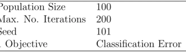
The best classification preservation multi-objective solution was also compared to a single-objective counterpart. The experimental settings for the single-single-objective optimization of classification error are shown in Table-3. The top of Fig-7 shows the best multi-objective classification error solution, while the bottom shows a representation of the best single-objective solution. That is, the output of the hidden layer of the non-linear discriminant analysis feed forward neural network was orthogonalized w.r.t. variance via principal com-ponent analysis and then plotted in the 3 dimensional VR space as shown on the bottom of Fig-7. Overall, the top and bottom VR spaces generally separate the spaces into two regions, with the cave objects on the right and the unknown objects on the left. There are some unknown objects that have very similar properties as the cave objects, indicating potential prognostic ability of the two spaces. In addition, the single-objective solution can be seen to strongly polarize the space into the cave and unknown classes. In particular, with the exception of one cave object (see arrow in Fig-7), all of the cave objects are clustered within a circled region of the space. The other pole of the space can be seen to contain another cluster of more densely packed objects. This other cluster represents objects that can be most dramatically non-linearly separated in terms of class structure from the cave objects, indicating their “non-caveness”.
in single-objective mode (targeting a 3D new space) can be described by:
X = ϕx(v1, v2, v3, v4, v5) Y = ϕy(v1, v2, v3, v4, v5) Z = ϕz(v1, v2, v3, v4, v5)
where {v1, v2, v3, v4, v5} are the original variables (i.e. the transformed physical fields), X, Y, Z are the variables in the new space, and ϕx, ϕy, ϕz are the non-linear functions of the original variables defining the mapping performed by the NDA neural network. The distribution of the data in the transformed space reveals a clearly polarized structure, which is further refined by the principal component (PC) transformation which was applied to the X, Y, Z variables of the new space, to create yet another new space (the principal components space).
P C1 = ψ1(ϕx, ϕy, ϕz) = ψ1 ◦ ←−ϕ P C2 = ψ2(ϕx, ϕy, ϕz) = ψ2 ◦ ←−ϕ P C3 = ψ3(ϕx, ϕy, ϕz) = ψ3 ◦ ←−ϕ
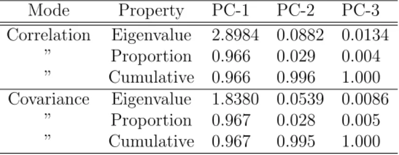
a whole, the process is expressed by a transformation given by function compositions ψi◦ ←ϕ ,− where i ∈ [1, 3]. It is clear from Table-4 that the first component accounts for about 97% of the total variance, thus explaining the separation of the elements of the cave and unknown classes.
The NDA transformed space (Fig-7 bottom) shows a remarkable polarization of the pattern vectors in two half spaces. The rightmost half space contains all of the vectors corre-sponding to the known class (cave) which on the other hand have the positive values of the first PC. Moreover, almost all of the vectors of the cave class reside at the very extreme of the distribution, thus exhibiting the largest positive values of the first PC. The leftmost half space is composed only of elements of the unknown class, with negative values of the first component. The very nature of the NDA network indicates that these vectors correspond to measurements made on sites much less likely to have a cave underneath, and there is a densely packed cluster of such objects exhibiting the largest negative values. There is a much less dense middle space in between the two extremes representing the elements whose prop-erties do not allow a clear distinction, therefore conforming an undecidable region. Clearly, the value of the first principal component is a measure of the degree of ”cavehood” expected for the corresponding vector of the transformed physical fields, and accordingly, its spatial distribution should give an indication about where to expect the presence of other caves, not yet opened to the surface. The distribution of the nonlinear composition ψ1 ◦ ←ϕ over the−
studied area is shown in Fig- 8(left). This first principal component representings roughly 96.7% of the variance of the best non-linear discriminant neural network solution (which provides 3 non-linear attributes from the original 5) as found by the single objective (clas-sification error minimization) optimization algorithm. There is a clear a central ridge of high values coinciding with the zone where the known cave is located, and a fading hallo as the distance from the cave increases, until it becomes almost nonexistent at the East-West borders. Geologically, this result is consistent with the nature of the karstification process, and the very fuzzy nature of geological boundaries, as known from ore and other kind of underground deposits. As such, the ψ1◦ ←−ϕ function can be used as a base for constructing a data-driven fuzzy membership function for the cavehood property. In addition, it is in-teresting to observe the presence of an almost circular feature at the central-left portion of Fig- 8, exhibiting high positive ψ1◦ ←ϕ values, suggesting the potential presence of buried− caves in that area. A borehole drilled at that location hit a buried cavity.
7.1
Gene Expression Programming Results
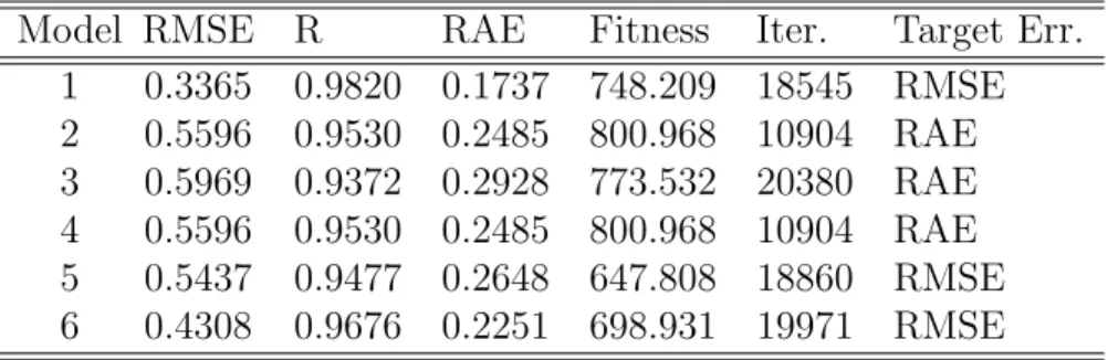
In order to obtain a more precise mathematical description of the ψ1◦ ←ϕ function, genetic− programming in the variant of GEP was applied with the purpose of finding a compact analytical representation of the composite mapping. Several experiments were performed targeting root mean squared error (RMSE) and relative absolute error (RAE) minimization.
The results are shown in Table 5
In particular, Model-1 has low RMSE, as well as the highest correlation, therefore rep-resenting a good approximation to the combined action of the NDA neural network, in functional composition with the PC orthogonal transformation. The analytic approximation to ψ1◦ ←ϕ function is given by the expression:−
d (ψ1◦ ←ϕ )(v− 1, v2, v3, v4, v5) = v2(k1+ v2) k2− v4 + v0 cos (v4+ v1+ sin (v2)) + k3 (3) + (sin (v1+ v4) + v4+ v1) sin (k4)
with the constants k1 = 2.304687, k2 = −6.591217, k3 = −2.893525 and k4 = 3.815918. The spatial distribution of this function is shown in Fig-8 (right), which remarkably approximates the original distribution obtained by the compositional application of the NDA network and the PC orthogonal transformation. The features corresponding to the known cave and the circular anomaly (where the previously unknown cave was found) are completely retained by the analytic function ψ1◦ ←ϕ , evidencing the effectiveness of the GEP approach.−
8
Conclusions
The combination of several computational intelligence approaches such as NDA neural net-works, multi-objective optimization using genetic algorithms proved to be very effective for constructing new feature spaces for visual data mining. In particular, spaces oriented to maximize structure preservation (using the last hidden layer output of the NDA network) and classification accuracy (using the network’s output layer) simultaneously can be con-structed using the set of solutions lying along the Pareto front, even for real world problems with partially defined classes. Complex properties like those obtained by successive applica-tion of different nonlinear and linear mappings can be approximated effectively by genetic programming techniques like GEP.
Acknowledgment
The authors would like to thank Robert Orchard from the Integrated Reasoning Group (Na-tional Research Council Canada, Institute for Information Technology) for his constructive criticism of the first draft of this paper.
References
Borg, I., & Lingoes, J. (1987). Multidimensional similarity structure. Springer-Verlag. Burke, E., & Kendall, G. (2005). Search methodologies: Introductory. New York: Springer
Science and Business Media, Inc.
Chandon, J., & Pinson, S. (1981). Analyse typologique. th´eorie et applications. Masson, Paris.
Deb, K., Agarwal, S., & Meyarivan, T. (2002). A fast and elitist multi-objective genetic algorithm: Nsga-ii. IEEE Transactions on Evolutionary Computation, 6 (2), 181–197. Deb, K., Agarwal, S., Pratap, A., & Meyarivan, T. (2000, September). A fast elitist non-dominated sorting genetic algorithm for multi-objective optimization: Nsga-ii. In Proceedings of the parallel problem solving from nature vi conference (pp. 849–858). Paris, France.
Deb, K., Pratap, A., Agarwal, S., & Meyarivan, T. (2000). A fast and elitist multi-objective genetic algorithm: Nsga-ii (Tech. Rep. No. 2000001). Kanpur, India: Kanpur Genetic Algorithms Laboratory(KanGAL), Indian Institute of Technology.
Ferreira, C. (2001). Gene expression programming: A new adaptive algorithm for problem solving. Journal of Complex Systems, 13 (2), 87–129.
Ferreira, C. (2002). Gene expression programming: Mathematical modeling by an artificial intelligence. Angra do Heroismo, Portugal.
Gower, J. (1971). A general coefficient of similarity and some of its properties. Biometrics, 1 (27), 857–871.
Hartigan, J. (1975). Clustering algorithms. John Wiley & Sons.
Jain, A. K., & Mao, J. (1992). Artificial neural networks for nonlinear projection of multi-variate data. Baltimore, MD.
Jianchang, M., & Jain, A. (1995). Artificial neural networks for feature extraction and multivariate data projection. IEEE Transactions On Neural Networks, 6 (2), 1–27. Kruskal, J. (1964). Multidimensional scaling by optimizing goodness of fit to a nonmetric
hypothesis. Psichometrika(29), 1–27.
Mao, J., & Jain, A. K. (1993, March). Discriminant analysis neural networks. San Francisco, California.
Mao, J., & Jain, A. K. (1995). Artificial neural networks for feature extraction and multi-variate data projection. IEEE Transactions on Neural Networks, 6, 296–317.
Pareto, V. (1896). Cours d’economie politique. Rouge, Lausanne.
Press, W. H., Flannery, B. P., Teukolsky, S. A., & Vetterling, W. T. (1986). Numerical recipes in c. New York: Cambridge University Press.
Sammon, J. W. (1969). A non-linear mapping for data structure analysis. IEEE Transactions on Computers, C18, 401–408.
observational models. Neural Network World, 12 (5), 499–508.
Vald´es, J. J. (2002b, November). Virtual reality representation of relational systems and decision rules. Prague.
Vald´es, J. J. (2003). Virtual reality representation of information systems and decision rules. In Lecture notes in artificial intelligence (Vol. 2639, pp. 615–618). Springer-Verlag. Vald´es, J. J. (2004, September). Building virtual reality spaces for visual data mining with
hybrid evolutionary-classical optimization: Application to microarray gene expression data. Marbella, Spain: ACTA Press, Anaheim, USA.
Vald´es, J. J., & Barton, A. J. (2005). Virtual reality visual data mining with nonlinear discriminant neural networks: Application to leukemia and alzheimer gene expression data. Montreal, Canada.
Vald´es, J. J., & Gil, J. L. (1982). Application of geophysical and geomathematical methods in the study of the insunza karstic area (la salud, la habana). In Proceedings of the first international colloquium of physical-chemistry and karst hydrogeology in the caribbean region (pp. 376–384). La Habana.
Webb, A. R., & Lowe, D. (1990). The optimized internal representation of a multilayer classifier. Neural Networks, 3, 367–375.
Table 1: Experimental settings for i) the input data ii) the leader algorithm, iii) the evolu-tionary multi-objective optimization algorithm (NSGA-II), and iv) the objective functions (e.g. the non-linear discriminant analysis).
Number of attributes 5
Number of objects 1225
Leader Algorithm variant: closest
Similarity Gower
Similarity Threshold 0.97
Number of Leaders 648
Population Size 400
Max. No. Iterations 2000
Chromosome Length Determined by NN layout
Seed Exp-1: 816, 523
Exp-2: 325, 617 Exp-3: 192, 893 Probability of Crossover 0.8
Probability of Mutation 0.4
Optimization Direction Minimize (for all objectives)
Crossover Type Uniform, prob.= 0.6
Mutation Type Gaussian
Selection Tournament, prob.= 0.6
Mutation and crossover yes
Initialization bounds [−100, 100] per allele
Fitness Type Raw
Stopping Rule After max. iterations
Restart GA No
2 Objectives Classification Error and
Sammon Error
Network Layout 1 hidden layer (3 neurons) output layer (2 neurons) Activation Functions tanh for both layers NN Output Threshold 0
Table 2: Experimental settings for single objective optimization of Sammon error using the Fletcher-Reeves algorithm.
Optimization Method Fletcher-Reeves
Seed −16155
Maximum Number of Iterations 200
Absolute Error Threshold 0
Relative Error Threshold 0.000001 Dimension of the desired space 3
Table 3: Experimental settings for single objective optimization of classification error using a genetic algorithm. See Table-1 for the experimental settings not listed.
Population Size 100
Max. No. Iterations 200
Seed 101
Table 4: Principal components results for the NDA 3-D space. For all modes, the first component accounts about 97% of the total variance.
Mode Property PC-1 PC-2 PC-3 Correlation Eigenvalue 2.8984 0.0882 0.0134 ” Proportion 0.966 0.029 0.004 ” Cumulative 0.966 0.996 1.000 Covariance Eigenvalue 1.8380 0.0539 0.0086 ” Proportion 0.967 0.028 0.005 ” Cumulative 0.967 0.995 1.000
Table 5: Results of Gene Expression Programming experiments.
Model RMSE R RAE Fitness Iter. Target Err.
1 0.3365 0.9820 0.1737 748.209 18545 RMSE 2 0.5596 0.9530 0.2485 800.968 10904 RAE 3 0.5969 0.9372 0.2928 773.532 20380 RAE 4 0.5596 0.9530 0.2485 800.968 10904 RAE 5 0.5437 0.9477 0.2648 647.808 18860 RMSE 6 0.4308 0.9676 0.2251 698.931 19971 RMSE
Figure 1: An example of a heterogeneous database. Nominal, ordinal, ratio, fuzzy, image, signal, graph, and document data are mixed. The symbol ? denotes a missing value.
Figure 2: Feed forward neural network for 2-objective optimization. ~xi is an input pattern to the network, ci is the network-predicted class membership of the input vector as coded by the output network layer and ~xt
i is the output of the last hidden layer, representing a transformation of the input vector into another space.
Figure 3: Top: Distribution of the gamma ray intensity (standard scores). Middle: The cave (in arbitrary units). Bottom: Local topography (standard scores).
Figure 4: Three multiobjective optimization algorithm (NSGA-II) experiments. Seeds: Exp-1: 816, 523, Exp-2: 325, 617, and Exp-3: 192, 893 respectively. The Pareto Front is shown, from which 3 solutions were selected: Best Sammon error solution, Best classification error solution and a solution compromising the two objectives.
Figure 5: Selected multi-objective optimization algorithm (NSGA-II) solutions. Top: best Sammon error solution (Sammon error: 0.0383, Classif error: 0.5725). Bottom: best Clas-sificaton error solution (Sammon error: 0.0506, Classif error: 0.5401). Middle: Solution compromising both error measures (Sammon error: 0.0422, Classif error: 0.5556). Dark objects represent measuring stations over the known surveyed cave location. Light objects represent measuring stations over locations in which it is not known whether a cave exists underground. Geometry = spheres, Behavior = static.
Figure 6: Top: best Sammon error solution obtained by the multi-objective optimization algorithm. (Sammon error: 0.0383) Bottom: Fletcher-Reeves single-objective optimization Sammon error solution.(Sammon error: 0.0266) Dark and light object representation ex-plained in Fig-5. Geometry = spheres, Behavior = static.
Figure 7: Top: best Classification error solution obtained by multi-objective optimization. Bottom: Best single objective classification error solution obtained by nonlinear discriminant analysis for 3 dimensions; and then orthogonalized via principal component analysis. The objects representing measurements over the cave are located at the extreme right; with the exception of one known measurement located closer to the middle of the VR space. Dark and light object representation explained in Fig-5. Geometry = spheres, Behavior = static.
Figure 8: Left: Distribution of the (ψ1 ◦←ϕ ) function over the studied area. Note the− relatively circular anomaly at the central-left location. The 0 value defines the two half spaces described in Fig- 7(bottom) and could be seen as a crisp threshold for the fuzzy property of cavehood. Right: Distribution of (ψ1d◦←ϕ ) as obtained with GEP.−