Report on initial vulnerability assessment for each case study

HAL Id: hal-02597964

https://hal.inrae.fr/hal-02597964

HAL is a multi-disciplinary open access

archive for the deposit and dissemination of sci-entific research documents, whether they are pub-lished or not. The documents may come from teaching and research institutions in France or abroad, or from public or private research centers.

L’archive ouverte pluridisciplinaire HAL, est destinée au dépôt et à la diffusion de documents scientifiques de niveau recherche, publiés ou non, émanant des établissements d’enseignement et de recherche français ou étrangers, des laboratoires publics ou privés.

study

S. Liersch, F. Hattermann, I. Zsuffa, J. Cools, A. van Dam, R. Kaggwa, S.

Namaalwa, T. Hein, P. Winkler, B. Kone, et al.

To cite this version:

S. Liersch, F. Hattermann, I. Zsuffa, J. Cools, A. van Dam, et al.. Report on initial vulnerability assessment for each case study. [Research Report] irstea. 2010, pp.89. �hal-02597964�

Report on Initial Vulnerability

Assessment for Each Case Study

WETwin-Deliverable 5.1

Gonzalo Villa Cox Sylvie Morardet

Document Information

Title Initial Vulnerability Assessment for each Case Study

Lead authors Stefan Liersch (PIK), Fred Hattermann (PIK)

Contributors István Zsuffa and others

Deliverable number D5.1

Deliverable description Initial Vulnerability Assessment for Each Case Study Report number

Version number D5.1_V15

Due deliverable date Month 12 Actual delivery date June 2010

Work Package WP5

Dissemination level RE

Reference to be used for citation

Prepared under contract from the European Commission

Grant Agreement no 212300 (7th Framework Programme)

Collaborative Project (Small or medium-scale focused research project) Specific International Cooperation Action (SICA)

Start of the project: 01/11/2008 Duration: 3 years

Acronym: WETwin

Full project title: Enhancing the role of wetlands in integrated water resources management for twinned river basins in EU, Africa and South-America in support of EU Water Initiatives

CONTENTS

2.3.1 SRES regions 16 2.3.2 Downscaled Data to Country Level 29 2.4 Climate Projections ...35

2.4.1 Regional Scale 35 2.4.2 Case Study Scale 39 2.5 Conclusions...46 2.5.1 Population 46 2.5.2 GDP 47 2.5.3 Energy Consumption 47 2.5.4 Land Use 47 2.5.5 Climate 47 3 DPSIR ... 49 3.1 Introduction ...49

3.2 The Driving Forces – Pressures – States – Impacts - Responses (DPSIR) Scheme – a “Control Paradigm“ ...49

3.3 DPSIR Analysis at the WETwin Study Sites ...51

3.4.1 Climate change/variability 51 3.4.2 Drivers and Pressures of the social domain 51

3.4.3 Energy production 51

3.4.4 Agriculture 52

4 Storylines ... 55

4.1 The Aim of Storylines ...55

4.2 Example ...55

4.3 Storylines of the Malian Case Study ...56

4.3.1 Storyline 1 58 4.3.2 Storyline 2 58 4.3.3 Storyline 3 58 4.3.4 Storyline 4 (under consideration) 59 4.4 Storylines of the Ugandan Case Studies ...59

4.4.1 Nabajjuzzi case study 59 4.4.2 Namatala case study 61 4.5 Storylines of the South African Case Study ...62

4.6 Storyline of the Ecuadorian Case Study ...65

5 Initial Vulnerability / Impact Assessment ... 67

5.1 Mali...68

5.1.1 Important Future Drivers and Pressures 69 5.1.2 Vulnerability Framework 70 5.1.3 Qualitative Assessment 71 5.2 Uganda (Nabajjuzzi wetland)...76

5.2.1 Important Future Drivers and Pressures 76 5.2.2 Vulnerability Framework 76 5.2.3 Qualitative Assessment 77 5.3 Uganda (Namatala wetland)...81

5.3.1 Important Future Drivers and Pressures 81 5.3.2 Vulnerability Framework 81 5.3.3 Qualitative Assessment 82 5.4 South Africa...84

5.4.1 Important Future Drivers and Pressures 84

5.4.2 Vulnerability Framework 84

5.4.3 Qualitative Assessment 84

5.5 Ecuador...85

5.5.1 Important Future Drivers and Pressures 85

5.5.2 Vulnerability Framework 85

5.5.3 Qualitative Assessment 85

1 Introduction

Vulnerability and its causes play an essential role in determining impacts. Understanding vulnerability is therefore as important as understanding the future pressures such as climate and global change itself. The IPCC (McCarthy et al., 2001) defines vulnerability as 'the degree to which a system is susceptible to, or unable to cope with, adverse effects of climate change, including climate variability and extremes. Vulnerability is a function of the character, magnitude, and rate of climate variation to which a system is exposed, its sensitivity, and its adaptive capacity'. In order to adapt this definition to the requirements of the WETwin project, we substitute the term 'climate' by 'external and internal drivers'. Since, the assessment of vulnerability of WETwin case study areas is not only subject to climate change but global change in general, including also socio-economical aspects.

A qualitative assessment of the most relevant future drivers and pressures will be developed for each case study area. This includes a qualitative assessment of the internal pressures like changes in demography, economic development, regional water demands, and land use. Furthermore, the qualitative assessment includes external pressures, such as climate change and changes derived from global scenarios following socio-economic pathways, as defined by the Intergovernmental Panel on Climate Change (IPCC). For this purpose three global scenarios were developed which are in line with the IPCC SRES scenarios (Nakicenovic & Swart, 2000) but complemented with recent trends and ideas derived from Millennium Assessment Scenarios (Cork et al., 2005).

A set of projections into the future (scenarios) is defined for the most important drivers in the form of storylines applicable for the sites regions. The scenarios are then interpreted for the different sites. Since every projection into the future is associated with uncertainty, different scenarios have to be formulated to reproduce the range of possible changes and therefore to quantify the uncertainty. The final step is to quantify the different types of adaptive capacity in consultation with the local experts. Vulnerability assessment for the WETwin case study areas is a process including the following steps:

1. Development of global change scenarios (Chapter 2)

2. Development of DPSIR chains for each case study (Chapter 3) 3. Definition of site-specific storylines (Chapter 4)

4. Initial vulnerability/impact assessment for the southern case studies (Chapter 5)

The development of global change scenarios is important to determine boundary conditions for regional scenarios. The primary objective of the development of DPSIR chains (Driving force, Pressure, State, Impact, Response) is to identify and explore the major environmental and livelihood problems (impacts) at the study sites. Site-specific storylines are important to focus on specific research questions. According to Füssel (2007), it is fundamental to include four dimensions into the storylines in order to describe a vulnerable situation. Finally, these storylines support the development of regional scenarios. Indicators are necessary to quantify and/or qualify changes of the system state and are a fundamental basis for the vulnerability assessment.

2 Global Scenarios

Scenarios are a central component in assessment processes for a range of global issues, including climate change, biodiversity, agriculture, and energy (O'Neill et al., 2008). Global change scenarios play an essential role in vulnerability assessment of the WETwin case studies. They determine boundary conditions for scenario downscaling to the regional scale, and, together with site specific storylines, they form the basis for the development of regional socio-economic scenarios.

Three global change scenarios are outlined here that are designed to assist the development of regional scenarios – in collaboration with case study leaders and local experts. They describe possible future developments of the world and are basically in line with the IPCC-SRES scenarios (Nakicenovic & Swart, 2000). The scenarios were complemented with ideas and assumptions developed in the frame of the Millennium Assessment (MA) scenarios (Carpenter et al., 2005) which in turn use the IPCC-SRES scenarios as a basis for their assumptions about the energy and climate developments (Nelson, 2005). Furthermore, the three global change scenarios were supplemented with “new” future demographic trends and economic growth at the country level with respect to new insights (IIASA, 2007; Van Vuuren et al., 2007). The purpose of the illustration of these global storylines is to support and stimulate visions of how case study regions might develop in a changing world. For instance, liberalized world markets could lead to an increase of the production of agricultural goods in a certain region. In contrast to this, in a world with a focus on regional solutions and self-reliance, agricultural production of the same region might decrease, or the selection of produced goods is controlled by regional demands rather than oriented at world market prices. As the IPCC-SRES scenarios, the introduced global change scenarios are divided into globalization (G) or regionalization (R) and with focus on economy (Ec) or environment (Env). Following scenarios are outlined:

• G-Ec: globalization with focus on economy • G-Env: globalization with focus on environment • R-Ec: regionalization with focus on economy

Why using a terminology different from IPCC-SRES?

The assumptions formulated for each scenario are generally in line with the IPCC-SRES scenario storylines. Some trends underlying the SRES scenarios are not up to date and where modified after suggestions by (Arnell et al., 2004; van Vuuren et al., 2007). For instance: “the SRES land cover trends are consistent with the narrative storylines, they are inconsistent with recent trends. Under none of the storylines is there a sustained continued deforestation, for example, and crop areas decrease under all of them” (Arnell et al., 2004). Also there exist discontinuities in the IPCC-SRES scenarios regarding GDP growth rates. This mainly holds for Central America and Africa (van Vuuren et al., 2007).

Furthermore, the developed scenarios are complemented with stories from MA scenarios. Thus, ideas from different sources are mixed (without compromising the consistency of the scenarios). Consequently, new names were invented in order to avoid confusion.

Scenario development is a way to explore possibilities for the future that cannot be predicted by extrapolation of past and current trends (Cork et al., 2005). The comparison of different scenarios supports the understanding of potential impacts of today’s decisions on tomorrow’s ecosystems and human well-being (Carpenter et al., 2005). Scenarios offer a means for examining the forces shaping the world and the uncertainties that lie ahead (Ayeni et al., 2002). Some key issues to consider in the formulation of scenarios include: the boundary; the current state; the definition and determination of driving forces; the narrative, or storyline; and images of the future (Ayeni et al., 2002, Chapter 4). Ayeni et al. (2002) name three arguments why long-range future cannot be extrapolated: ignorance, surprise and volition.

• Insufficient information on both the current state of the system and on the forces governing its dynamics leads to a classical statistical dispersion over possible future scenarios.

• Even if precise information were available, complex systems are known to exhibit turbulent behaviour, extreme sensitivity to initial conditions and branching behaviours at various thresholds. Therefore, the possibilities for novelty, surprise and emergent phenomena make prediction impossible.

• The future is unknowable because it is subject to human choices that have not yet been made. A note for the excited reader: An interesting article about global scenario development was published

by Raskin (2008). The author proposes three scenarios (Conventional Worlds, Barbarization, Great Transitions) each with two variations.

2.2.1 G-Ec Scenario

The underlying assumptions for this scenario are generally in line with the IPCC-SRES scenario A1B. According to the A1 storyline and scenario family it describes a future world of very rapid economic growth, global population that peaks in mid-century and declines thereafter, and the rapid introduction of new and more efficient technologies. Baer (2009) describes the A1 storyline as representing the desired future of 'neoliberals' who prioritize market-driven economic growth. Major underlying themes are convergence among regions, capacity building, and increased cultural and social interactions, with a substantial reduction in regional differences in per capita income (IPCC, 2000). Just as the A1B scenario, the G-Ec scenario is not relying too heavily on one particular energy source (fossil intensive or non-fossil energy sources). Similar improvement rates applied to all energy supply and end use technologies is assumed. In addition to these assumptions some ideas from the “Global Orchestration” scenario (Cork et al., 2005) are included in the G-Ec scenario in order to present a more illustrative and more complete picture of this scenario.

Global liberalized markets are well developed and the society is worldwide connected. Hence, the focus is more on individuals rather than on states. Market regulations are only implemented where appropriate. Global cooperation improves social and economic well-being of all people and protects and enhances global public goods and services (such as public education, health, and infrastructure). The existence of supra-national institutions is usually an optimal precondition to deal with global environmental problems. But problems that have little apparent or direct impact on human well-being are given a low priority in favor of policies that directly improve well-being. Furthermore the approach to deal with environmental problems is reactive, hence, problems threatening human well-being are dealt with only after they become apparent. Humans strongly belief in the ability to find technological approaches to repair or replace lost ecosystem functions, (just as it always has in the past) and ecosystems are considered to be robust to the impacts of humans. The society runs the risk of underestimating environmental threats and is not well prepared for ecological surprises.

Increasing connections among people and nations at social, economic, and environmental scales hold benefits (such as economic prosperity, increasing equality, wealth, and global coordination) and risks (focus on global problems insufficient to sustain local and regional ecosystem services, breakdowns of ecosystem services create inequality, reactive management more costly than preventive or proactive approaches) at the same time (Cork et al., 2005).

Although there is a strong trend to social and economical convergence among regions, disparities will not completely disappear in the next decades. Hence, differences between poor and wealthy regions will remain with the consequences that poorer regions will still be more vulnerable to ecological and economical crisis.

2.2.2 G-Env Scenario

The underlying assumptions of the G-Env scenario are generally in line with the IPCC-SRES scenario B1. The B1 storyline and scenario family describes a convergent world with the same global population (as A1B or G-Ec, respectively) that peaks in mid- century and declines thereafter. Economic structures are oriented toward a service and information economy, with reductions in material intensity, and the introduction of clean and resource-efficient technologies. The emphasis is on global solutions to economic, social, and environmental sustainability, including improved equity, but without additional climate initiatives (IPCC, 2000). According to Baer (2009) the B1 scenario represents the desired future of globally oriented 'greens' who prefer deliberate efforts to achieve sustainability and greater equality. Additional ideas and assumption for the G-Env scenario are based on the “TechnoGarden” scenario (Cork et al., 2005).

The G-Env scenario is characterized by a connected world that strongly relies on technology and on highly managed and often-engineered ecosystems. Eco-efficiency is well developing. Solutions to environmental problems are usually technology-based. The strong feel for international cooperation is beneficial for reforms and policy initiatives resulting in good conditions to tackle global environmental problems. Environmental taxation and development of property rights to ecosystem services are important instruments to reduce pollution on the one hand and to support sustainable management and preservation of ecosystem functions on the other hand. Property rights are assigned to a diversity of individuals, corporations, communal groups, and states that act to optimize the value of their property. It is assumed that ecological management and engineering can be successful, although it does produce some ecological surprises that affect many people (Cork et al., 2005).

Similar to the G-Ec scenario there is an over-reliance on highly engineered systems and an overestimation on human technological capabilities to solve any environmental problem just in time. In contrast to the G-Ec scenario, environmental problems are often identified before they become severe.

What conditions at the beginning of the 21st century lead to the development of such a storyline? Poverty, inequality, and unfair global markets, together with environmental degradation, were pressing problems on the agendas of global and national decision-makers. “A key activity in which these issues intersected was agriculture. Agriculture was, and remains, the most extensive human modification on Earth's surface. World markets for agriculture were unequal. Trade barriers and perverse subsidies encouraged pollution in the rich world, impoverished rural communities, and undercut development in poor countries. A broad coalition of new-liberals, development advocates, and environmentalists organized against agribusiness to stimulate a global transformation of agriculture” (Cork, et al., 2005). New EU policies encouraged farmers to manage their land to produce a bundle of ecosystem services rather than focusing on crop production alone. People were paid for improving water quality by preserving key watersheds. Farmers realized that they could increase their income by receiving money to provide additional services. This increased the

expansion of multifunctional landscapes. Agriculture changed rapidly towards a balancing between food production and ecosystem services. Export subsidies and trade barriers were removed from global agricultural trade. The liberalization of agricultural markets leads to a huge growth in food imports into richer countries. Increasing investments from agribusiness in agriculture in Eastern Europe, Latin America, and Africa result in agricultural intensification. New varieties of existing crops were bred and locally adapted genetically modified crops and farming systems created. Profitability and farm production increases in Asia, Africa, and Latin America (Cork et al., 2005).

The G-Env scenario operates somewhat similarly to the G-Ec scenario, with substantial improvements in crop yields combined with a lower preference for meaty diets reducing pressure on crop area expansion. Increased food demand is also met through exchange of goods and technologies. Both calorie consumption levels and the reduction in the number of malnourished children are similar, albeit somewhat lower than in the G-Ec scenario.

Potential benefits of the G-Env scenario are: Win-win solutions to conflicts between economy and environment, optimization of ecosystem services, and societies that work with rather than against nature.

Potential risks are: Technological failures have far-reaching effects with big impacts, wilderness eliminated as “gardening” of nature increases, and people have little experience of non-human nature which leads to simple views of nature (Cork, et al., 2005).

2.2.3 R-Ec Scenario

The basic assumptions for this scenario are generally in line with the IPCC-SRES scenario A2. The A2 storyline and scenario family describes a very heterogeneous world. The underlying theme is self-reliance and preservation of local identities with less emphasis on economic, social, and cultural interactions between regions. Fertility patterns across regions converge very slowly, which results in continuously increasing global population (IPCC, 2000). In this storyline there is less emphasize on economic interactions between regions – compared to the other scenarios. Hence, economic development is uneven and primarily regionally oriented. Global average per capita income and per capita economic growth is more fragmented and slower than in other storylines. The income gap between industrialized and developing parts of the world does not narrow. Social and political structures diversify where some regions move toward stronger welfare systems and reduced income inequality, while others move toward “leaner” government and more heterogeneous income distributions (Nakicenovic and Swart, 2000). Due to the relatively low mobility of people, ideas, and capital technology diffuses rather slowly and technological change is heterogeneous. Although attention is given to potential local and regional environmental change, it is not uniform across regions and global environmental concerns are relatively weak.

Some ideas from the “Order from Strength” and “Adapting Mosaic” scenarios (Cork et al., 2005) are used to supplement the R-Ec storyline. Due to the low emphasis on international cooperation and social and cultural interactions, the regionalized and fragmented world is concerned with security and protection, emphasizing primarily regional markets, and paying little attention to the common goods. National environmental policies focus on securing natural resources seen as critical for human well-being. The environment issues are seen as secondary to other challenges. Just as in the G-Ec scenario, people strongly belief in the ability of humans to solve environmental challenges with technological measures. The approach to ecosystem management is generally reactive. But there is great regional variation in management techniques. Some local areas explore adaptive management, using experimentation, while others manage with command and control or focus on economic measures.

2.2.4 Benefits and Risks of Globalization, Regionalization, and Technological Progress

The arguments listed in the following tables do not claim to be complete. They were derived from the section additional insights emerging from scenarios (Cork et al., 2005).

Table 2.1. Some Benefits and Risks of Globalization

Benefit Risk

Increasing global cooperation and a focus on global public good is likely to improve overall human well-being.

Ecological crises can accentuate inequalities as they tend to affect poor regions and countries more than wealthy regions.

A global development that emphasizes environmental technology and engineered ecosystems will contribute to sustainable development by allowing for greater efficiency and optimal control of ecosystems.

Global development of environmental technology and engineered ecosystems may lead to losses in local, rural, and indigenous knowledge and cultural values.

Globally controlled institutions can be too large and rigid to respond effectively to ecological surprises, yet local institutions may neglect important linkages for anticipating and managing such surprises.

Table 2.2. Some Benefits and Risks of Regionalization

Benefit Risk

Local problems become more tractable, and can

be addressed by citizens. Emphasis on adaptive management and learning at local scales may be achieved at the cost of overlooking global problems that may result in global environmental surprises with serious local repercussions.

Protection of key natural resources in richer

regions could see an improvement. Attention to global problems such as climate change and marine fisheries may decrease, leading to increasing magnitude of their impacts. Strategies that focus on local and regional safety and protection may disregard cross-border and global issues, restrict trade and movement of people, and increase inequalities.

Regionalization might offer security in the face of

aggression, environmental pests, and diseases. Regionalization increases risks of longer-term internal and international conflict, ecosystem degradation, and declining human wellbeing. Local management of ecosystems provides

access to ecosystem services on local scales, but local strategies are more likely to be effective when accompanied by measures to ensure regional and global coordination.

and social disasters for several decades.

Table 2.3. Some Benefits and Risks of Technological Progress

Benefit Risk

Technological progress can improve and support

sustainable management of the environment. Increasing confidence in human ability to manage, tame, and improve nature may lead people to overlook factors that sometimes cause breakdowns of ecosystem services.

Green technology reduces emissions of

greenhouse gases. Large scale technological solutions carry the internal risks of failure and can engender technology-related ecological surprises. Genetically modified crops and farming systems

can increase agricultural productivity and contribute to food security.

Public acceptance of genetically modified crops is relatively low.

2.2.5 Comparison of the Three Global Scenarios

Table 2.4. Scenario Comparison (derived from IPCC (2000); Arnell et al. (2004); Cork et al. (2005))

G-Ec (A1B) (global/economic) R-Ec (A2) (regional/economic) G-Env (B1) (global/environment.) Population growth (see Figure 2.5)

Low High Low

Economic growth (see Figure 2.6)

Very high Medium (diverse) Low in developing countries; medium in industrialized countries

High

GDP growth per capita

and year (Figure 2.7) Ind.: US$ 817 _{Dev.: US$ 533} Ind.: US$ 332 _{Dev.: US$ 118} Ind.: US$ 514 _{Dev.: US$ 371} Service and information

economy High/medium Very high

Introduction of new

technologies Rapid Slow (diverse) Medium

Resource efficiency (see Figure 2.8 and Figure 2.9)

Resource availability High/medium Low Low

Energy use Very high/high High Low

Land use changes (see Figure 2.2 and Figure 2.4) Low-medium Cropland +3% Forest -2% Medium-high High Cropland -28% Forest +30% Global sustainability solutions to:

• Economy High/medium Low High

• Society High/medium Low High

• Environment High/medium Low High

Table 2.5. Economic Characteristics of the Three Scenarios (derived from Nakicenovic & Swart (2000); Cork et al., (2005))

G-Ec (A1B) R-Ec (A2) G-Env (B1)

A1 world invests its gains from increased productivity and know-how primarily in further

economic growth (high rates of investment and innovation in technology

→ rapid and successful economic development → rapid introduction of new and

more efficient technologies

The A2 world "consolidates" into a series of economic regions (differentiated world)

→ economic growth is uneven → slower technological change

(compared to A1) → technological change is

heterogeneous (more rapid than average in some regions and slower in others)

Fast-changing and convergent world

→ economic development is balanced

→ relatively smooth transition to alternative energy systems

Communication technology, advances in transport, and intensive mobility plays a central role

→ economic convergence results from these advances → relatively high level of

convergence in the per capita income levels

People, ideas, and capital are less mobile so that technology diffuses more slowly

→ low trade flows, relatively slow capital stock turnover (compared to A1)

Incentive systems, combined with advances in international institutions

→ rapid diffusion of cleaner technology

→ relatively high level of convergence in the per capita income levels Strong commitment to

market-based solutions Self-reliance in terms of resources → Regions with abundant

energy and mineral resources evolve more resource-intensive

economies, while those poor

High levels of economic activity → a higher proportion of this

income is spent on services rather than on material goods, and on quality rather than quantity, because the emphasis on material goods

in resources place a very high priority on minimizing import dependence Less emphasis on economic interactions between regions

is less

→ resource prices are

increased by environmental taxation

→ Massive income redistribution and

presumably high taxation levels may adversely affect the economic efficiency and functioning of world markets

Table 2.6. Socio-Economic Characteristics of the Three Scenarios (derived from Nakicenovic & Swart (2000); Cork et al.,

(2005))

G-Ec (A1B) R-Ec (A2) G-Env (B1)

Demographic and economic trends are closely linked, as affluence is correlated with long life and small families (low mortality and low fertility)

Fertility rates decline relatively

slowly Demographic transition to low mortality and fertility (same rate as in A1, but for different

reasons) it is motivated partly by social and environmental

concerns Regional average income per

capita converge and distinctions between "poor" and "rich" countries eventually dissolve

Income gap between now-industrialized and developing parts of the world does not narrow, (unlike in the A1 and B1)

High levels of economic activity and significant and deliberate progress toward international and national income equality (global income one-third lower than in A1).

Efforts to achieve equitable income distribution are effective. Strong welfare net prevents social exclusion on the basis of poverty.

High rates of investment and innovation in education / High savings and commitment to education at the household level

Social and political structures diversify; some regions move toward stronger welfare systems and reduced income inequality, while others move toward "leaner" government and more heterogeneous income

distributions

Investments in equity and social institutions

This world is not necessarily devoid of problems … problems of social exclusion, increased pressure on the global

commons...

People, ideas, and capital are less mobile and there is less emphasize on social and cultural interactions between regions

Governments, businesses, the media, and the public pay increased attention to the environmental and social aspects of development

Table 2.7. Environmental Characteristics of the Three Scenarios (derived from Nakicenovic & Swart (2000); Cork et al.,

(2005))

G-Ec (A1B) R-Ec (A2) G-Env (B1)

Energy and mineral resources are abundant in this scenario family because of rapid technical progress, which both reduces the resources needed to produce a given level of output and increases the economically recoverable reserves.

Regions with abundant energy and mineral resources evolve more resource-intensive economies, while those poor in resources place a very high priority on minimizing import dependence

The B1 world invests a large part of its gains in improved efficiency of resource use ("dematerialization"), and environmental protection (A1 world invests its gains from increased productivity and know-how primarily in further

economic growth) Rapid technological progress

"frees" natural resources

currently devoted to provision of human needs for other purposes

Self-reliance in terms of resources.

High-income but resource-poor regions shift toward advanced post-fossil technologies (renewables or nuclear), while low-income resource-rich regions generally rely on older fossil technologies.

Technological change and increased resource efficiency plays an important role. Reduced material wastage by maximizing reuse and recycling, reductions in pollution

Energy intensity decreases at an

average annual rate of 1.3% Final energy intensities decline with a pace of 0.5 to 0.7% per year.

Extensive use of conventional and unconventional gas as the cleanest fossil resource during the transition, but the major push is toward post-fossil technologies.

relatively smooth transition to alternative energy systems. Relatively low GHG emissions. The concept of environmental

quality changes in this storyline from the current emphasis on "conservation" of nature to active "management" of natural and environmental services, which increases ecologic resilience

Global environmental concerns are relatively weak, although attempts are made to bring regional and local pollution under control and to maintain environmental amenities

Incentive systems, combined with advances in international institutions, permit the rapid diffusion of cleaner technology

G-Ec (A1B) R-Ec (A2) G-Env (B1) Environmental amenities are

valued Although attention is given to potential local and regional environmental damage, it is not uniform across regions

High level of environmental and social consciousness and institutional effectiveness combined with a globally coherent approach to a more sustainable development including environmental and social aspects

With substantial food requirements, agricultural productivity is one of the main focus areas for innovation and research, development, and deployment (RD&D) efforts, and environmental concerns

Land use is managed carefully. Strong incentives for low-input, low-impact agriculture, along with maintenance of large areas of wilderness, contribute to high food prices with much lower levels of meat consumption than those in A1

2.3 Socio-Economic Projections

This chapter summarizes and illustrates existing projections of population development, GDP development, energy consumption, and land use change underlying the global change scenarios. Projected data are available at two different spatial scales, at the IPCC-SRES world region scale and/or at the country scale. Data on land use change and energy consumption are only available for IPCC-SRES world regions. Population and GDP development data are available for both the SRES regions and at the country level. Climate data projection is discussed in section 2.4.

2.3.1 SRES regions

The IPCC emissions scenarios include projections of various parameters at the scale of SRES regions (see Table 2.8 and Figure 2.1) and are based on the results of six integrated assessment models: AIM, ASF, IMAGE, MESSAGE, MINICAM, MARIA. A brief description of these models is given in Nakicenovic & Swart (2000).

Table 2.8. SRES Regions (Nakicenovic & Swart, 2000)

SRES Region Description

World World

OECD90 The OECD90 region groups together all countries that belong to the OECD as of 1990, the base year of the participating models, and corresponds to Annex II countries under UNFCCC (1992).

REF The REF region comprises those countries undergoing economic reform and groups together the East European countries and the Newly Independent States of the former Soviet Union. It includes Annex I countries outside Annex II as

defined in UNFCCC (1992).

ASIA The ASIA region stands for all developing (non-Annex I) countries in Asia.

ALM The ALM region stands for rest of the world and includes all developing (non-Annex I) countries in Africa, Latin America and the Middle East.

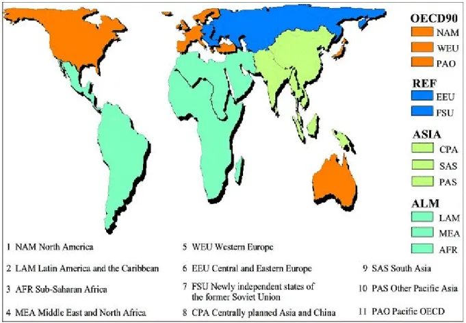
Figure 2.1. SRES regions, http://www.ipcc.ch/ipccreports/sres/emission/index.php?idp=90

According to the differentiation of SRES regions (Table 2.8 and Figure 2.1), the four southern WETwin case studies belong to the ALM region.

2.3.1.1 Land Use

According to Arnell et al. (2004) there are three issues in the application of the SRES world-region projections to estimate future land cover:

• Observed area of cropland summed across each region is greater than the baseline value used in the SRES projections.

• Everywhere within a major world region land use changes at the same rate. In practice, land cover change is likely to be greatest where population and population growth rates are greatest.

• There is a mismatch between recent trends and projected future cropland change in two of the SRES storylines (Levy et al., 2003).

According to Arnell et al. (2004) the SRES projections are very inconsistent with current trends and likely future patterns of land use change. The B1 scenario projects a decrease in cropland area and an increase in forest cover – which is consistent with the assumptions behind the scenarios but inconsistent with trends over the last century (Arnell et al., 2004). In some developing countries, especially in Africa, increase in input levels and intensification of production (of crop yields) are likely to continue for some time, but may also ultimately level off meaning that further increases in agricultural productivity will have to come through the expansion of land under cultivation. Demand for food, however, is allowed to vary between scenarios as it is linked to per capita GDP (Arnell et al., 2004) and population development. Deforestation of areas for permanent pasture rather than cropland may be a significant term, particularly in South America (Levy et al., 2004).

As reported by Levy et al., (2004) “there is large uncertainty in the future trend in cropland area as population increases. Until very recently, cropland area has shown a linear increase with population. However, in the last 50 years, in which the population has doubled, the increase in cropland area has been very small. How this trend will continue with a possible further doubling of the population over the next century is clearly highly uncertain”.

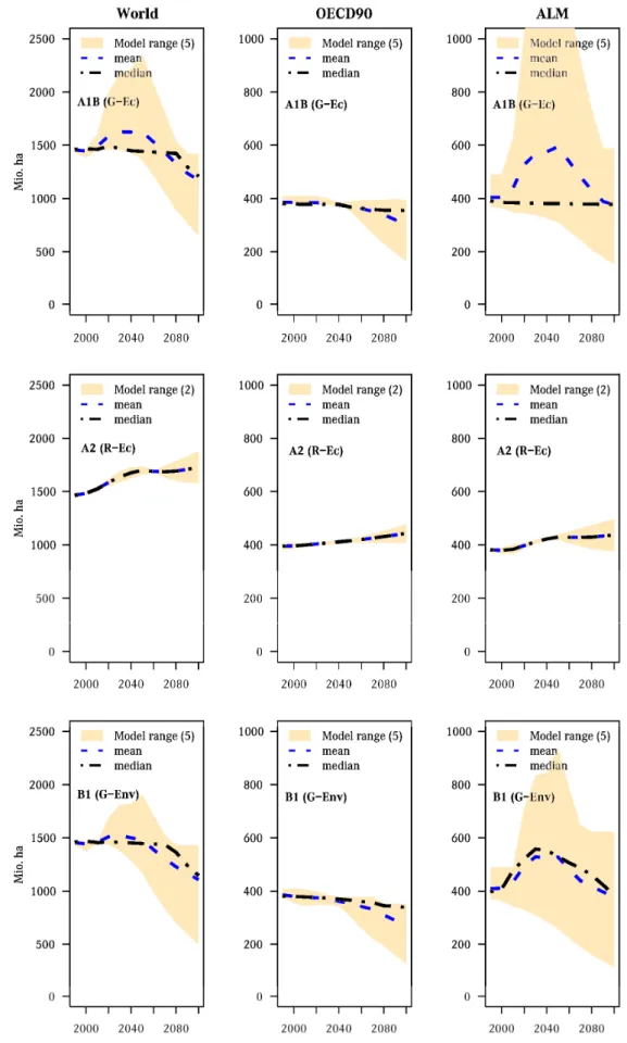
The following charts are illustrating the underlying assumption for the SRES regions World, OECD90, and ALM and the three scenarios: A1B (G-Ec), A2 (R-Ec), and B1 (G-Env). The data sources are results from the six integrated assessment models, where five models produce land cover trends for the A1B and B1 SRES scenarios and only two models for the A2 scenario. The projections show oftentimes large differences. Hence, in order to assess a general trend of change one should basically consider the median value. Corresponding data are available at: http://sres.ciesin.org/final_data.html.

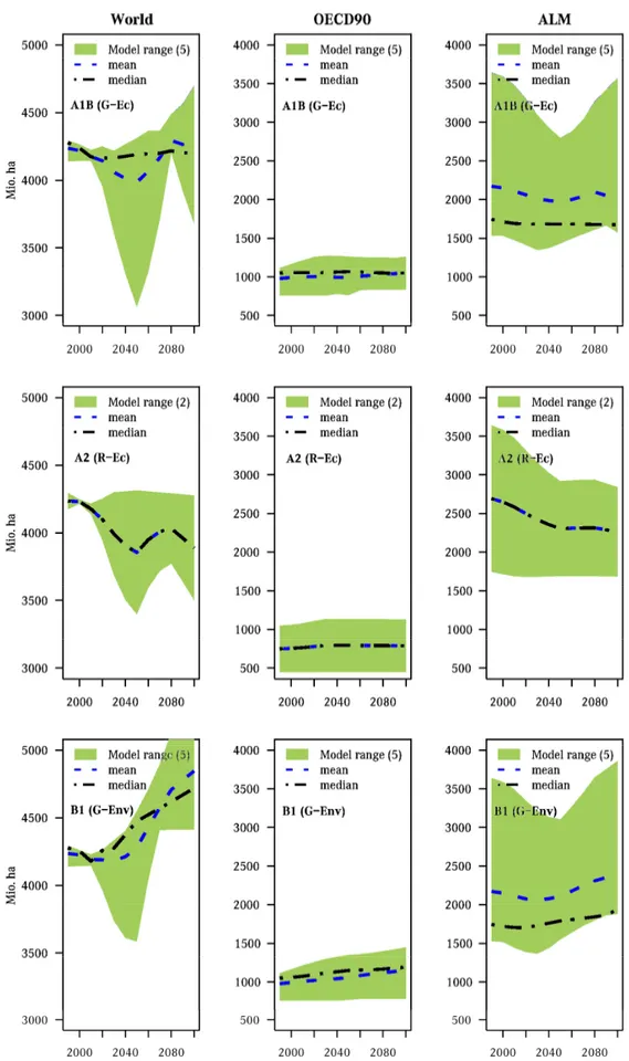
Figure 2.2 shows projections of cropland development underlying the three global change scenarios. The A1B (G-Ec) scenario shows no significant trends in all regions. In the A2 (R-Ec) scenario the cropland area is assumed to slightly increase in all regions. The B1 (G-Env) scenario shows a different pattern of change. There is a declining trend of cropland area projected for the OECD90 region and a rapid increase in the ALM region up to the year 2040. After 2040 cropland area in the ALM region is assumed to decrease until it reaches approximately the same extent as in 1990. As shown in Figure 2.3 the integrated assessment models start in the year 1990 already with a broad range of assumptions concerning the area of forest cover for the OECD90 and ALM region. Whereas there is almost accordance of forest area of the world in 1990. Due to the broad range of projections the results are highly uncertain. The A1B (G-Ec) scenario shows a slight decreasing trend for the ALM region and a slight increase of forest area for the OECD90 region. In the A2 (R-Ec) scenario the trend in forest area decrease is more significant for the ALM region and shows an increasing trend for OECD90 countries. An increasing trend of forest cover for all regions is assumed by the B1 (G-Env) scenario.

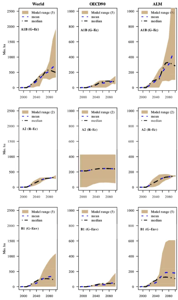
An increase of agricultural area used to produce energy biomass is assumed by all assessment models for all regions and all scenarios. Figure 2.4 illustrates these projections. The increasing trend is most significantly in the A1B (G-Ec) scenario. Regarding the model median the projections assume a maximum area of ~550 million hectare for the entire world at the end of the 21st century in the A1B (G-Ec) scenario. In the A2 (R-Ec) scenario the maximum extent is ~400 ha and in the B1 (G-Env) scenario ~300 ha. Furthermore, the models assume a more significant trend of increasing agricultural area used for energy biomass in the ALM region than in the OECD90 region.

2.3.1.2 Socio-Economic Development

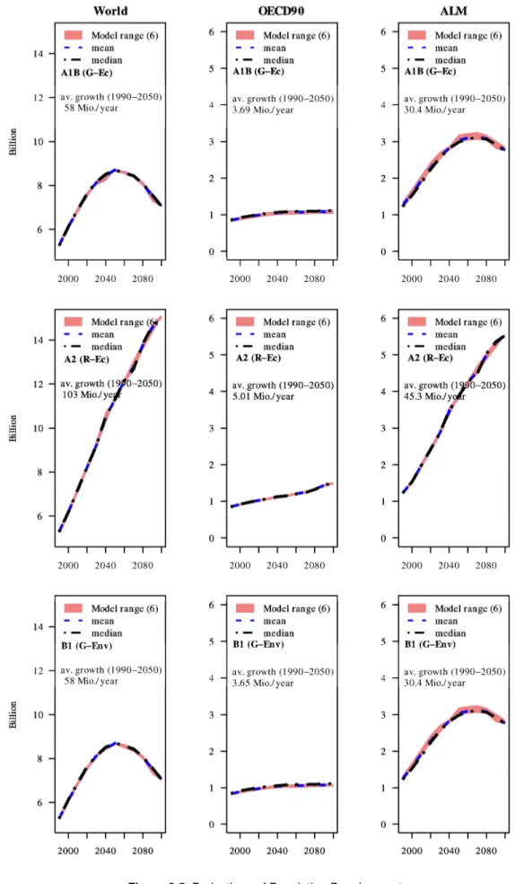
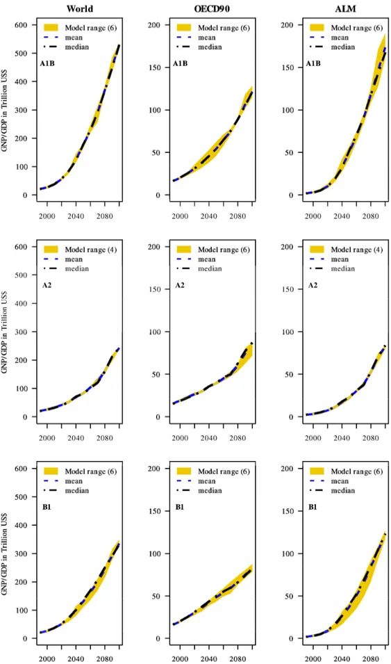
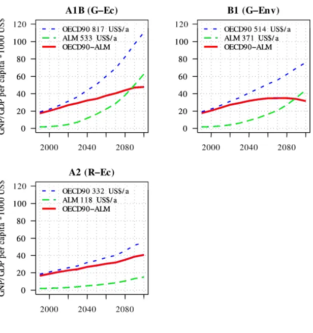
In contrast to the land use change projections, there is much higher agreement between the six assessment models for population development. The A1B (G-Ec) and B1 (G-Env) scenarios assume similar world population development with a peak in mid-century (~9 billion people) and a decline thereafter (see Figure 2.5). This trend is also projected for the ALM region, whereas population development in OECD90 countries is assumed to increase also after 2050 but at smaller growth rates. In all scenarios the average growth rates in the ALM region are much higher than in OECD90 countries. In the two globalization scenarios the growth rates between 1990 and 2050 are, with 30.4 Million people per year, eight times higher than in OECD90 countries (3.69 Million people per year). In the regionalization scenario the average growth rates are projected to be nine times higher in the ALM region than in the OECD90 region. The A2 (R-Ec) scenario projects an almost linear trend in world population growth, from ~6 billion in the year 2000 to ~15 billion at the end of the 21st century. Figure 2.6 illustrates projections of total GNP/GDP development for the three SRES regions. The A1B (G-Ec) scenario shows by far the highest growth rates of all scenarios. At the end of the 21st century total GNP/GDP is projected to be higher in the ALM region than in the OECD90 region in the two globalization scenarios (A1B/G-Ec and B1/G-Env). In the A2 (R-Ec) scenario GNP/GDP is projected to be equal between OECD90 and ALM countries. But note, that these are projections of total GNP/GDP. If we take population development into account and look at the GNP/GDP per capita instead of total GNP/GDP per region, the picture looks very different. As shown in Figure 2.7, the highest GNP/GDP per capita growth rates denotes the A1B (G-Ec) scenario, with an average growth rate of 817 US$ per capita and year in OECD90 countries and 533 US$ in the ALM region. In the B1 (G-Env) scenario average yearly GDP growth rates per capita are 514 US$ in OECD90 countries and 371 US$ in ALM countries. The average GDP growth rates are the lowest in the A2 (R-Ec) scenario, with 332 US$ per capita and year in OECD90 countries and 118 US$ in the ALM region. This scenario projects lower GDP growth rates for OECD90 countries than for the ALM regions in the two globalization scenarios.

The ratio of GDP per capita growth rates between the developing world (ALM region) and OECD90 countries (GDP growth ALM * 100 / GDP growth OECD90) can be considered as an indicator for the level of convergence between these two world regions. The highest ratio (72%) is projected for the B1 (G-Env) scenario, followed by the A1B (G-Ec) scenario with 65%, whereas the ratio in the A2 (R-Ec) scenario is only 36%. This might lead to the conclusion that the level of convergence is highest in the A1B (G-Ec) scenario and the lowest in the A2 (R-Ec) scenario. In reality, there is further divergence between OECD90 and ALM countries in all scenarios, because, although all regions denote increasing GDP growth rates, the pace of GDP per capita increase is higher in the developed world than in the developing world. Hence, we should conclude that the level of divergence between OECD90 and ALM countries is decreasing in the scenarios in the following order: 1. B1 (G-Env); 2. A1B (G-Ec); 3. A2 (R-Ec). The red line in Figure 2.7 shows the average differences of GDP development per capita and year between OECD90 and ALM countries (GDP per capita and year OECD90 minus GDP per capita and year ALM). In the A1B (G-Ec) scenario there was a difference of ~17,000 US$ GDP per capita per year in the base year 1990 between ALM and OECD90 countries. The difference projected for the year 2100, following an almost linear trend, is ~47,000 US$ per capita and year. In the A2 (R-Ec) scenario the trend is similar but the final difference in 2100 is “only” ~40,000 US$. The GDP gap increases in both scenarios! The B1 (G-Env) scenario is the only scenario where a real convergence trend is projected starting in mid-century. Up to 2060 there is an ongoing increase of divergence in GDP per capita and year between ALM and OECD90 countries, from ~17,000 US$ (1990) to ~35,000 US$ (2060). The period between the years 2060 and 2100 projects a trend of real convergence between ALM and OECD90 countries, where the difference of GDP per capita and year decreases from ~35,000 to ~30,000 US$.

Figure 2.7. GDP per Capita, Convergence or Divergence between OECD90 and ALM? Data source:

http://sres.ciesin.org/final_data.html

2.3.1.3 Energy Consumption

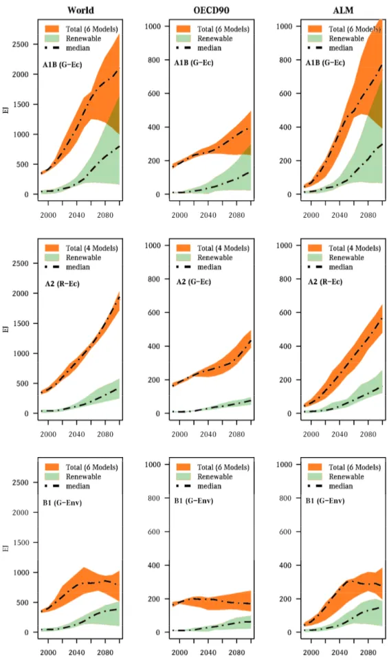
Figure 2.8 shows the future trends of total energy consumption and the share of renewable energy. The units are in Exajoule (1 EJ = 10^18 J). Total world energy consumption is projected to continuously increase in the A1B (G-Ec) and A2 (R-Ec) scenarios up to the end of the 21st century. The B1 (G-Env) scenario assumes increasing energy consumption up to mid-century and shows decreasing trends thereafter. The share of global renewable energy to total energy at the end of the 21st century is approximately 45% in the scenarios A1B (G-Ec) and B1 (G-Env), whereas the share in the A2 (R-Ec) scenario is projected to be ~20% only. It is worth noting that the A1B (G-Ec) scenario is the scenario with the highest energy consumption in 2100, although projected world population is only the half of the A2 (R-Ec) scenario at the end of the century. However, the uncertainties related to the projections of energy consumption, produced by the six assessment models, is rather large in the A1B (G-Ec) scenario. In both scenarios the energy consumption in OECD90 countries increases with almost similar patterns and the ALM region denotes very high total

energy consumption rates. The highest consumption rates for the ALM region are obtained in the A1B scenario. This might be a consequence of the rapid introduction of technology and increasing living standards in the developing world in this scenario.

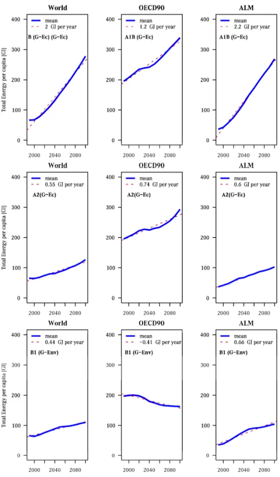
In the previous sub-section the level of convergence among SRES regions was assumed to be a function of GDP per capita development. If we use the per capita energy consumption as a measure to define convergence or divergence, respectively, the conclusions are slightly different. Figure 2.9 shows projected per capita energy consumption and their average growth rates in the three world regions. The two scenarios with a focus on economy (A1B/G-Ec and A2/R-Ec) project an increase of per capita energy consumption for all regions. The A1B (G-Ec) scenario shows by far the highest growth rates per capita and year (World = 2.2 GJ, OECD90 = 1.2 GJ, and ALM = 2.2 GJ). Global per capita energy consumption is projected to be almost three times higher than in the other two scenarios. However, a trend toward convergence between OECD90 and ALM countries can be denoted in the A1B (G-Ec) scenario, starting with a difference of ~150 GJ per capita in the base year 1990 and ending up with a difference of ~70 GJ in 2100. The strongest convergence according to the per capita energy consumption achieves the B1 (G-Env) scenario with 161 GJ in 1990 to 59 GJ in 2100. In contrast to this convergence trend in the globalization scenarios, the projections of energy consumption differences in the A2 (R-Ec) scenario increase from 158 GJ (1990) to 190 GJ in 2100.

2.3.2 Downscaled Data to Country Level

Aggregated population and GDP data used in the SRES report have been downscaled to the country level by CIESIN (2002), Van Vuuren et al. (2007), and Grübler et al. (2007). A description of the downscaling methods used by CIESIN (2002) and corresponding data are available at: http://www.ciesin.columbia.edu/datasets/downscaled/. Van Vuuren et al. (2007) used an external-input-based downscaling algorithm to downscale population data and a convergence-based downscaling method for GDP (per capita income levels) at the national level. Corresponding data are available from the authors. The downscaling method used by Grübler et al. (2007) is described in their article and corresponding data are available at IIASA (2007).

2.3.2.1 Population

The population directly influences the consumption of goods and emission levels and is thus an important driver of global environmental change. However, the IPCC-SRES scenarios are not longer fully reflecting current insights into possible future demographic trends (van Vuuren & O'Neill, 2006). Future population growth depends on a countries' phase of demographic transition. Many low-income countries are still in the transitional phase with a relatively young age structure. “The age profile of a population is one of the crucial factors in future population growth and represents a major reason for not applying linear downscaling to population projections” (Van Vuuren et al., 2007). The following charts illustrate population development at the country level for the four southern WETwin case study countries. Projections for the A2 scenario from IIASA (2007) correspond to the A2r scenario. IIASA (2007) data between decades have been linearly interpolated since they are available from 2000 to 2100 for each decade, whereas data from Van Vuuren (2007) and CIESIN (2002) are provided in five year steps between 1990 and 2100.

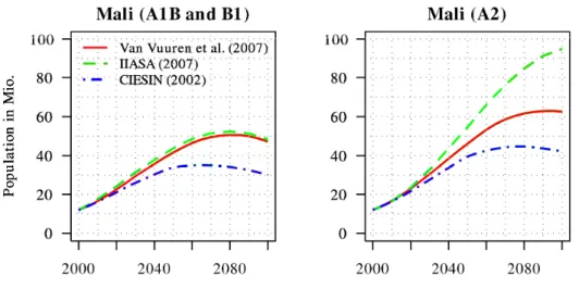
Figure 2.10. Population projections for Mali from three different sources

Mali’s population in 2009 was 13.4 million and the population growth rate is ~2.6% (CIA, 2010). Assuming a constant growth rate of 2.6% results in a population increase to 38.4 million people in 2050. Figure 2.10 shows exactly this trend for the A1B and B1 scenarios whereas Van Vuuren et al. (2007) and IIASA (2007) assume much more rapid increases for the A2 scenario. According to CityMayors (2010), Bamako, the capital of Mali with 1.8 million inhabitants, is currently estimated to

be the fastes growing city in Africa and the sixth fastest in the world (wikipedia.org). The projected average annual population growth for the period 2006 to 2020 is 4.45%.

Figure 2.11. Population projections for Uganda from three different sources

Uganda’s population in 2009 was 32.4 million and the population growth rate is ~2.7% (CIA, 2010). Assuming a constant growth rate of 2.7% results in a population increase to 96.6 million people in 2050. This assumption is in line with the projections shown in Figure 2.11 for the A1B and B1 scenarios. The projections of Van Vuuren et al. (2007) and CIESIN (2002) show almost the same trend for the A2 scenario (up to 2050) whereas the projections of IIASA (2007) assume a population increase up to 125 million people in 2050.

Figure 2.12. Population projections for South Africa from three different sources

The population of South Africa was 49 million in 2009 (CIA, 2010) and the growth rate is 0.28%. Following a constant growth rate the population in 2050 would increase to 55 million people. However, the projections for the A1B and B1 scenario are not in line with the assumption of a constant growth rate. IIASA (2007) and CIESIN (2002) assume a decreasing trend up to 2050 resulting in population decrease to approximately 40 million people (Figure 2.12). Van Vuuren et al. (2007) project an increase up to the year 2025 (55 million) and a decline thereafter with a population

of 51 million in 2050. For the A2 scenario IIASA (2007) and CIESIN (2002) project a population increase to approximately 50 million in 2050 whereas Van Vuuren et al. (2007) assume an increase to 68 million in 2050.

Figure 2.13. Population projections for Ecuador from three different sources

According to CIA (2010), the population of Ecuador was 14.6 million in 2009 and the growth rate was 1.5%. Assuming a constant growth rate of 1.5% would result in a population increase to 26.9 milion people in 2050. The same trend is assumed by Van Vuuren et al. (2007) and CIESIN (2002) for the A2 scenario, whereas IIASA (2007) projects an increase to approximately 23 million people in 2050 (Figure 2.13). The projections for the A1B and B1 scenarios assume a slower population increase up to 20 million people in 2050. Moreover, the projections show a decline of population after 2050.

2.3.2.2 GDP

The results of the methodology applied by van Vuuren et al. (2007) do not achieve improbable high income levels, as in the method used by Gaffin et al. (2004). Countries starting with a relatively large per capita income have lower income growth rates than countries starting with a relatively low per capita income. This is consistent with both the literature on conditional convergence and the scenario storylines (van Vuuren et al., 2007).

The following charts illustrate the GDP development per capita at the country level for the four southern WETwin case study countries. Projections for the A2 scenario from IIASA (2007) correspond to the A2r scenario. GDP data provided by IIASA (2007) are aggregated to the country level. In order to compare these projections with per capita data produced by Van Vuuren et al. (2007), they were divided by the projected population (IIASA, 2000) in the respective year. Furthermore, IIASA (2007) data between decades have been linearly interpolated since they are available from 2000 to 2100 for each decade, whereas data from Van Vuuren (2007) are provided in five year steps between 1990 and 2100.

Figure 2.17. GDP per capita projections for Ecuador

2.4 Climate Projections

2.4.1 Regional Scale

The Figure 2.18 and Figure 2.19 show a very preliminary and rough assessment of temperature and precipitation projections for the WETwin case study countries. The data source were maps of climate change over the period 2000 to 2050 simulated by three Global Climate Models (GCM's), MPI ECHAM5, UKMO Had CM3, and NCAR CCSM-3. The figures show the model mean and model range for the A1B, A2, and B1 SRES scenarios. Hence, the figures do not differentiate between the SRES scenarios, but show the maximum range of all scenarios. Figure 2.20 and Figure 2.21, borrowed from IPCC (2007), complement this assessment but are based on a different time frame (comparing the last two decades of the 20th century with projections for the last two decades of the 21st century).

Figure 2.18 shows temperature projections for the southern case study countries. Increasing temperatures are projected for all regions. Compared to the temperatures in the base year 2000, an increase of up to two degrees can be expected in 2050 for Mali, Uganda, and Ecuador. The projections shown in Figure 2.20 and Figure 2.21 approve this tendency. The same trend is projected for South Africa, but the uncertainties shown by the model range is much higher than in the

other cases, where the worst case indicates an increase of four degrees. However, further investigations will aim at differentiating the projections for the three SRES scenarios.

Figure 2.18. Temperature Projections (Data Source: GCM's: MPI ECHAM5, UKMO Had CM3, NCAR CCSM-3)

As illustrated in Figure 2.19, uncertainties related to precipitation projections are even higher than for temperature. Again, the large uncertainty range is on the one hand due to the rapid assessment method based on visual analysis of climate change maps and on the other hand it is a matter of fact that precipitation projections are considered to be subject to higher uncertainties than temperature projections. Nevertheless, what can be learned from figures 2.19, 2.20, and 2.21 is that the probability to more wetness in East Africa (Uganda) and in Ecuador is projected to increase. Furthermore, there is no obvious trend projected for Mali but a slight tendency to decreasing precipitation in South Africa.

Figure 2.20. Temperature and precipitation changes over Africa from the MMD-A1B simulations. Top row: Annual mean,

DJF and JJA temperature change between 1980 to 1999 and 2080 to 2099, averaged over 21 models. Bottom row: same as top, but for fractional change in precipitation (IPCC, 2007)

Figure 2.21. Temperature and precipitation changes over South America from the MMD-A1B simulations. Top row: Annual

mean, DJF and JJA temperature change between 1980 to 1999 and 2080 to 2099, averaged over 21 models. Bottom row: same as top, but for fractional change in precipitation (IPCC, 2007)

2.4.2 Case Study Scale

The following Figures (2.22 to 2.26) have been produced on the basis of the work of Österle & Böhm (2009) and Hirabayashi et al. (2008). Figure 2.27 only on the basis of Hirabayashi et al. (2008). Österle & Böhm (2009) developed daily temperature and precipitation data for entire Africa in 0.5° resolution for the period from 1958 to 2007. Their general method is documented in a contribution to a German climate conference, but was slightly adapted in order to produce the African dataset. Hirabayashi et al., (2008) produced a daily global dataset of various climate parameters in 0.5° resolution. Where the precipitation dataset seems to consist of rather “reliable” data, the temperature dataset obviously contains anomalies in several grid cells and some years. However, for the Ecuadorian case study only the dataset of Hirabayashi et al., (2008) was available. In the following we call the datasets produced by Österle & Böhm (2009) and Hirabyashi et al. (2008) “observed”, although they have been modeled, interpolated, derived from various sources, and additionally fed with measured data.

The following figures show “observed” and projected temperature and precipitation data of selected grid cells located in the southern WETwin case study areas. A linear trend over the observation period was estimated and is shown in the figures' legend. The slope of the trend lines indicates the average change rate per year in °C or mm and can be positive or negative. The projections for temperature follow this linear trend up to the year 2050. The amplitudes of the projection periods are only allowed to be within the same magnitude as in the observed period. Projecting precipitation data is much more difficult and uncertain. But also here a rather simple approach was applied to visualize possible future trends and ranges for the case study areas. Similarly to the method used for temperature data, the precipitation projections follow the linear trend as indicated by the observed period. But in order to better account for uncertainties related to precipitation projections, an opposite trend was additionally included and extents the projection range.

2.4.2.1 Mali

Figure 2.22. Temperature, Observations and Projections, Data Source: Österle & Böhm (2009)

Figure 2.22 shows temperature observations based on Österle & Böhm (2009) for two different sites (grid cells) in Mali. One is located in the Niger headwater region in West Mali and the other inside the Inner Niger Delta (IND). In order to better highlight the differences between both sites, similar temperature ranges are displayed on the y-axes. The wetland area is characterized by higher temperatures than the headwater region, more than three degrees in the annual average. Almost similar increasing temperature trends (~0.016 °C per year) were observed during the period from 1958 to 2007. Moreover, the temperature amplitude in the wetland area is higher (more extremes and variability) than in West Mali. According to the observed trend, temperature increases around 0.8°C within 50 years. Compared to the projections shown in Figure 2.18 and Figure 2.20 this is a rather conservative assessment and temperature is more likely to increase with a higher pace in future decades.

The rainfall patterns and trends in the two sites are very different. First of all, the Inner Niger Delta region is with an average annual amount of 338 mm much dryer than the location in West Mali (1300 mm/year).Figure 2.23 shows decreasing trends for both sites during the observation period, where the slope of the linear trend line in West Mali is with -8.6 mm/year much steeper than in the wetland area (-1.1 mm/year). Differentiating the observation period into sub-periods shows that the trend is not linearly declining in all sub-periods, rather it indicates extremely opposing trends (see Table 2.9). In the period between 1958 and 1984 rainfall decreased with a rate of 19.6 mm/year in West Mali. In contrast to this, the following period (1984-1994) was characterized by extremely increasing precipitation rates of 58.2 mm/year. The last period (1994-2007), however, shows again a very strong negative trend of rainfall (-48.6 mm/year). The precipitation trends in the Inner Niger Delta show exactly the same trends, but within lower magnitudes. Furthermore, the variability or variance of annual rainfall amounts is much higher in the last two periods (1984-2007) than in the first period.

Based on this analysis we conclude that it would be naive to project rainfall assuming only a linear trend derived from the past, because rainfall patterns showed a rather non-linear behavior. Hence, the projected uncertainty range is extended by a positive trend with a slope of +1 mm per year. Due to the strong negative trend in West Mali during the observed period the projections have a tendency to decreasing rainfall. Projections for the Inner Niger Delta, however, show no concrete trend. Taking the projected increase of temperature for West Mali and the wetland area into account, together with a decreasing precipitation trend in the headwater area, the probability of water scarcity problems is more likely to increase in the future.

Figure 2.23. Precipitation, Observations and Projections; Data Source: Österle & Böhm (2009); Hirabayashi et al. (2008)

Table 2.9. Rainfall Trends in Different Periods (Mali)

Period West Mali

[mm/year]

Inner Niger Delta [mm/year]

1958-1984 -19.6 -4 1984-1994 +58.2 +8.84 1994-2007 -48.6 +5.54 1958-2007 -8.61 -1.09

2.4.2.2 Uganda

Figure 2.24 and Figure 2.25 show observations and projections of temperature and precipitation for two different sites in Uganda. The Nabajuzzi wetland is located near the city of Masaka and the Namatala wetland close to the city of Mbale. The illustrated data correspond to the 0.5° grid cells where the cities are located in.

Both sites are characterized by increasing temperature during the observation period. The variance of annual mean temperature is almost similar in both sites but slightly higher in the Masaka region than in the Mbale area. Regarding the trend obtained from linear regression over the observation period, the Nabajuzzi wetland area experienced an increase of approximately 0.018°C/year and the Namatala wetland region an increase of 0.014°C/year. These linear trends result in an increase of 0.9°C for the Nabajuzzi wetland area and an increase of 0.7°C for the Namatala wetland area during 50 years. According to the projected trends shown in Figure 2.18 and Figure 2.20, this might be a conservative assessment and temperature is more likely to increase faster in the future.

Figure 2.24. Temperature, Observations and Projections, Data Source: Österle & Böhm (2009)

The rainfall trends and patterns during the observation period are different in the two sites in Uganda. Rainfall variability was much higher in the Namatala wetland than in the Nabajuzzi wetland area. The Nabajuzzi area experienced increasing rainfall indicated by both datasets (0.227 mm/year, PIK) and (0.376 mm/year, H08). For the Namatala wetland area the datasets show opposing trends (-2.32 mm/year, PIK) and (+0.12 mm/year, H08). These trends were estimated by linear regression over the entire observation period. Dividing the observation periods into sub-periods shows the non-linear behavior of rainfall. It also emphasizes the limitations of projecting rainfall data into the future based on historical data. What is worth noting is that the precipitation trends during sub-periods are very different in both sites. The most obvious difference is that in the period between 1958 and 1993 the precipitation trend in Mbale showed a significant negative trend, whereas in Masaka one would visually divide this long period probably into three periods (with decreasing trends between 1958 and 1971, increasing trends between 1971 and 1986, and again decreasing trends between 1986 and 1992). From 1993 to 2007 precipitation increased significantly in Mbale, whereas the trend in Masaka was slightly negative.

According to this nonlinearity of precipitation, future rainfall patterns and trends are very uncertain. In order to capture a reasonable range of uncertainties, the projection periods were estimated on the basis of the linear trend derived from the observation period and extended with exactly the opposite trend. Thus, the projections show no trend at all but a possible range of future rainfall events. According to Figure 2.19 and Figure 2.20, precipitation is more likely to increase in Eastern Africa (Uganda). But these trends do not account for local effects.