HAL Id: halshs-00721339
https://halshs.archives-ouvertes.fr/halshs-00721339
Submitted on 27 Jul 2012HAL is a multi-disciplinary open access
archive for the deposit and dissemination of sci-entific research documents, whether they are pub-lished or not. The documents may come from teaching and research institutions in France or
L’archive ouverte pluridisciplinaire HAL, est destinée au dépôt et à la diffusion de documents scientifiques de niveau recherche, publiés ou non, émanant des établissements d’enseignement et de recherche français ou étrangers, des laboratoires
On the Necessity of Five Risk Measures
Dominique Guegan, Wayne Tarrant
To cite this version:
Dominique Guegan, Wayne Tarrant. On the Necessity of Five Risk Measures. Annals of Finance, Springer Verlag, 2012, 8 (4), pp.533-552. �10.1007/s10436-012-0205-2�. �halshs-00721339�
On the Necessity of Five Risk Measures
Dominique Guégan∗, Wayne Tarrant† December 29, 2009
Abstract: The banking systems that deal with risk management depend on un-derlying risk measures. Following the recommendation of the Basel II accord, most banks have developed internal models to determine their capital requirement. The Value at Risk measure plays an important role in computing this capital. In this paper we analyze in detail the errors produced by the use of this measure. We then discuss other measures, pointing out their strengths and shortcomings. We give detailed examples, showing the need for five risk measures in order to compute a capital in relation to the risk to which the bank is exposed. In the end we suggest using five different risk measures for computing capital requirements.
Keywords: Risk measure - Value at Risk - Bank capital - Basel II Accord . JEL: C16 - G18 - E52.
1
Introduction
In the middle of 2008, the worldwide banking system seemed to start unravel-ing. Some consumers failed to pay the payments on their mortgages or other loans. This led to default on several collateralized debt obligations (CDOs), triggering the need for payment of the default leg of many credit default swaps (CDSs). A fear of counterparty risk seized the banking industry, not knowing if the parties who had sold the insurance against the default on the CDOs would be able to make the contracted payments. This led to a “credit seizure” whereby banks stopped lending money as freely as they once had, both to consumers and to other banking entities.
∗Paris School of Economics, MSE - CES, Université Paris1 Panthéon-Sorbonne, 106 boulevard
de l’hopital, 75013 Paris, France, e-mail: [email protected]
†Department of Mathematics, Wingate University, Wingate, NC 28174, USA, e-mail:
Many people have asked the question of how such a series of events took place. Al-though the reasons are complicated and a political hot button topic, some citizens have come to learn more about worldwide banking systems and their regulators. Many are calling for renewed regulation of banks and similar enterprises. But in order to craft meaningful banking laws, we must first understand what laws have been in place and why we have had problems such as those described above in spite of the laws that were in effect.
The banking laws that deal with risk management are based upon underlying risk measures that are used in order to determine the capital requirement for banks. In the following, we consider the strengths and weaknesses of the most used risk mea-sure and then consider other risk meamea-sures. We will discuss the limitations of each of these individual risk measures and then show that at least five risk measures are necessary for distinguishing among different types of risk profiles when determin-ing capital requirements for banks.
We note that this approach is a new one because, in general, researchers and prac-titioners limit themselves to the study or use of a single measure or sometimes two measures. (See, for example, Artzner et al. (1997), Yamai and Yoshiba (2002), and Caillault and Guégan (2009), among others.) Here we insist upon the use of a larger number of measures of risk, which are easy enough to compute in practice. We show that this information gives a better understanding of the risk incurred and more insight into deciding the best risk management strategy for banks.
The paper is organized as follows. In Section two we have recalled the notion of risk measures. Section three is devoted to a discussion on the regulation in the banking industry. Section four focuses on the problems related to the use of Value at Risk and discusses the notion of coherent risk measures. Section five presents different scenarios using more than one risk measure, finally proposing at least five measures. Section 6 discusses the applicability of the method.
2
Some definitions
To understand international capital requirement regulations without interrupting the flow, it is necessary to specify the notion of risks with which we work or that we wish to measure. There is little wonder that people are confused by what the term “risk” ought to mean. For instance, the website businessdictionary.com de-fines risk in seventeen different “general categories”. For an illustration of the complexity of the problem, we now recall this definition:
“ Risk is the probability that an actual return on an investment will be lower than the expected return. Financial risk is divided into the following general categories: (1) Basis risk: Changes in interest rates will cause interest-bearing liabilities (deposits)
to reprice at a rate higher than that of the interest-bearing assets (loans). (2) Capital risk: Losses from un-recovered loans will affect the financial institution’s capital base and may necessitate floating of a new stock (share) issue. (3) Country risk: Economic and political changes in a foreign country will affect loan-repayments from debtors. (4) Default risk: Borrowers will not be able to repay principal and interest as arranged (also called credit risk). (5) Delivery risk: Buyer or seller of a financial instrument or foreign currency will not be able to meet associated de-livery obligations on their maturity. (6) Economic risk: Changes in the state of economy will impair the debtors’ ability to pay or the potential borrower’s ability to borrow. (7) Exchange rate risk: Appreciation or depreciation of a currency will result in a loss or a naked-position. (8) Interest rate risk: Decline in net interest in-come will result from changes in relationship between interest inin-come and interest expense. (9) Liquidity risk: There will not be enough cash and/or cash-equivalents to meet the needs of depositors and borrowers. (10) Operations risk: Failure of data processing equipment will prevent the bank from maintaining its critical op-erations to the customers’ satisfaction. (11) Payment system risk: Payment system of a major bank will malfunction and will hinder its payments. (12) Political risk: Political changes in a debtor’s country will jeopardize debt-service payments. (13) Refinancing risk: It will not be possible to refinance maturing liabilities (deposits) when they fall due, at economic cost and terms. (14) Reinvestment risk: It will not be possible to reinvest interest-earning assets (loans) at current market rates. (15) Settlement risk: Failure of a major bank will result in a chain-reaction reducing other banks’ ability to honor payment commitments. (16) Sovereign risk: Local or foreign debtor-government will refuse to honor its debt obligations on their due date. (17) Underwriting risk: New issue of securities underwritten by the institu-tion will not be sold or its market price will drop.”
Each of these seventeen definitions are relevant to the situations of banks and se-curities firms. The unifying theme for each of the above definitions is that the sit-uation of risk requires both uncertainty and exposure. If a company already knows that a loan will default, there is no uncertainty and thus no risk. And if the bank decides not to loan to a business that is considered likely to default, there is also no risk for that bank as the bank has no exposure to the possibility of loss. Thus, Merriam Webster defines risk as the possibility of loss or injury. This is certainly consistent with the concepts we have set forth.
So now one goal could be to have a single risk measure that will account for all the risk that a bank or securities firm might encounter. Some have objected to the risk measure being a single number, but there is some support for this idea. Investing is always a binary decision- either one invests or one chooses not to invest. Thus the argument is that, given a single number, one should have enough information to decide whether to invest or not. There have been some general agreements about the kinds of properties that such a risk measure ought to possess. These agreements must be acknowledged as being assumptions, but they have provided the definition
that is now universal.
We recall the universally accepted definition of a risk measure (Artzner et al., 1997). Let X be a random variable. Thenρ is a risk measure if it satisfies the following properties:
• (Monotonicity) if X ≥ 0, thenρ(X) ≤ 0
• (Positive Homogeneity)ρ(αX) =αρ(X) ∀α≥ 0 • (Translation Invariance)ρ(X + a) =ρ(X) − a ∀ a ∈ R.
The idea behind this definition is that a positive number implies that one is at risk for losing capital and should have that positive number of a cash balance on hand to offset this potential loss. A negative number would say that the company has enough capital to take on more risk or to return some of its cash to other operations or to its shareholders. The monotonicity property states that an investment that always has positive payoff gives the company the ability to take on more risk. Pos-itive homogeneity implies that multiplying your investment by k times gives you a risk of a loss that is k times larger. Translation invariance implies that a company holding a in cash lowers its measure of risk by a.
The most well-known measure seems to be the Value at Risk (VaR). In order to define VaR, we must first recall some basic concepts. Let X be a random variable andα ∈ [0, 1].
• q is called anα-quantile if Pr[X < q] ≤α≤ Pr[X ≤ q], • the largestα-quantile is qα(X) = in f {x|Pr[X ≤ x] >α}, and • the smallestα-quantile is q−α = in f {x|Pr[X ≤ x] ≥α}. It is easy to show that qα≥ q−
αand that q is anα-quantile if and only if q−α≤ q ≤ qα. Given a position X and a numberα∈ [0, 1], we define theα-Value at Risk, VaRα(X), by VaRα(X) = −qα(X). We call X α-VaR acceptable if VaRα(X) ≤ 0 or, equiv-alently, if qα(X) ≥ 0. Theα-VaR can be seen as the amount of cash that a firm needs in order to make the probability of that firm going bankrupt to be equal toα. This leads to the following property of VaR: VaRα(X +VaRα(X)) = 0. This states that one may offset the risk of an investment by having an amount of cash on hand equal to the value at risk inherent in holding the asset.
The Value at Risk has historically been the most important of the risk measures, as it is the one used by the Basel Committee on Banking Supervision in order to determine capital requirements for banks. Now, we briefly discuss the history of the Basel Committee, and then we will delineate issues with the Value at Risk.
3
The Basel Committee on Banking Supervision
The Basel Committee has its origins in the Bank Herstatt issue of 1974. On 26 June 1974 German regulators closed Bank Herstatt and forced its liquidation. That morning several banks had made payment in Deutsche Marks in Frankfurt in ex-change for United States Dollars that were to be delivered in New York later in the day and not simultaneously only due to time zone differences. Bank Herstatt was closed between the times of the two payments, meaning that the counterparty banks did not receive their US dollars in New York.
Because of this debacle, and due to the issue of jurisdictions for such a situation, the G-10 countries formed a committee under the Bank of International Settle-ments, (BCBS, 1988). This Basel Committee on Banking Supervision consists of representatives from central banks and from regulatory agencies. The focus of this committee continues to grow and change, but it has historically tried to accomplish the following goals: to define roles of regulators in cross-jurisdictional situations; to ensure that international banks or bank holding companies do not escape com-prehensive supervision by a native regulatory authority; to promote uniform capital requirements so that banks from different countries may compete with one another on a “level playing field”.
It is the third goal that we will address at length. It is important to note, though, that the Basel Committee has no legislative authority, but the participating coun-tries are honor bound to use its recommendations in their own regulations. How-ever, the committee seems to understand and tolerate some difference in how each country implements recommendations due to historical or cultural differences in each country’s banking community.
In trying to address the goal of a “level playing field,” the Basel Committee pro-posed minimal capital requirements for banks in 1988. In 1992 these requirements became law in the G-10 countries, with the notable exception of Japan, which took a longer period of transition to these requirements due to the nature of the banking culture in that country. These regulations have come to be called the 1988 Basel Accord, BCBS (1988).
This 1988 Basel Accord involved banking in the sense of taking deposits and lend-ing (which is known as commercial banklend-ing under US law), and the 1988 Basel Accord’s thrust was at credit risk. Under these requirements, a bank would calcu-late its capital and its credit risk and then have to meet the stipulation that
capital
credit risk ≥ 8%
This is often called an 8% capital requirement. In addition, the 1988 Basel Accord distinguished two different types, or tiers, of capital. Tier 1 capital is comprised
of the book value of common stock, non-cumulative perpetual preferred stock, and published reserves from post-tax retained earnings. Tier 2 capital is assumed to be of lower quality and includes general loan loss reserves, long-term subordinated debt, and cumulative and/or redeemable preferred stock. Under the 1988 Basel Ac-cord, up to 50% of a bank’s stated capital (for the 8% capital requirement) could be tier 2 capital.
The credit risk was calculated in a somewhat more complicated manner as a sum of risk-weighted asset values. Although the Basel Committee wanted to make a sim-ple system and only used five different weights, there are still many asset classes to delineate. The Committee also left some of the supervision up to local authorities in that the class of claims similar to municipal bonds was given one of four weights at the discretion of the country’s regulatory agency.
In the early 1990s, the Basel Committee decided that it needed to account for market risk. In April of 1993 the Basel Committee put forth a series of amendments to the 1988 Accord. These amendments were basically intended to give capital requirements for banks’ market risk. Banks would be required to identify their trading book and hold capital to offset the risk associated with this trading book. Capital charges for offsetting the market risk of the trading book would be based upon a 10-day 95% VaR measure. The Committee also added a category of Tier 3 capital, which was short-term subordinated debt. However, this Tier 3 capital could only be used to cover market risk. Now, the inequality that banks had to satisfy was:
capital
credit risk+ market risk ≥ 8%
After a number of comments on these revisions, the Basel Committee released a revised proposal in April 1995. There were a number of changes to the 1993 amendments, most notably that the Basel Committee would now allow banks to use either the previously announced VaR-based measures or individual proprietary VaR measures for computing capital requirements. The proposals were adopted in 1996 and quickly became known as the 1996 amendment, BCBS (1996). This went into effect in 1998.
Later, it was recognized that the Accord’s treatment of credit risk had problems. The weights provided an incentive for banks to hold the debt of the G-10 govern-ments, which paid very small dividends to the banks. This fact posed a glaring conflict of interest because the G-10 governments were the ones with regulatory oversight of the banks. Corporate debt was much more profitable, but the banks were charged at the 100% rate for holding this debt. Banks quickly realized that all corporate debt was weighted equally, while some corporate debt was much more risky and thus supplied a larger reward. Banks came to hold a lot of risky corporate debt and less high quality corporate debt.
The 1988 Accord’s system of risk weights also failed to address a burgeoning mar-ket. Banks used both credit derivatives and securitizations to take advantage of the Accord. In addition there was outright fraud being perpetrated in banks, ei-ther internally or by borrowers from the banks. The original Basel Accord and its amendments failed to speak to these issues of risk. A new accord would have to address such operational risk.
In 1999 the Basel Committee proposed a new Accord, now known as Basel II. Basel II professes to be based on three pillars: minimum capital requirements, supervisory review, and market discipline. Basel II (BCBS, 2005) replaces the original treatment of credit risk and requires capital to offset operational risk, thus making the new inequality:
capital
credit risk+ market risk + operational risk≥ 8%
However, there is no change to the computation of bank capital (the three tiered system) or to defining market risk. The banks are still allowed to use proprietary VaR-based measures or opt to use the standardized measure. They also now have three choices for computing credit risk and three more choices for computing op-erational risk. Basel II went into effect in December 2006, but it has not been followed as widely as the previous accords. For instance only ten of the largest banks in the US are subject to Basel II (as the US believes its own Securities and Exchange Commission has more stringent rules that Basel II), while another ten have the option to opt-in to such regulation.
What is most notable about all the changes is that the VaR-based measures remain. Central to understanding why banks have struggled so much lately is understand-ing their risk management, and in order to understand risk management, we must understand Value at Risk.
4
Value-at-risk and coherent measures
4.1 Problems with Value at Risk
There are two major problems cited with Value at Risk as a risk measure.
The issue that is easier to describe is the fact that Value at Risk does not address how large of a bankruptcy a firm will experience. This risk measure only tells that a business will be bankrupt with a 5% chance if it doesn’t have on account a sum of money equal to the 95%-VaR. As an example, say that a firm holds an asset that initially had no cost. That asset has a 95% chance of paying the company US$1 million and a 5% chance of giving the company a loss of US$1 million. By the above definition, we find that the 95%-VaR is US$1 million. Now assume that the firm holds another asset, again without initial cost. This asset again has a 95%
chance of giving the company a profit of US$1 million, with a 1% chance of a loss of US$1million and a 4% chance of a loss of US$1 billion. This asset also has a 95%-VaR of US$1 million, but it is very clear that the second asset is much more risky for the firm to hold.
One can claim that such an example is contrived or that a different value of α might eradicate this problem. First, this problem has already appeared in the prob-lems with paying off credit default swaps. Second, the mathematics can be easily shifted to account for a 99%-VaR or a 99.9%-VaR or whatever level one might choose. Considering that returns on stocks have been shown to have the fatter tailed Pareto distributions (Mandelbrot (1963), Fama (1965)), very large losses are possible with small probability. This example of Pareto distributions could be used to address both the objections of contrivance and of scaling ofα with the same class of examples.
The second problem critics cite is that VaR does not account for diversification effects. It is widely held that owning different types of investment vehicles will help to alleviate some of the risk that holding only one investment would produce. Markowitz (1952) discusses diversifying away specific risk, that risk that is unique to a given holding. He acknowledges that one cannot alleviate the market risk that is common to all holdings. Markowitz’s calculations show that holding any num-ber of assets more than 30, chosen with appropriate covariance, diversifies away specific risk.
As an example of this problem, consider the case where a bank has made two $1 million loans and one $2 million loan, each with a 0.04 probability of default and all pairwise independent. Then the 95%-VaR for each loan is $0. Thus, if we con-struct a portfolio consisting solely of the $2 million loan, we must have a 95%-VaR of $0. If we instead choose diversification and make our portfolio out of the two independent $1 million loans, something paradoxical happens. The probability of both loans defaulting is 0.0016, but the probability of exactly one loan defaulting is 0.0768. This implies that the 95%-VaR of our diversified portfolio is $1 million. Thus, VaR does not favor diversification in some instances.
This should lead us to question whether we ought to favor diversification or whether diversification is a property that is not meaningful to us. For instance, at www.glyn-hylton.com, the following scenario is proposed: Imagine you are stranded on a desert island. For fresh water, there are three natural springs, but it is possible one or more have been poisoned. To minimize your risk, what is your optimal strat-egy for drinking from the springs? You might: select one of the three springs at random and drink exclusively from it or select two of the springs at random and drink exclusively from them, or drink from all three springs. Diversification would say that we would reduce our risk by drinking from each of the three streams. Yet common sense says that if one spring is poisoned, we should not take a single drink
from it for fear of being killed by ingesting any of the poison. So, if we determine from the first drink from one spring that it is not poisoned, we have no incentive to diversify away our risk by drinking from the others. Instead, this would only add to our risk of being poisoned. One can easily see this analogy applied to the area of risky assets.
So, is diversification always the best policy? If each of our assets has some proba-bility of default, is it better to spread the risk of loss over several loans, choosing a larger probability of taking a small loss? Or does it make more sense to hold only one asset, taking a small probability of losing everything? These are questions of risk aversion that each bank and each individual investor will need to answer de-pending on his or her or its own risk preferences. Investment professionals have decided that the former is preferable to the potential of losing their entire invest-ment. And some regulating agencies have agreed with this judgment, though the Basel Committee has implicitly disagreed, whether intentionally or not. Thus, we will pursue ways in which we might reconcile these differences and determine if there is some risk measure that might respect the desirability of diversification.
4.2 Coherent Risk Measures
In 1997 Artzner, Delbaen, Eber, and Heath (ADEH) proposed four desirable prop-erties that measures of risk should have. In addition to the propprop-erties of translation invariance, positive homogeneity, and monotonicity, these authors added the prop-erty of subadditivity, i.e., using the notation from before,
if X1,X2are random variables, then ρ(X1+ X2) ≤ρ(X1) +ρ(X2).
This is an attempt to respect the perceived value of portfolio diversification. They chose to call any measure that satisfied all four of the properties by the name “co-herent risk measure”. Of course this was an intelligent choice of names for their class of measures, as nobody would want to be accused of using a measure that is incoherent.
ADEH (1997) start by defining a set of acceptable positions. These are positions that some sort of supervisor, such as a regulator or an exchange’s clearing firm, decides have an appropriate level of risk for the firm. They then propose that a firm may make different choices when faced with an unacceptable position. Either the firm may alter the position or decide to offset the unacceptable position by having cash on hand to account for the possibility of a loss. Should the firm decide to hold the unacceptable position, a risk measure will be the “distance” away from acceptable that their position measures.
ADEH (1997) then go about showing links between acceptance sets and measures of risk. Their acceptance sets are those for which the risk measureρ takes a nega-tive value on the set. Thus, acceptance sets are those for which no additional capital
is needed to offset the risk that is being taken by holding the given position. They next demonstrate that VaR is incoherent and also that VaR fails to recog-nize when there is a concentration of risks. This is just as we have shown above, although their examples are slightly more complicated and less transparent. The main conclusions of these authors to reject Value at Risk as a good risk measure lies on the following two reasons:
• Value at Risk does not behave nicely with respect to addition of risks, even independent ones, creating severe aggregation problems.
• the use of value at risk does not encourage and, indeed, sometimes prohibits diversification, because Value at Risk does not take into account the eco-nomic consequences of the events the probabilities of which it controls. The authors (ADEH, 1997) then give the above definition of a coherent risk mea-sure. They prove that any coherent risk measure arises as the supremum of the expected negative of final net worth for some collection of “generalized scenar-ios” or probability measures on states of the world. They point out that “Casualty actuaries have been working long at computing pure premium for policies with deductible, using the conditional average of claim size, given that the claim ex-ceeds the deductible, (Hogg and Klugman, 1984). In the same manner, reinsurance treaties have involved the conditional distribution of a claim for a policy (or of the total claim for a portfolio of policies), given that it is above the ceding insurer’s retention level. In order to tackle the question of how bad is bad, which is not addressed by the value at risk measurement, some actuaries (Bassi, Embrechts and Kafetzaki, 1996) have first identified the deductible (or retention level) with the quantile used in the field of financial risk measurement.”
We now introduce the notion of tail conditional expectation. Given a base proba-bility measure P on a probaproba-bility spaceΩ, a total return r on a reference instrument and a levelα, the tail conditional expectation is the measure of risk defined by
TCEα(X) = −EP[
X r|
X
r ≤ −VaRα(X)] (4.1)
This concept is variously called the expected shortfall, expected tail loss, condi-tional value at risk, mean excess loss or mean shortfall by several authors in the literature, Rockafellar and Uryasev, (2002). (ADEH) are able to show that coher-ent risk measures in general (and so their tail conditional expectation in particular) correspond to convex closed sets which include the positive orthant and are in fact homogeneous cones. They give several classifications, showing that coherent risk measures are in correspondence with the measures that arise from looking at the “generalized” scenarios that banks may face in order to construct and maintain acceptable positions. In mathematical terms, these are measures on probability
spaces.
Finally, we can remark that for each risk X one has the equality VaRα(X) = in f {ρ(X)|ρ coherent, ρ≥ VaRα(X)}.
Thus, knowing that more restrictive measures are available to them, the question is why regulators would use the Value at Risk, noting that no known organized exchanges use VaR as the basis of risk measurement for margin requirements. (ADEH) immediately answer their own question, with a quote from Stulz (1996), “Regulators like Value at Risk because they can regulate it.”
We will look at the problems that will arise from such an attitude.
5
How many measures do we need for a robust risk
man-agement strategy?
5.1 Insufficiency of a single measure
Here, we discuss the weakness of any single measure of risk for risk management strategy.
We start by noting that each of the graphs that are shown in this and the fol-lowing sections represent the final 5% of the probability density function, i.e. if f(x) is the pdf of a distribution X that we are considering, then we must have that
Rd
c f(x)dx = 0.05. In this case [c, d] is the region of the graph that we have shown.
There is an understood assumption that f(x) = 0 for all x > d. Under this notation, the 95%-VaR(X ) = c and the 95%-TCE(X ) =.051 Rcdx f(x)dx.
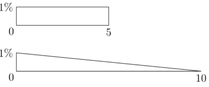
Although Value at Risk is used by the Basel Committee for determining the capi-talization that a bank needs, it turns out that VaR is insufficient for distinguishing between some kinds of different risk characteristics. The following two situations have exactly the same VaR.
0 10
1%
0 5
1%
In each case, the 95%-Value at Risk is 0. This is a great misnomer, as there are probabilities of a loss in each case. However, if we consider the notion of Maxi-mum Loss (ML) that is the measure of risk ML(X) that is defined to be the largest loss that a firm could experience with nonzero probability when that firm holds the position X (in the notation of the previous paragraph, we have that ML(X) = d), then we can observe that this measure would distinguish between the two situa-tions, as ML(X1) = 5, while ML(X2) = 10. (In this and in each of the following figures, we will adopt the notation that the first graph represents a distribution X1, while the second represents a distribution X2.) We also note that the 95%-TCE will identify that the two risk profiles are different, as 95%-TCE(X1) = 52, while 95%-TCE(X2) =R010x(1 −101x)dx =
10 3.
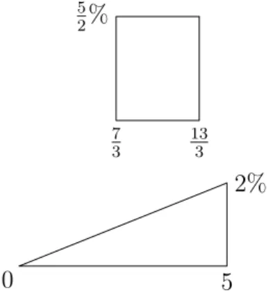
Since VaR turned out to be insufficient for our risk measuring purposes, maybe one of the two other measures is a better choice. We will start with the Tail Conditional Expectation at the 95% level. Here we look at two different situations having the same 95%-Tail Conditional Expectation.
0 5 2% 7 3 13 3 5 2%
Figure 2: Two loss distributions with equal 95%-TCEs
Both of these have the same 95%-Tail Conditional Expectation, as 95%-TCE(X1) = 95%-TCE(X2) = 103, yet there are obviously different risk patterns associated with the two loss distributions. In the first situation, there is uniform probability of loss. In the second case, the probability of loss increases as losses increase. How-ever, there is the potential for larger loss with the second situation. Each scenario might be preferable to certain institutions for specific situations, but the 95%-TCE does not alert the institution to any difference in the two different loss patterns. It is notable that both the Maximum Loss and the 95%-VaR will distinguish be-tween the two situations. 95%-VaR(X1) = 73, while 95%-VaR(X2) = 0. Likewise,
ML(X1) =133 and ML(X2) = 5.
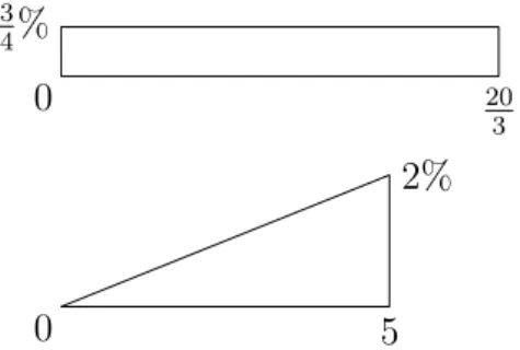
we turn to the other measure we have previously introduced - the Maximum Loss. We will again look at the last 5% of the probability distribution.
5 3 1% 4% 0 5 1%
Figure 3: Two loss distributions with equal MLs
As we see in Figure 3, the two risk models have the same Maximum Loss as both distributions have no probability occurring after the value of 5. However, there are vastly different risks involved in choosing one situation over the other. In the first case, there is a simple uniform probability of loss across all the loss levels. In the second case there is zero probability of smaller losses but a larger probability of larger losses, tapering off toward the maximum loss. Here both the 95%-VaR and the 95%-TCE will determine the difference in the two positions. We first note that 95%-VaR(X1) = 0 and that the 95%-VaR(X2) = 3. Also, the 95%-TCE(X1) = 52, while the 95%-TCE(X2) =
R5 3 x(−32x+ 17 2) = 19 5.
From these examples, we should begin to see what each of these risk measures is actually measuring. The 95% Value at Risk gives the starting point of the worst 5% of returns under the given model. The 95% Tail Conditional Expectation tells the weighted average of that worst 5% interval. And the Maximum Loss shows the worst possible loss for the given risk profile.
In order for us to obtain two distributions with the same 95%-Value at Risk, we only have to begin our figures at the same value, making sure that we have 5% of the probability after that common point. For two distributions to have the same 95%-Tail Conditional Expectation, we must have two geometric figures that have the same weighted center of mass. And for two figures to have the same Maximum Loss, we only need both to have a common point as the maximum value for which both distributions have a nonzero probability.
5.2 Insufficiency of any two risk measures
Since individual measures failed to give a thorough picture of the risk character-istics of a given risk model, maybe the situation will be better if we try using two different risk measures. Having just stated what each risk measure assesses about the risk situation, we will attempt to use measures in pairs to see if they give us a full description of the risk characteristics of a model.
We will start by using both the 95%-VaR and the 95%-TCE. Again we are left with a problem. Indeed, the two circumstances shown in Figure 4 have equal 95%-Values at Risk of 0 and equal 95%-Tail Conditional Expectations of 103, yet there are obviously different risk profiles. Again, the first model has uniform loss char-acteristics. The second has increasing probability of a larger loss, yet it does not allow for as severe of a loss as the first distribution.
Because we wanted both the 95%-VaR and the 95%-TCE to be equal, we had to meet two conditions. For the VaR condition, we needed both figures to have the same “starting point” for the greatest 5% of losses. Since the first figure is a uni-form distribution, it is easy to determine that its weighted center of mass is 103. So our second figure would have to have a weighted center of mass at103 also, which can be computed by looking at the integral calculation. One just has to choose a pdf f(x) so that (in the notation previously described) 1
.05
Rd
c x f(x) = 103. Note that
ML(X1) = 203, while ML(X2) = 5, so that the measure of Maximum Loss distin-guishes between these two distributions.
0 5 2% 0 20 3 3 4%
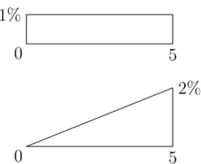
Figure 4: Two loss distributions with equal 95%-VaRs and equal 95%-TCEs Now we look at the pair of 95%-VaR and Maximum Loss, as shown in Figure 5. Once again, we are in the situation where both examples have equality of 95%-VaR, each of which is 0. And, for both distributions the Maximum Loss is 5. Yet, the risk characteristics are once again different. In the second example, there is a larger probability of larger losses, while the first example has uniform probabilities across the entire loss interval. It is notable that the 95%-TCE here will alert us to the difference in the two situations, as 95%-TCE(X1) = 52, while 95%-TCE(X2) =
10 3.
0 5 2%
0 5
1%
Figure 5: Two loss distributions with equal 95%-VaRs and equal MLs In order to produce more examples, all we would need is that both have the same starting point of the greatest 5% of losses and the same ending point of nonzero probabilities. That is, for both distributions we would need a common c and a com-mon d in the notation of the previous section. Above are two such examples that meet these criteria.
Now we will consider the circumstance of using the 95%-TCE and the ML as our risk measure pair (Figure 6). Here, the 95%-TCEs are equal, as are the MLs. Again, the risk models give different risk characteristics to those who would need to make a choice between the two. We have the uniform loss probability on a smaller interval, should we choose the first example. In the second example, the losses increase in probability as the size of losses increases.
0 5 2% 5 3 5 3 2%
Figure 6: Two loss distributions with equal 95%-TCEs and equal MLs Here, we again have two criteria that have to be met. In order for the 95%-TCEs to be equal, we need to have the same weighted centers of mass. Again, these can be determined by doing the integral calculations that were previously described. For the MLs to be equal, we again need both distributions to have the same “ending point.”
For both of the distributions we have that the 95%-TCEs are103, while the MLs are both 5. Thus, it appears from these examples that using two risk measures is not sufficient. We notice that 95%-VaR(X1) = 53, while 95%-VaR(X2) = 0, so that the third measure differentiates between the two risk profiles.
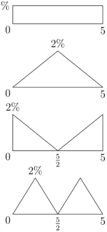
5.3 Insufficiency of all three measures
With each pair of risk measures proving insufficient to determine the entire risk loss pattern, we look to the potential that three measures might work. Our four examples in Figure 7 have equal 95%-VaRs, equal 95%-TCEs, and equal MLs, yet the risk patterns are clearly different. The first is once again a uniform loss pattern. The second example shows increasing probabilities of losses and then decreasing, while the third example does just the opposite. The fourth example shows that this pattern of increasing and then decreasing probabilities (or likewise decreasing and then increasing probabilities) could be appropriately extended to get an infinite family of examples which have equality of all three of our measures.
0 5 2 5 2% 0 5 2 5 2% 0 5 2% 0 5 1%
Figure 7: Four loss distributions with equal 95%-VaRs, 95%-TCEs and MLs In order for our examples to have equivalence of all three measures, we have to meet three criteria. We need the same “starting points” of the worst 5% of retruns
in order to make the VaRs equal. We require identical “ending points” for the MLs to be equal. Since the uniform distribution has symmetry, it will have a 95%-TCE of 52. Thus, any distribution with an equivalent 95%-TCE (and the same starting and ending points) must also be symmetric in the greatest 5% of its losses.
So our three measures do not distinguish among the potential scenarios that we might face. Obviously, something more is needed.
5.4 Extending to different probability levels
We have chosen to use the 95% level for our risk measures, but there is nothing special about the 95% level. Our examples would be just as valid if we substituted 90% or 99% or any other number in all of our measures and then scaled identically in all of the corresponding diagrams. However, this concept of considering differ-ent risk levels might also lead us to enough risk measures so that we can determine the risk profile from information about the different risk measures.
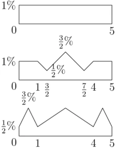
So now we will try using a vector of measures consisting of the 95%-VaR, the 99%-VaR, the 95%-TCE, 99%-TCE, and the ML. The different risk profiles demon-strated in Figure 8 are quite odd-looking, but they all have identical 95%-VaRs, 99%-VaRs, 95%-TCEs, 99%-TCEs, and MLs.
0 1 4 5 1 2% 3 2% 0 1 3 2 7 2 4 5 1% 1 2% 3 2% 0 5 1%
Figure 8: Using five risk measures
The three distributions all have the necessary geometric properties for equality of all five measures. If we wanted to form a larger family of examples with the same values for all five measures, we would need our new distributions to have the same “ending points” in order to match up the MLs. We would need them to have the same “starting points” for both the greatest 5% of losses and the greatest 1% of losses in order to have equal 95%-VaRs and equal 99%-VaRs, respectively. And we
would need symmetry in the greatest 5% of losses and in the greatest 1% of losses in order to have 95%-TCEs and 99%-TCEs, respectively, equal to the 95%-TCE and the 99%-TCE of the uniform distribution. Any figure meeting all these criteria would also be indistinguishable from the first five when viewed purely by looking at the values in our vector of five measures. Clearly several different profiles can share all five measures.
6
Discussions and Extensions
The first question that occurs to us is: how surprising should we consider these results to be? If we think of the 1−α tail as a probability distribution in and of itself (of course appropriately scaling so that we have an area of 1 rather than an area of 1−α) then we can apply theorems and facts from statistics to our situa-tion. What seems to be the most relevant to our situation is the prospect of unique determination of a probability distribution from data we know about the proba-bility distribution. It is a standard result that a probaproba-bility distribution cannot be uniquely determined from the knowledge of less than all its finite moments (i.e. from knowledge of its mean, standard deviation, skewness, kurtosis, etc. This is shown by looking at Taylor expansions for each of the moments). Thus we should expect that we cannot determine the exact risk profile for a given portfolio, even if we allow that each of the risk measures tell us something different about the risk distribution. Thus, there is reason why this result should not be completely surpris-ing to us.
We did see that it required some strange risk profiles in order for five risk measures to fail to distinguish among the risk profiles. Although our diagrams are jagged, it is an easy exercise to smooth out the corners by approximations, making sure to respect the necessary arithmetic and calculus so as not to disturb the equalities that we have honored. Using three measures tended to miss some important dis-tinctions. Although the five measure vector will miss some different risk profiles, what it misses are situations that will very rarely occur naturally. Thus, we suggest that the use of five risk measures would be appropriate for regulatory and reporting purposes.
Although it is difficult for a single risk measure to efficiently account for all the risks a bank must consider in determining its proper capital requirement, this pa-per has shown a feasible way to get a better view of these risks. In practice many different ideas have to be considered. If the five measures of risk seem unwieldy, we might consider one risk measure that is some sort of aggregation of these five measures. We also feel the need to engage in a discussion of the function(s) of risk measures. One approach might be to consider one measure for market risks and an-other for operational risks (see, for example, Embrechts, Klüppelberg and Mikosch (2007), and Guégan and Hassani (2009)). We plan to investigate the suggestions
from this paper on different data sets and present the results in a companion paper.
References
[1] Artzner P., F. Delbaen, J. Eber and D. Heath, 1997. Thinking Coherently. Risk, 10, 68-71.
[2] Basel Committee on Banking Supervision (BCBS), 1988. International conver-gence of capital measurement and capital standards, BIS, Basel, Switzerland. [3] Basel Committee on Banking Supervision (BCBS), 1996. Amendment to the
Basel Capital Accord to incorporate market Risk. BIS, Basel, Switzerland. [4] Basel Committee on Banking Supervision (BCBS), 2005. Basel II:
Interna-tional Convergence of Capital Measurement and Capital Standards: A Revised Framework, BIS, Basel, Switzerland.
[5] Bassi F., P. Embrechts, M.Kafetzaki 1996. A Survival Kit on Quantile Estima-tion, Working paper, Department of Mathematics, ETHZ, Zurich, Switzerland. [6] Caillault C., D. Guégan 2009. Forecasting VaR and Expected shortfall using
dynamical Systems : a risk Management, Frontiers in Finance, 6 (1), 26 - 50. [7] Embrechts, P., C. Klüppelberg, T. Mikosch, 2007. Modelling Extremal Events
for Insurance and Finance, Springer, Berlin.
[8] Fama E., 1965. The Behavior of Stock Markets, The Journal of Business, 38, (1), 34 - 54.
[9] Guégan D., B. Hassani, 2009. A modified Panjer algorithm for operational risk capital calculations, Journal of Operational Risks, 4 (4). 1-20.
[10] Hogg, R., S. Klugman, 1984. Loss Distributions, Wiley, New York.
[11] Mandelbrot B., 1963. The Variation of Speculative Prices, The Journal of Business, 36, (4), 394 - 414.
[12] Markowitz H., 1952. Portfolio selection, The Journal of Finance, VII, (1), 77 - 91.
[13] Rockafellar R.T., S. Uryasev, 2002. Conditional Value-at-Risk for General Loss Distributions. Journal of banking and finance, 26, 1443-1471.
[14] Stulz R.M., 1996. Rethinking Risk Management, Journal of Applied Corpo-rate Finance, (Fall), 8-24.
[15] Yamai Y., T. Yoshiba, 2002. Comparative Analyses of Expected Shortfall and Value-at-Risk : Their Validity under Market Stress, Monetary and Economic Studies, Bank of Japan, 20, 181-238.