HAL Id: halshs-00270295
https://halshs.archives-ouvertes.fr/halshs-00270295
Submitted on 4 Apr 2008
HAL is a multi-disciplinary open access archive for the deposit and dissemination of sci-entific research documents, whether they are pub-lished or not. The documents may come from
L’archive ouverte pluridisciplinaire HAL, est destinée au dépôt et à la diffusion de documents scientifiques de niveau recherche, publiés ou non, émanant des établissements d’enseignement et de
A Quantitative Evaluation of Payroll Tax Subsidies For
Low-Wage Workers: An Equilibrium Search Approach
Arnaud Chéron, Jean-Olivier Hairault, François Langot
To cite this version:
Arnaud Chéron, Jean-Olivier Hairault, François Langot. A Quantitative Evaluation of Payroll Tax Subsidies For Low-Wage Workers: An Equilibrium Search Approach. Journal of Public Economics, Elsevier, 2008, 92 (3-4), pp.817-843. �10.1016/j.jpubeco.2007.09.012�. �halshs-00270295�
A Quantitative Evaluation of Payroll Tax
Subsidies For Low-Wage Workers :
An Equilibrium Search Approach
Arnaud Ch´
eron
EDHEC & GAINS (Universit´e du Maine)
acheron@univ-lemans.fr
Jean-Olivier Hairault
Paris School of Economics & Universit´e Paris 1 & IZA
joh@univ-paris1.fr
Franc
¸ois Langot
∗Paris School of Economics & GAINS (Universit´e du Maine) & IZA
flangot@univ-lemans.fr
June 5, 2007
∗Address: PSE, 48 boulevard Jourdan, 75014 Paris. The authors acknowledge financial
support from the French Ministry of Labor. We benefited from fruitful discussions with S. Gilchrist, P.Y. H´enin, J.M Robin and F. Postel-Vinay. We thank seminar participants at the SED meeting (Paris, 2003), T2M (Orl´eans, 2004), SCSE congress (Qu´ebec, 2004), Fourgeaud seminar (Paris, 2003), PSE-Jourdan seminar (Paris, 2004) and the CREST seminar (Paris, 2004). We thank two anonymous referees for helpful comments. We are specially indebted to Pierre-Yves Steunou for excellent research assistance. Any errors and omissions are ours.
Abstract
Phelps (1994) presented the case for a low-wage subsidy policy. Since the mid-1990s, France has experimented with this strategy. This paper evaluates the effect of this policy on employment and also on output and welfare. We construct an equilibrium search model incor-porating wage posting and specific human capital investment, where unemployment and the distribution of both wages and productivity are endogenous. We estimate this model using French data. Numeri-cal simulations show that the prevailing minimum wage allows a high production level to be reached by increasing training investment, even though the optimal minimum wage is lower. We show that payroll tax subsidies enhance welfare more than a reduction in the minimum wage when they are spread over a large range of wages in order to avoid specialization in low productivity jobs.
JEL codes : C51, J24, J31, J38
Keywords: Employment, productivity, equilibrium search, labor costs
Introduction
High labor costs typically are considered the primary cause for high unem-ployment levels in continental European countries (see Blanchard and Wolfers (2000)) where the welfare state has put in place high payroll taxes and min-imum wages. Despite a lack of formal evidence evaluating this claim (Katz (1996)), Phelps (1994) presented a case for a low-wage employment subsidy policy as a means to reduce the unemployment of such workers. Phelps (1994) proposed “a system of low-wage employment subsidies be introduced, a subsidy to every qualifying firm based on the stock of low-wage workers on its roll” (p. 56, Phelps (1994)). This policy differs from most of the prevail-ing subsidy policies1: for instance, the Targeted Jobs Tax Credit in effect in
the US during all of the 1979 to 1994 period concerned hirings, as in most developed countries. However, France had already implemented the original strategy, which consists of a high minimum wage2 compensated for by large,
permanent payroll tax subsidies on low wage employment. It must be noted that the UK, the Netherlands and Belgium, have also experimented with such permanent subsidies for disadvantaged workers, but to a lesser extent than in France.
In this paper, we use French data to evaluate the performance of this wage subsidy policy suggested by Phelps (1994). Relative to a minimum wage reduction policy, a wage subsidy implies a budgetary cost, but it may preserve the welfare of the low-wage workers. On the other hand, this labor cost-reducing policy may be implemented with two different options for a given budgetary cost: either it concentrates subsidies at the minimum wage or it spreads them over a large range of wages. The former clearly aims at dampening the negative effect on employment of the minimum wage, but risks introducing severe distortions. For instance, Katz (1996) emphasizes the risk of stigmatization against a narrowly targeted population of workers which could explain the low employment impact of subsidy policies. In this paper, as firms are likely to respond to wage subsidies by increasing their utilization of workers in the targeted population, we focus on the risk of dis-tortion in job allocations and its implication in terms of productivity. While several econometric papers have already highlighted the positive impact of
1
A wage subsidy can be applied to all employment, to net changes in employment or to new hires.
2
France has the highest minimum wage/average wage ratio (known as the Kaitz ratio) in Europe: it is equal to 55%, whereas all the other European countries have a ratio lower than 50%. Research on the French labor market has pointed out extensively the negative role played by the minimum wage legislation due to increasing labor costs (for instance Laroque and Salani´e (2000) and (2002)).
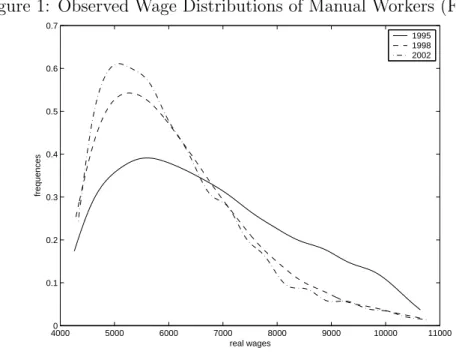
this policy on employment in France (for example, Kramarz and Philippon (2001) and Cr´epon and Desplatz (2002)), Malinvaud (1998), however, stresses a potential negative impact on productivity due to a bias in job creation at the bottom of the wage distribution. When the wage distribution is strongly interrelated with the productivity distribution, payroll tax subsidies could shrink productivity, which in turn could dampen output. Figure 1 shows a higher concentration at the bottom of the wage distribution of manual work-ers after the setting up in 1995 of the subsidy policy.3 Crepon and Desplatz
(2002) also provide some empirical evidences on the decrease of productivity.
Figure 1: Observed Wage Distributions of Manual Workers (France)
40000 5000 6000 7000 8000 9000 10000 11000 0.1 0.2 0.3 0.4 0.5 0.6 0.7 real wages frequences 1995 1998 2002
In this paper, we propose a wage posting model with specific human capital investments and a bilateral endogenous search including on-the-job search, in the line of Mortensen (2000). This framework generates wage and productivity distributions and an equilibrium unemployment rate that are consistent with the data4. In our framework, the expected job duration,
3
We retain only full-time manual workers from the Labor Force Survey (“Enquˆete emploi”) provided by the Institut National de la Statistique et des Etudes Economiques (INSEE), as in the empirical part of our study. We estimate the wage distribution using a wage set of N ∈ [14, 100; 14, 400] individuals: the size of this vector (N) varies every year, but the difference is not significant.
4
In our model, as is usual in equilibrium search models, the probability of job-to-job transitions declines as one moves up the wage distribution. Yet, Bowlus and Neumann (2004) provide some empirical evidence against this prediction based on the existence of negative wage changes for high wage workers. By focusing on low-skilled workers, we avoid
which depends on the degree of labor market tightness, determines the extent to which firms invest in specific human capital. Beyond a pure distribution effect due to the policy bias towards the low-paid workers, productivity could also be decreased by less investment in specific human capital from firms because lower labor costs reduce the expected job duration. Our model leads to a joint theory of wages, productivity and employment, where the effect of labor market institutions such as the minimum wage are not determined a priori by job creation disincentives or the reduction of the monopsony power of firms. Moreover, contrary to Flinn and Mabli (2006), the average job-search efficiency is not necessarily improved when unemployment increases. By allowing for the existence of transition periods between short-term and long-term unemployment, the average job-search efficiency of unemployed workers varies with the endogenous ratio of short-term unemployment to long-term unemployment. This ratio depends on the number of vacancies, which is in turn influenced by the average job-search efficiency. This creates a potential interplay between labor supply and labor demand which we view as necessary to identify the overall impact of a decrease in labor costs.
We therefore propose a structural model of the French low-skilled workers labor market that enables us to evaluate quantitatively the employment and productivity effects of the French labor cost reducing policy. This structural strategy differs from recent econometric exercises (see for instance Kramarz and Philippon (2001) or Cr´epon and Desplatz (2002)). It also allows us to conduct counterfactual policy experiments, and, in particular, study the optimal range of wage levels that should be covered by such subsidies. In contrast to the equilibrium search literature which seeks to match the existing stationary wage distribution (Ridder and Van den Berg (1998), Bontemps, Robin, and van den Berg (1999) and Postel-Vinay and Robin (2002)), we propose an equilibrium search model that is also suitable for policy analysis. The equilibrium search literature traditionally proposes a theory of wage distribution consistent with the labor market equilibrium. Even if firms and workers are ex-ante identical, Burdett and Mortensen (1998) show that there is a dispersed equilibrium wage distribution due to the existence of job-to-job transitions. From an empirical point of view, Ridder and Van den Berg (1998) Bontemps, Robin, and van den Berg (1999), or Postel-Vinay and Robin (2002) show that it is necessary to add an exogenous productivity distribution in order to match the observed data. Nevertheless, despite its empirical performance, this framework has been rarely used to conduct pol-icy evaluations. The notable exception is Ridder and Van den Berg (1998). With exogenous heterogeneity in productivity, a decrease in the minimum this problem.
wage makes additional productivity segments profitable and increases the number of firms in the economy. Due to composition effects, labor cost changes influence average productivity. However, in models with exogenous productivity, the productivity level in any firm is given, which limits the ef-fect on average productivity. On the other hand, the labor demand side in this literature is not well-suited to policy analysis as the firms’ hirings do not depend on labor costs. Flinn (2006) extends the equilibrium search approach in this direction by considering a stochastic matching model with Nash bar-gaining. Flinn (2006) assumes an exogenous productivity distribution, does not allow on-the-job search however, thus restricting search to unemployed workers along the lines of Albrecht and Axell (1984) and Eckstein and Wolpin (1990).
Our modeling strategy relies on three key assumptions: the wage post-ing hypothesis, the absence of counter-offers and the fact that productivity is governed by specific human capital investments.5 Manning (1993) argues
that bargaining cost considerations make the wage setting assumption not restrictive for anonymous markets with low-skilled workers. While Shimer (2006) points out that the equilibrium wage distribution is no longer unique in wage bargaining models with on-the-job search, Cahuc, Postel-Vinay, and Robin (2006) show that the introduction of renegotiation circumvents the multiple equilibria outcome. Moreover, they estimate that the bargaining power of the unskilled workers is small: the wage posting assumption cannot be rejected. Our assumption regarding the absence of counter-offers6 is
mo-tivated by Postel-Vinay and Robin (2004) who argue that it is optimal for low productive firms not to commit to matching outside wage offers7.
Con-cerning the third assumption, the specific human capital, Postel-Vinay and Robin (2002) show that the productivity differential across firms explains about half of the French low-skilled wage variance. The remaining part is due entirely to search friction, leaving no room for individual fixed effects. We interpret this as the absence of a significant general human capital effect for the low-skilled workers8. We also exclude physical capital from the
analy-5
These points receive some support in Manning (2003).
6
See also the (Mortensen 2003) criticism of counter-offers endorsed by Shimer (2006): “unlike in the market for academic economists in the United States, making counteroffers is not the norm in many labor markets”.
7
This avoids the moral hazard problem created by workers who prefer to search more intensively knowing that outside offers lead to wage increases.
8
This is consistent with previous empirical microevidence along the lines of Lynch (1992) and Black and Lynch (1996) who stress the significant role of specific firms’ in-vestments in human capital in the distribution of workers’ wages and productivity. Inter-national evidence shows that the returns of firm-provided training are significant: 2% in Germany (see Pischke (1996)) and 12% in the US (Blanchflower and Lynch (1994)).
sis: Robin and Roux (2002) show that the introduction of physical capital in a model `a la Burdett and Mortensen does not help match the observed French wage distribution. Hence, we assume that the firms’ heterogeneity observed in the data comes only from their various investments in specific human capital.
A key implication of our theoretical framework is that the wage distrib-ution will not display a point mass at the minimum wage. As can be seen from Figure 1, this implication is validated on French data if one considers only full-time workers (see also Postel-Vinay and Robin (2002))9. In
con-trast, Dares (2006) documents that part-time workers do exhibits a point mass at the minimum wage. While such workers account for 40% of the den-sity at the minimum wage, taking into account these part time jobs would have introduced too many complexities and heterogeneities into our theo-retical framework. Moreover, part-time jobs in France benefit from specific policy arrangements, especially concerning the subsidy policy in question. We therefore prefer to focus on a consistent worker population.
We estimate key parameters of the model on French data using an in-direct inference method. Based on statistical tests, we cannot reject the hypothesis that the theoretical wage distribution is generated by the same law as the observed one. In particular, because the productivity distribu-tion plays a central role in the replicadistribu-tion of the observed wage density, it provides a powerful identification strategy to estimate the elasticity of pro-ductivity relative to human capital investment. We show that this model is able to better replicate the deformation of the wage distribution following the low-wage subsidy policy than a traditional equilibrium search model with exogenous productivity. Thus, while search models based on exogenous pro-ductivity differences can replicate existing wage distribution, they are unable to explain variations in such distributions owing to policy changes. This is a key result which strongly supports the need to adopt a framework with endogenous human capital investments when considering the impact of labor cost-reducing policies.
Taking into account a costly human capital investment creates a potential trade-off between employment and productivity. The investment channel competes with the employment channel to determine the output effect of the labor cost-reduction policies. As a benchmark case, we investigate the various implications of a minimum wage change on output. The optimal level for a
9
This question is a disputable empirical issue. Ridder and Van den Berg (1998) do not observe a spike at the minimum wage when estimating the wage densities on Dutch data. DiNardo, Fortin, and Lemieux (1996) find that spikes are more prevalent for females than for males in the US. On the contrary, Flinn (2006) favors the view that there is a spike in the US.
minimum wage seems to be slightly lower (by 12%) than the existing one: a decrease in the minimum wage leads to an employment boost, partially compensated by a decline in labor productivity. The investment channel explains why the optimal minimum wage is relatively high which contrasts with the result of Ridder and Van den Berg (1998) and to a lesser extent of Flinn (2006).
We then evaluate the performance of the subsidy policy. Given that the goal of the payroll tax subsidies is to reduce labor costs (without removing the minimum wage legislation), we show that this policy leads to an employ-ment boost which is offset in part by a deterioration in productivity. We show that the current implementation of this policy in France is close to be optimal owing to the fact that subsidies are allocated over a broad range of wages and not only at the minimum wage level. Removing the investment channel from the analysis leads to an opposite recommendation, namely to concentrate exemptions at the minimum wage level. Our results thus imply that the French policy of labor subsidies provides an efficient way of concili-ating a higher employment level with maintaining the welfare of the low-wage workers.
This paper is organized in three sections. Section 1 is devoted to the presentation of the theoretical model. Section 2 presents the calibration and empirical performances of the model. Quantitative results for different policy experiments are discussed in Section 3.
1
The Theoretical Model
Our theoretical framework is based on the Mortensen (2000) equilibrium search model with wage posting and training investment by firms. This framework is extended in three ways. First, we take into account the transi-tion between short- and long-term unemployment.10 Secondly, we introduce
heterogeneity in the search intensity of employees and short- and long-term unemployed workers11. Finally, we incorporate the minimum wage
legisla-tion.
10
See Albrecht and Vroman (2001) for a Pissarides (1990) style of matching model where the heterogeneity of the reservation wages is due to the exclusion of some unemployed workers from the unemployment benefit system. From an empirical point of view, half of unemployed individuals are not eligible for the French unemployment benefit system, but we qualify them as long-term unemployed for simplicity.
11
As we focus on firms’ policies on wages and specific human capital investment (i.e. hiring decisions), we do not introduce an endogenous search effort, contrary to Christensen, Lentz, Mortensen, Neumann, and Werwatz (2005).
The total labor force is composed of employed workers, unemployed work-ers entitled to unemployment benefits and unemployed workwork-ers excluded from the compensation system but entitled to a minimum income. We assume that these three components of the total labor force are not perfectly equivalent in the matching process. An employed worker accepts any offer in excess of the wage currently earned. Yet, all unemployed workers will accept the first offer that is higher than the common reservation wage of their sub-group. Differ-ences in unemployment benefit compensation levels and the intensity of the job search process generate two distinct reservation wages in the economy.
Firms create “job sites” and each job is either vacant or filled. The equilibrium level of vacancies is endogenously determined by a free entry condition. For each job vacancy, firms also determine the associated wage and firm-specific training offered.
In the remainder of this section, we begin by presenting the conditions that characterize the equilibrium flows for the two unemployed worker pop-ulations and for each job relative to a given wage of the distribution. Then, we determine the reservation wages through the derivation of the optimal behavior of workers. Based on the firm’s optimal decisions, we derive the vacancy rate, the wage offer distribution and the human capital investment distribution.
1.1
Labor Market Flows
1.1.1 Matching Technology
According to Pissarides (1990), the aggregate number of hirings, H, is deter-mined by a conventional constant returns to scale matching technology:
H = h(v, hee + hsus+ hlul)
where v is the number of vacancies, he ≥ 0, hs ≥ 0, hl ≥ 0 are the
exoge-nous search efficiencies (intensities) for employed workers and short-term and long-term unemployed workers, represented (in number) by e, us and ul,
re-spectively. We normalize e + us+ ul to 1 and we denote u ≡ us + ul and
h = hee + hsus+ hlul.
If we set θ = v
h as labor market tightness, the arrival rates of wage offers
for workers are :
• for the employees
heλ(θ) ≡ h e h H e + us+ ul = h eH h
• for the short-term unemployed hsλ(θ) ≡ h s h H e + us+ ul = h sH h • for the long-term unemployed
hlλ(θ)≡ h l h H e + us+ ul = h lH h
Accordingly, the average duration of a spell before a wage offer contact is 1/(heλ(θ)) for the employees, 1/(hsλ(θ)) for the short-term unemployed and
1/(hlλ(θ)) for the long-term unemployed.
The transition rate at which vacant jobs are filled is:
q(θ) = H v = h µ 1,h v 
The average vacancy duration is thus 1/q(θ).
1.1.2 Entries and Exits from Unemployment
Let xsand xl denote the endogenous reservation wages of the short-term and
long-term unemployed, respectively. The steady state level of short-term unemployment (us) is derived from the following equilibrium flows:
s(1− u) | {z } = h sλ(θ) [1 − F (xs)] us | {z } + δu s |{z} firings hirings flow into
long-term unemployment
where s ∈ [0, 1] is the exogenous job destruction rate, F (w) denotes the distribution function of wage offers w and δ ∈ [0, 1] is the probability of short-term unemployed workers transitioning to long-term unemployment. When δ is allowed to depend on the elapsed duration of unemployment, the model becomes non-stationary. For simplicity, we assume stationarity with δ constant as in Albrecht and Vroman (2001). The steady state level of long-term unemployment (ul) is given by:
δus
|{z} = hlλ(θ) [1− F (xl)] ul
| {z }
flow out of hirings short-term
These equations show that the fraction of long-term unemployed in the total unemployed population (ul/u) decreases with the tightness of the
la-bor market (θ): when θ increases, the expected duration of unemployment decreases, as does the probability of becoming long-term unemployed.
1.1.3 Entries and Exits from Employment at or Less than Wage w
Let G(w) denote the fraction of workers employed at or less than wage w. This function is derived from the following equilibrium flows:
• If xl≤ w < xs, (1− u)G(w)heλ(θ) [1 − F (w)] | {z } + s(1| − u)G(w){z } = h lλ(θ)F (w)ul | {z } volontary quits firings hirings
• If w ≥ xs,
heλ(θ) [1− F (w)] (1 − u)G(w)
| {z } + s(1| − u)G(w){z } volontary quits firings = ushsλ(θ)F (w) + ulhlλ(θ)F (w) | {z } − u s hsλ(θ)F (xs) | {z } potential rejections hirings
1.2
Behaviors
1.2.1 WorkersThe total income of workers is composed of labor market earnings and trans-fers (government budget surplus and firms’ profits12) which are uniformly
distributed across households denoted by T . Let Vn(w) denote the value
function for an employed worker who earns w, Vus the value function for
a short-term unemployed person who is paid b unemployment benefits and Vul the value function of a long-term unemployed individual who is paid a
minimum social income msi. These functions are solved by:
rVn(w) = u((1− tw)w +T ) + heλ(θ) Z w [Vn( ˜w)− Vn (w)] dF ( ˜w)− s [Vn (w)− Vus ] rVus = u(b + T ) + hsλ(θ) Z xs [Vn( ˜w) − Vus] dF ( ˜w) − δ£Vus − Vul¤ 12
rVul = u(msi + T ) + hlλ(θ) Z xl £ Vn( ˜w) − Vul¤dF ( ˜w)
where r ≥ 0 and tw ∈ [0, 1] stand for the real interest rate and employees’
payroll taxes, respectively. The utility function u(·) is assumed to be a Con-stant Relative Risk Aversion (CRRA) and takes into account risk aversion in the determination of the reservation wage. The reservation wage policies xs
and xl are derived from the two conditions Vn(xs) = Vus and Vn(xl) = Vul.
1.2.2 Firms
Let k be the match specific investment per worker and f (k) the value of worker productivity which is an increasing concave function of this invest-ment. It is assumed that whenever an employed worker finds a job paying more than w (voluntary quit), then the employer seeks another worker. When an exogenous quit (destruction) occurs, the job receives no value. Hence, the expected present value of the employer’s future flow of quasi-rent once a worker is hired at wage w stated as J(w, k), solves:
rJ(w, k) = f (k)− (1 + tf(w))w− heλ(θ)[1− F (w)][J(w, k) − V ] − sJ(w, k)
where tf(w)≥ 0 is the employer’s payroll taxes. This tax can be a function
of the wage when employment subsidies are introduced.
In turn, the asset value of a vacant job solves the continuous time Bellman equation:
rV = max
w≥xl,k≥0{η(w) [J(w, k) − p
kk− V ] − γ}
where γ is the recruiting cost, pk stands for the relative price of one unit of
human capital, and η(w) is the probability that a vacancy with posted wage w is filled. This probability is defined by:
η(w) = P rob(e|u l)ul v + P rob(e|us)us v + P rob(e|e)(1 − u) v
where the first, second and third term shows the acceptance rate of a job offer, respectively, for a long-term unemployed person, a short-term unemployed worker and an employed worker. These probabilities are:
P rob(e|ul) = hlH h if w≥ xl P rob(e|us) = ½ hs H h if w≥ xs 0 if w < xs P rob(e|e) = heH hG(w)
where G(w) is the fraction of employed workers with earnings equal to or less than w. The probability functions of the reservation wages are given by:
η(w) = H v · hl hu l+ h e h(1− u)G(w) ¸ ∀ w ∈ [xl, xs] η(w) = H v · hl hu l+ h s hu s+h e h(1− u)G(w) ¸ ∀ w ∈ [xs, w]
where H/v = λ(θ)/θ gives the probability of having a contact with a firm. Free entry conditions at each wage level imply that V = 0 and expected intertemporal profits are identical for w ≥ w, where w is the lowest wage level offered. Actually, xl≤ w, because it is not in the firms’ interest to offer
a wage rejected by all workers. Hence, labor market tightness θ, the wage distribution function F (w) and firms’ investment in human capital k(w) can be derived from the system of equations defined by:
γ = η(w) · max k≥0{J(w, k) − pkk} ¸ ∀w ≥ w (1) with F (w) = 0. Employers have two reasons for offering a wage greater than w. First, the firm’s acceptance rate (η(w)) increases with the wage offer, since a higher wage is more attractive. Second, the firm’s retention rate increases with the wage paid by limiting voluntary quits that lead to an increase in J(w, k). The wage strategy implemented by firms is strongly interrelated with human capital investment decisions.
As each employer pre-commits to both the wage offered and the specific capital investment in the match, it is easy to show that the optimal invest-ment solves:
f′
(k) = pk(r + s + heλ(θ)[1− F (w)]) =⇒ k = k(w) ∀w ≥ w (2)
Therefore, the level of specific human capital increases with the level of the wage offer. Indeed, a higher wage reduces the probability that an employee will accept job offers from other firms. The negative relationship between wage and labor turnover creates incentives to train employees. When the wage is high, the expected duration of the match is longer and the period during which the firm can recoup its investment increases. Therefore, firm-specific productivity increases with wages.
1.3
Labor Market Equilibrium
Assumptions on Production Technology
We assume that the production function satisfies the following restrictions: f′(0) =
Equilibrium Definition and Properties
A steady state search matching equilibrium defines a reservation wage policy, {xs, xl}, a vacancy rate (v = θh), a long-term unemployment rate ul, a
short-term unemployment rate uc, a wage offer distribution F (w) and a specific
human capital investment function k(w). Appendix A presents the system of equations to solve this equilibrium in more detail.
Proposition 1 There is only one strictly positive level of vacancy rate.
See Appendix B.1 for the formal proof of this proposition, which extends Mortensen (2000)’s work.
Proposition 2 There is a wage interval [wl, xs[ over which there
is no wage offer.
Appendix B.2 shows a detailed proof. This equilibrium property suggests that, over [wl, xs[, the increase in temporary profits associated with a decrease
in wages does not compensate for the loss due to higher rotation costs in the long-term unemployed worker segment.
Corollary If wl > xl, then the support of the wage distribution
is formed by two subsets[xl, wl]∪[xs, w]. Otherwise, all posted wages
are included in the set [xs, w].
This suggests that, if wl < xl, the increase in temporary profits when
offering a wage lower than xs is never compensated by the loss due to higher
rotation costs.
The introduction of hiring costs implies that ex ante identical firms have the same strictly positive expected profits. As shown in Quercioli (2005), this ensures a unique wage offer distribution with no atoms.13 The proofs
provided in Appendix B are satisfied for all payroll tax rules.
The Incidence of a Minimum Wage
The introduction of a minimum wage (mw) may affect the properties of the equilibrium in the following ways:
• If the minimum wage is lower than xl, it is not a constraint;
• If the minimum wage is greater than xs, its value is the lower posted
wage: w = mw;
13
Without hiring costs, the expected equilibrium profit could be equal to zero. In this case, Quercioli (2005) shows that multiple equilibria can occur.
• If the minimum wage is included in ]xl, wl[ then w = mw;
• If the minimum wage is included in ]wl, xs[, then w = xs; or
• If wl < xl then w = max{xs, mw}.
1.4
Efficiency
To evaluate the impact of labor market policies on the equilibrium, we first focus on the steady state aggregate output flow net of the recruiting costs, as defined by: Y = (1− u) | {z } Z w w f (k(w))dG(w) | {z } − γv |{z} Employment (E)× Productivity (P)
| {z } Hiring costs gross output − pkhsλ(θ)us Z w w k(w)dF (w) | {z } − pkhlλ(θ)ul Z w w k(w)dF (w) | {z }
training costs training costs short-term unemployed long-term unemployed − pkheλ(θ)(1− u) Z w w µZ w w k(w)dF (w) ¶ dG(w) | {z } training costs job-to-job mobility
Average productivity P may vary in the model due to a distribution effect dG(w), but also because of less investment k(w) from firms in specific human capital for any wages w. In models with exogenous productivity, the productivity level in any firm is given, which limits the effect on average productivity to a pure distribution effect.
Taking into account a costly human capital investment creates a poten-tial trade-off between employment and productivity. The higher the labor market tension, the higher the employment. The increase in the probabilities of a firm contacting a worker increases hirings as in a traditional matching model, but, by increasing job-to-job transitions, this leads to two antago-nistic effects on average productivity. More job-to-job transitions tend to concentrate the earnings distribution more to the right, increasing the pro-ductivity by a pure distribution effect. Hereafter we refer to a job-to-job
transition effect. However, as the expected job duration decreases, the re-turn on the human capital investments diminishes, leading to a decrease in the average productivity by an “investment effect”. Let us emphasize that this investment effect, not only impacts on the level of capital, but also on its distribution, as the capital decreases more at the bottom of the job dis-tribution where firms particularly fear job turnover. These two effects will compete with employment variations to determine the output impact of the labor cost-reduction policies examined in the next section.
We also compute aggregate welfare, which takes into account the risk aversion of workers and the distributive implications of different reforms. Here, we plan to capture the variations in the relative situation of workers and their impact on aggregate welfare for a degree of concavity given by the utility function u: W = (1 − u) µZ w w Vn(w)dG(w) ¶ + usVus+ ulVul
This implies the need to determine the variations in the government budget surplus (B) and firms’ profits (Π) as well as the way they are distributed across households. We assume that they are uniformly redistributed via lump-sum transfers across all agents so as to not interfere with the direct distributive effects of policy reforms. As the size of the population is normal-ized to one, the instantaneous utility functions are u((1− tw)w +T ) for the
employed workers, u(b+T ) for the short-term unemployed and u(msi+T ) for the long-term unemployed, where total transfersT are defined by T = B+Π. More precisely, the budget surplus is defined by:
B = (1 − u) µZ w w [tf(w) + tw]wdG(w) ¶ − (us × b + ul × msi) Aggregate firms’ profits are defined by:
Π =Y − (1 − u) µZ w w [1 + tf(w)]wdG(w) ¶ .
2
Estimation and Test of the Model
This section describes the econometric method we used to estimate the struc-tural parameters of the model. Because strucstruc-tural econometric models are sensitive to misspecification, we choose an empirical strategy which ensures robust estimates of the unknown parameters. As the likelihood function can-not be derived analytically, it can be replaced by either an approximation
of the exact function (see Bontemps, Robin, and van den Berg (1999) or Rosholm and Svarer (2004)) or by the exact likelihood function of an ap-proximated model (Gouri´eroux and Monfort (1994)). We choose the latter strategy and, more specifically, the indirect inference method, which allows us to run a simple global specification test of our model.14 The benefit derived
from testing the model, however, comes at the cost of making parametric assumptions.
2.1
Estimation method
The indirect inference method consists of replacing the computation of an-alytic moments with simulations. The moments underlying the estimation are based on wage distributions. We focus on a sub-sample of full-time man-ual workers, who are affected by the minimum wage and the probability of being excluded from the unemployment benefit system. This enables us to detect the dimensions along which our simple structural model is capable of mimicking a set of moment restrictions.
The vector Φ (dim(Φ) = 17) contains all the parameters of the model: Φ ={he, hs, hl, ζ, γ, s, δ, σ, b, msi, r, t
w, tf, pk, α, A, A1}
where the parameters {α, A, A1} characterize the production function such
that f (k) = A1+ (k + A)α. We choose this particular production function to
simplify the estimation procedure. Indeed, it implies that a worker without training has a strictly positive inherited productivity. We choose a value of A such that k(xc) = 015.
The parameter σ denotes the risk aversion of the workers: u(x) = x1−σ
1−σ.
Finally, the parameter ζ denotes the elasticity of the matching function H = vζ(hee + hsus+ hlul)1−ζ.
We restrict the size of the vector of unknown structural parameters: Θ ={α, pk, he}
The absence of empirical evidence for these key parameters of the model motivates this choice. The estimation of the vector Θ is conducted under the following set of restrictions:
• A first vector Φ1, with dim(Φ1) = 7, defined by
Φ1 ={s, δ, σ, msi, r, tw, tf}
14
See Gouri´eroux, Monfort, and Renault (1993) or Gouri´eroux and Monfort (1994) for a general presentation of these methods. See Collard, Feve, Langot, and Perraudin (2002) for an applied study.
15
is fixed on the basis of external information.
1. The destruction rate s comes from Cohen, Lefranc, and Saint-Paul (1997): s = 0.0185.
2. The parameter δ is chosen so that the average short-term unem-ployment spell corresponds to the benefit duration, i.e. 30 months, (δ = 1/30).
3. Microdata suggest that σ = 2.5 is an admissible value (see At-tanasio, Banks, Meghir, and Weber (1999)).
4. The minimum income msi is fixed at its 1995 institutional value: FF 2,500 (French Francs, FF hereafter).
5. The annual interest rate is fixed at 4%.
6. Payroll taxes on labor tf and tw for firms16 and workers are set
at, respectively, 40% and 20%.
• The second vector Φ2, with dim(Φ2) = 6, defined by
Φ2 ={b, hs, hl, A1, γ, ζ}
is calibrated, using the model restrictions, to reproduce some stylized facts and assumptions:
1. The unemployment replacement rate (b/E(w)) is fixed at 0.6, ac-cording to Martin (1996).
2. The unemployment rate u equals 15.51%.
3. The ratio of long-term to short-term unemployed workers ul/u is
45.75%.
4. The condition of free entry in the labor market is respected (no sunk costs linked to the creation of a vacancy).
5. Hiring costs γθ/λ(θ) equal 0.3 as in Mortensen (2003). These costs correspond approximately to 2.5% of wages (Abowd and Kramarz (1998)).
6. The minimum wage is fixed at a level consistent with the historical French experience (see CSERC (1999)). For a one percent fall in the minimum wage, 14,000 jobs are created. This leads to a value of ζ equal to 0.21.
16
Given the set of moments, calibrated parameters and policy functions, the estimation method is conducted as follows:
Step 1: The vector of moments ψ is estimated by minimizing the following loss function:
QN = hN(wi; ψN)′ΩNhN(wi; ψN)
where ΩN is a positive definite weighting matrix and N denotes the size of
the sample. {wi}′ represents the s-dimensional set of wages paid to each
manual worker i in the 1995 set of observed random variables. The choice of ψ moments is a critical step in the estimation method, but it is not driven by the model’s specification. Rather, it should encompass as many data features as possible to avoid an arbitrary choice and reduce estimation biases. Therefore, we choose a set of moments that fully explain wage densities. In our case, h(.) takes the form
h(wi; ψ) = E wi− µ (1[wi<D1]wi− µ1) (1[Dn≤wi<Dn+1]wi − µn+1) (1[D8≤wi<D9]wi− µ9) for n = 1, .., 7
where Dn denotes the wage deciles n = 1, ..., 9. The estimated moment µ is the average wage in the sample, and µn is the average wage between the Dn
and Dn + 1 deciles. This minimal set of moments allows us to capture the shape of the observed wage density.
Step 2: Given the vector of structural parameters Θ, the simulated wage density is computed from the set of equations defining the theoretical model.
Step 3: An estimate bΘ for Θ minimizes the quadratic form: J(Θ) = g′ NWNgN where gN = ³ b ψN − eψN(Θ) ´
, WN is a symmetric non-negative matrix defining
the metric, bψN is the vector of the estimated moments {µ, µ1, ..., µ9}, and
e
ψN(Θ) denotes the set of moments implied by the model simulations.
Steps 2 and 3 are conducted until convergence i.e. until a value of Θ minimizing the objective function is obtained.17
17
The minimization of the simulated criterion function is carried out using a Nelder-Meade minimization method provided in the Optim matlab numerical optimization tool-box. At convergence of the Nelder-Meade method, a local gradient search method was used to check convergence.
A preliminary consistent estimate of the weighting matrix WN is required
for the computation of bΘN. It can be based directly on actual data and, here,
corresponds to the inverse of the covariance matrix of √N ( bψN − ψ0), which
is obtained from Step 1.
For the purpose of identification, we impose the condition that the number of moments exceeds the number of structural parameters. Thereby, we can conduct a global specification test along the lines of Hansen (1982), such that J− stat = NJ(Θ), which is asymptotically distributed as a chi-square, with a degree of freedom equal to the number of over-identifying restrictions.
Beyond these traditional statistical tests, we use a simple diagnostic test that locates the potential failures of the structural model. Each element of gN
measures the discrepancy between the moments computed from the data and those computed from model simulations. A small value for a given element in gN indicates that the structural model is able to account for this specific
feature of the data, while large values may reveal some failures. Collard, Feve, Langot, and Perraudin (2002) show that a statistic measuring the gap with a particular moment and its simulated counterpart, denoted “Diag. Test”, is asymptotically distributed as a N (0; 1).
2.2
The Empirical Performances of the Model.
We use data from the 1995 French Labor Force Survey (“Enquˆete emploi”). We consider this year which precedes large structural reforms of the French labor market and retain only full-time manual workers. Thus, in this partic-ular case, {wi} consists of the wage set over N = 14202 individuals. Wages,
minimum income and unemployment benefits are expressed in 1990 French Francs (FF).
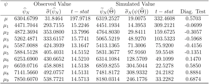
Table 1 reports estimates for the structural parameters and the global specification test statistic (J−stat). The model is not globally rejected by the data, as the P-value associated with the J−stat is 97.65%. A second feature that emerges from Table 1 is that all structural parameters are estimated with precision. In the following paragraph, we discuss the model implications for this set of parameter estimates.
In the step following the global specification test, we check the struc-tural model’s ability to reproduce empirical moments. We obtain observed and simulated values of moments (Table 2). First, all observed moments are significant so that this set of historical moments is a sufficient table of experience to test our model. Secondly, Table 2 shows that the simulated moments are also estimated with precision.18 In addition, they match their
18
Table 1: Parameter Estimates Θ Θb bσ(Θ) t− stat α 0.7158 0.0310 23.0790 pk 18.2866 1.2814 14.2706 he 0.5265 0.0147 35.7266 J − stat 1.6519 P-value 97.65%
empirical counterparts relatively well: the diagnostic test (Diag. Test) does not lead to rejection of the model in terms of its ability to reproduce each moment.
Table 2: Estimated Moments for Simulated and Observed Data
ψ Observed Value Simulated Value b
ψN σ( bb ψN) t− stat ψeN( bΘ) eσN(ψ( bΘ)) t− stat Diag. Test
µ 6304.6799 31.8464 197.9718 6319.2527 19.0075 332.4608 0.5703 µ1 4471.7044 293.7155 15.2246 4451.1934 14.3953 309.2121 -0.0699 µ2 4872.3694 353.0800 13.7996 4764.8030 29.8411 159.6725 -0.3057 µ3 5262.4871 333.6157 15.7741 5065.5219 48.9270 103.5323 -0.5968 µ4 5587.0088 424.3939 13.1647 5413.1365 71.3006 75.9200 -0.4156 µ5 5884.5128 405.4031 14.5152 5831.3677 97.9160 59.5548 -0.1351 µ6 6253.6900 430.6652 14.5210 6314.1084 128.5709 49.1099 0.1470 µ7 6659.0716 458.8081 14.5138 6859.8255 304.5044 22.5278 0.5850 µ8 7141.5660 492.0757 14.5131 7481.8172 308.9332 24.2182 0.8884 µ9 7850.6070 538.7721 14.5713 8180.0314 246.1776 33.2282 0.6874
This model’s ability to match the observed wage distribution using French data is in keeping with the Rosholm and Svarer (2004) empirical study on Danish data, based on an alternative empirical methodology developed by Ridder and Van den Berg (1997) and Postel-Vinay and Robin (2002).
2.3
The Quantitative Features of the Model
The estimation results reveals some quantitative features of the model which deserve to be emphasized.
A Binding Minimum Wage. With reference to the estimated support of the wage distribution, we find that the lower bound of this support is the minimum wage (without an imposition on our part). Indeed, the estimated results (see Table 3) show that the actual French minimum wage (mw) is above the highest reservation wage (xs). It is a binding minimum wage,
which implies F (xs) = 0.
Table 3: Benchmark Equilibrium
Labor market stocks and flows
u ul us heλ hsλ hlλ
0.1551 0.071 0.0841 0.0801 0.1520 0.0395
Employment and Unemployment Durations model data model data
32.22 34.00 14.50 17.00
Productivity, Output and Welfare
P Y W
18575 10006 -106.2556
Production is expressed in 1990 French francs,
duration in months and stocks and flows in percentages
The Unimodal Wage Density. Figure 2 compares the wage distribution generated by the model and the kernel density estimation of the observed real wages.19 The model seems close to the observed data and Figure 2 shows
that the model is able to fit the observed wage cumulative distribution, and more importantly a unimodal wage density, as observed in the data. The gap between the model and the data can be explained by the low number of parameters introduced to generate a complete distribution. In Postel-Vinay and Robin (2002), for example, the exogenous distribution of productivity increases the degrees of freedom. For a policy experiment, we prefer to have an explicit choice in productivity for each job. As suggested by Mortensen
19
Kernel density estimation is a nonparametric technique for density estimation in which a known density function (the kernel) is averaged across the observed data points to create a smooth approximation. We use SAS’s KDE procedure.
Figure 2: Observed and Predicted Wage Distributions 1 1.2 1.4 1.6 1.8 2 2.2 1 2 3 4 5x 10 −3 density wage (MW=1) frequences 1 1.2 1.4 1.6 1.8 2 2.2 0 0.2 0.4 0.6 0.8 1 distribution wage (MW=1) frequences g(w) model g(w) data G(w) model G(w) data
(2000), the introduction of an endogenous productivity distribution enables the generation of a unimodal wage density without any exogenous hetero-geneity.
This result reveals the importance of human capital investments in our model. The equilibrium search models `a la Burdett and Mortensen (1998) intrinsically leads to an earnings distribution with increasing densities. Firms are induced to offer high wages to attract and retain workers. In our model, high wage offers lead firms to invest in a human capital technology with decreasing returns. This feature counterbalances the effect of the increasing wage density. The estimation results show that, owing to this mechanism we may obtain a unimodal wage distribution.
Contact probabilities. As shown in Table 3, the estimation of the model implies that the probability of a worker having a contact with a firm when employed is lower than the average contact probability when unemployed. Moreover, the employed probability estimate is lower than the exogenous destruction rate. These results are consistent with other estimations: Ridder and Van den Berg (1998) (Dutch data), Bontemps, Robin, and van den Berg (1999) (French data), Rosholm and Svarer (2004) (Danish data) and Bowlus, Kieffer, and Neumann (2001) (US data). Our estimated rates of contact are close to Postel-Vinay and Robin (2002) results: 0.0801 compared to 0.057
for the employees and 0.1520 compared to 0.124 for unemployed workers. Interestingly, the long-term unemployed workers have the lowest proba-bility of having a contact with a firm. The comparative advantage of the unemployed workers in the search activity is not permanent: this reflects the well-known stigmatization of the long-term unemployed workers in the hir-ing process (see Mannhir-ing and Machin (1999)). Hence, contrary to Flinn and Mabli (2006)’s assumption, a higher unemployment rate does not necessarily lead to a higher efficiency in the matching process.
The results summarized in Table 3 also show that the model does a good job in replicating employment and unemployment duration, respectively 34 (32.2) and 17 (14.5) months in the data (model). It is particularly impor-tant to replicate the employment duration as it plays a crucial role in the investment decisions.
Our empirical strategy leads to results consistent with studies based on non-parametric estimations of the likelihood function. These results are also consistent with empirical models relying on an exogenous productivity dis-tribution. This gives us strong support for using the estimated investment rule in policy experiments.
3
Reassessing the French Labor Cost-Reduction
Policy
The French experience offers the opportunity of evaluating the low-wage sub-sidy policy suggested Phelps (1994). Previous works (Kramarz and Philip-pon (2001), Cr´ePhilip-pon and Desplatz (2002)) assessed this policy based only on its implication for employment. In contrast, our analysis incorporates both employments effects and productivity effects owing to endogenous human capital formation.
During the 1990s, tax exemptions on employer-paid payroll taxes (tf)
were introduced in France to lower labor costs. This policy aimed to counter-act the negative impcounter-act of minimum wage legislation on employment without lowering wages earned by employees. The subsidy increased dramatically in October 1995 and September 1996 (hereafter PTE, for Payroll Tax Exemp-tions). In its current state, it corresponds to a linear reduction spanning from 1 to 1.33 times the minimum wage and ranging from 18.6 points at the minimum wage (mw) to roughly 0 points at the end point of the exemption interval.
We first verify that our model performs particularly well at predicting a higher concentration at the bottom of the wage distribution following the
subsidy policy. Secondly, in order to evaluate the welfare cost of the binding minimum wage, we determine its optimal level with and without the produc-tivity channels. We then investigate the efficiency implications of the recent payroll tax subsidy policy aimed at reducing the negative employment effect caused by minimum wage legislation. The policy is free of the reservation wage limit of a decreasing wage cost, as employees do not suffer from earnings cuts. We pay particular attention to the productivity effect of this policy. This allows us to reveal that there is an optimal range of subsidized wages which better accounts for the trade-off between employment and productiv-ity.
3.1
The importance of the investment channel
In this paper, we propose a model where the productivity is endogenous instead of positing heterogenous firms’ productivity, as in Flinn (2006) and Postel-Vinay and Robin (2002) for instance. It introduces an investment effect in parallel with a job-to-job effect to explain the average productivity variations. In this Section, we show that this model performs better at explaining the shift in the wage distribution observed in France at the end of the nineties as depicted in Figure 1. To make this comparison, we also estimate an exogenous productivity model on the same sample (in 1995) and compare the predictions of the two models in terms of the implied wage distribution when using policy parameters corresponding to 199820, ie. the
payroll tax scheme and the minimum wage in 1998.
The search equilibrium model with an exogenous productivity distribu-tion extends the Burdett and Mortensen (1998) model by taking into ac-count endogenous labor demand behavior through a stochastic matching `a la Pissarides (1985). The stochastic component of productivity is observed after the match and is match specific. This model is close to Flinn and Mabli (2006), except for the wage contract and the two types of unemployed worker we assume in order to take into account the search efficiency heterogeneity between the unemployed workers. Hence, this model shares all the features of our benchmark model, except for the productivity: f (k) becomes Ψ + p where the component of the productivity that is specific to the match (p) is distributed according to a Gamma law (see Appendix C for more details).
We follow exactly the same econometric strategy used to estimate the model with endogenous productivity. We estimate three parameters, related to the productivity distribution and the search friction: the two parameters
20
We consider this year just before the reduction in weekly working hours policy, which has implemented additional payroll tax exemptions.
of the Gamma law (ν and κ) and the search efficiency of the employed workers (he). On the other hand, all the other parameters in Φ
1 and Φ2 are calibrated
according to the same restrictions.
The estimation results of the exogenous productivity model are displayed in Appendix C.2. The result obtained on the 1995 sample shows that we cannot reject the model at 10% level. Table 9 shows that all the structural parameters are significant. The “Diag. Tests” shown in Table 10 suggest that the estimated model with exogenous productivity is able to match all the historical moments.
We have now two models able to explain the wage distribution observed in 1995. A test is then to compare their predictions of the impact of the subsidy policy on the wage data in 1998. We then estimate both models, using the 1998 sample, by imposing the same structural parameters as in 1995 in order to test the restriction bΘ1998 = bΘ1995: this gives the J − stat
of the constrained models (Jc). This statistic follows a χ2 with 10 degrees
of freedom (we reduce the dimensionality of the parameter space to zero). When productivity is endogenous, the parametric restrictions are not rejected at 5% level (see Table 11 in Appendix D). All the predicted moments are not significantly different from their empirical counterparts. On the contrary, the analogous parametric restrictions are rejected in the model with exogenous productivity. The “Diag. Test” allows us to detect the main failure of this model: the average wage in the sample and the average wages in the deciles higher than the median are largely over-estimated.
The fraction of the jobs paid at under 1.33 times the minimum wage before and after 1995 summarizes these estimation results. In the French Labor Force Survey, this proportion appears to have increased from 37.83% in 1995 to 45.33% in 1998. It is particularly important to be able to generate similar changes with our estimated model. We find that this fraction is 40.31% for our benchmark 1995 estimated model and increases to 45% when the exemption policy is introduced. Conversely, the exogenous productivity model predicts that less workers are paid under 1.33 times the minimum wage (34.71% in 1995 against 34.3% in 1998).
Indeed, the decrease in the labor costs leads to more vacancies and to more job-to-job transitions. In an exogenous productivity search equilib-rium, these latter imply a higher concentration at the top of the wage distri-bution. In the endogenous investment model, this mechanism, due to more job-to-job transitions, is also effective, but is dominated by the investment effect. As firms expect a decrease in the job duration, they choose to adjust accordingly their wage and investment policy. They decrease both their hu-man capital investment and their wage offer. This contributes to explain the higher concentration at the bottom of the wage distribution.
The two models provides markedly different responses to the increase in job-to-job transitions. In the model with endogenous productivity, the rate of job-to-job flows is equal to 2.3% in the benchmark equilibrium and 2.41% after the PTE reform. In the model with exogenous productivity, the job-to-job transition rates are equal to 2.26% and 2.40% before and after the PTE reform. It is important to emphasize that this increase is also present in the data. From the French Labor Force Survey, it appears that the rate of job-to-job transitions associated with positive wage changes21 has increased
from 1.94% in 1995 to 2.25% in 1998. These statistics give some support to the view that the PTE reform, by reducing the expected labor costs, has led to more competition between firms, and then to more job-to-job transitions. Finally, the wage offer strategies in the investment model lead to similar wage distribution changes as those observed. This result validates our overall approach and our estimation strategy.
3.2
A Benchmark Case: The Optimal Minimum Wage
As in any matching model, a decrease in the minimum wage leads to a higher vacancy rate and hence to a higher employment level (denoted E). But, in general equilibrium, it can be offset by an increase in vacancy costs. As is often observed in matching models, a higher vacancy rate induces a standard congestion effect and potentially prohibitive hiring costs. In addition, and more specifically for this framework, it can lead to an underinvestment in human capital due to the increased probability of finding a better job and the reduction of the expected job duration.
By means of simulations, we show that the optimal minimum wage is (i) lower than its 1995 value and (ii) larger than the reservation wage xs.
Actually, the optimal level for the minimum wage is around 88% of its 1995 value when considering the output criterion (Figure 3, ∆ Output) or 86% according to the welfare indicator (Figure 3, ∆ Welfare). The large decrease in unemployment leads to more lump-sum transfers received uniformly by all agents. The evaluation of aggregate welfare takes this effect into account and leads to a lower minimum wage. The difference between the two indicators, however, is not significant (see Table 4).
The optimal minimum wage is output-increasing because of the reduc-tion in the unemployment rate (see Table 4). The decrease in human capital investment made by firms compensates in part for this last effect. By con-sidering the decision rule (eq. (2)), it appears that the decrease in the labor
21
In order to control for the wage increases, we divide all the wages by the mean wage of the corresponding year.
Figure 3: Optimal Minimum Wage 0.75 0.8 0.85 0.9 0.95 1 0.4 0.5 0.6 0.7 0.8 0.9 1 1.1 MW / MW(bench) ∆ Welfare (%) 0.75 0.8 0.85 0.9 0.95 1 0.2 0.25 0.3 0.35 0.4 0.45 0.5 MW / MW(bench) ∆ Output(k) (%) M W=Xc M W=Xc
market tightness due to the fall in wage costs reduces the expected dura-tion of jobs, regardless of the level of wages offered: the higher the number of vacancies, the higher the probability that employees have a contact with another firm. In turn, firms are deterred from investing in human capital as they anticipate shorter job duration. This negative productivity effect on net output is reinforced by the increase in training costs due to additional job-to-job transitions.
Table 4: The Optimal Minimum Wage Level
mw Y E E(k) P W B
-12% 0.4140 2.1698 -2.0186 -1.0981 1.0330 2.0761 -14% 0.4020 2.4133 -2.2440 -1.2214 1.0402 2.2408 Variations in % relative to the benchmark calibration
It is worth examining the case where the investment channel is removed. We set that the investment choice of firms for different wage levels is given by the benchmark calibration of the economy. In contrast with the previous case, a higher vacancy rate has a positive impact on average productivity (Table 5). Faced with potentially more frequent quits, firms react by offering higher wages, and more job-to-job transitions increase the proportion of high-wage and high-productivity jobs in the economy. Thus, average productivity shifts up due to a considerable composition effect. For the optimal 12% decrease in the minimum wage, average human capital stock and average productivity increase respectively by 8.6904% and 4.5071% (Table 5). Of course, more vacancies induce additional costs. Considering production net only of hiring costs accounts for all these effects in a consistent manner. By using this net indicator, we verify that eliminating the human capital investment margin leads to additional gains (Table 5): 6.0908% compared to 0.3117%. Maintaining the human capital level constant on every job is not
sufficient to eliminate the productivity channel in our theoretical setup. It is necessary to remove the wage offer game effect on productivity by considering the case where average productivity is given by its benchmark value (in Table 5, P constant line). The matching effect internal to our model still applies. In this scenario, the rise in net production (1.4397%) is situated between the results of the previous two cases. This analysis confirms that there are two distinct productivity channels in our setup: an investment one and a job-to-job transition one.
Table 5: Constant or Variable Productivity – ∆mw =−12% E× P − γv E E[k] P
ki variable 0.3117 2.1698 -2.0186 -1.0981
ki constant 6.0908 2.1698 8.6904 4.5071
P constant 1.4397 2.1698 - -Variations in % relative to the benchmark calibration
Based on our optimal minimum wage analysis, the labor cost reduction must be relatively weak to preserve high productivity levels. Moreover, de-creasing the minimum wage is inherently limited by the high short-term reser-vation wage, despite the existence of acceptable lower wage offers. Hence, payroll tax exemption policies may have more dramatic consequences when they are not restricted by the reservation wage limit, given that employees do not suffer from a reduction in earnings.
3.3
Re-examining the Payroll Tax Subsidy Policy
The French strategy of reducing labor costs through a payroll tax subsidy policy has been already evaluated in terms of employment: Cr´epon and De-splatz (2002) and Kramarz and Philippon (2001) find that this policy gen-erates strong employment effects. The subsidies, however, tend to introduce a bias in favor of the creation of low-wage jobs and a potentially large de-crease in aggregate productivity. Hence, a policy evaluation that includes output is particularly interesting, compared to one based solely on employ-ment. Indeed, two fundamental motives exist for re-examining this subsidy policy through the productivity channel. The first reason is derived from similarities in the studied case (supra) regarding the decrease in the
mini-mum wage and is based on the fact that lowering the labor cost leads to more vacancies and rotations and, hence, to less human capital investment. The second motive is specific to the form of the subsidy policy. Tax exemptions applied to only between 1 and 1.33 times the minimum wage have the po-tential to induce a bias towards low wages. For instance, Malinvaud (1998) recommends widening the range of exemptions at the expense of lowering the tax reduction to the minimum wage level.
The remainder of this section examines the impact of the existing subsidy policy on employment and productivity. We then determine the optimal range of exemptions from a set of the same linearly decreasing exemptions scheme, which implies the same ex ante budgetary cost.
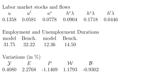
3.3.1 The Payroll Tax Exemption Reform
Table 6 highlights the results relative to the PTE reform. The policy increases the net production in the economy brought about by the large employment boost (as evidenced by the two point drop in unemployment). It succeeds in generating additional vacancies and job creation in the economy. The employment scale effect obtained here is consistent with other econometric studies on this topic (Kramarz and Philippon (2001); Cr´epon and Desplatz (2002); Laroque and Salani´e (2000) and (2002)). It must be noticed that the increase in the labor market tension leads to a decrease in the proportion of long-term unemployment. This feature contributes to improving the search efficiency in the economy. Human capital investment, however, contracts and capital stock decreases by 2.1233% and then the average productivity by 1.1469%. Note that this decrease in productivity is in the confidence interval of the estimation provided by Crepon and Desplatz (2002).
Contrary to the minimum wage case, the subsidy policy, as it is targeted at the low wages, may induce a negative productivity effect due to a distrib-ution effect which would then reinforce the investment channel. We evaluate the magnitude of these effects by comparing the variable productivity case with the constant investment one. The composition effect decreases the av-erage human capital E[k] and the avav-erage productivity P in the ki constant
case compared to the variable case (Table 7). This decline, due to the biased exemptions scheme, is particularly significant since higher rotations per se lead to a strong positive productivity effect (Table 5) when human capital investments are considered as given. The decline is further exacerbated if instead the investment varies, because of the decrease in human capital in-vestments following higher rotations in the economy. It is worth emphasizing that this last effect dominates the composition effect. It is only when aver-age productivity is maintained artificially unchanged that the PTE reform is
Table 6: The PTE Reform
Labor market stocks and flows
u ul us heλ hsλ hlλ
0.1358 0.0581 0.0778 0.0904 0.1718 0.0446
Employment and Unemployment Durations model Bench. model Bench.
31.75 32.22 12.36 14.50
Variations (in %)
Y E P W B
0.4080 2.2768 -1.1469 1.1793 -0.9302
Duration is expressed in months and stocks and flows in percentages
as efficient in increasing the net (only of hiring costs) production (1.4960% gain) as the optimal decrease of the minimum wage (1.4397% gain).
Table 7: Constant or Variable Productivity E× P − γv E E[k] P ki variable 0.3165 2.2768 -2.1233 -1.1469
ki constant 1.2125 2.2768 -1.3373 -0.2686
P constant 1.4960 2.2768 - -Variations in % relative to the benchmark calibration
While the PTE reform implies some direct budget cost, the welfare cri-terion can lead to a less optimistic evaluation22. Despite this budget cost,
the PTE reform implies an increase in welfare (∆W=1.1793%, Table 6) rela-tive to the benchmark economy, but also, and more unexpectedly, compared
22
The exemptions do not constitute the total budget variations: it is necessary to also take into account the reduction in unemployment benefits and the increase in payroll taxes collected from the employment boom.
to the optimal minimum wage level (∆W=1.0402%, Table 4). As long as the minimum wage is reduced to its optimal value, the employee value falls because of the decrease in the average wage. Introducing payroll tax exemp-tions, however, requires taking into account the decrease in dividends and in government lump-sum transfers. This decrease is spanned over all agents, yet the decrease in the minimum wage only concerns those employees at the bottom of the wage distribution. If the instrument is payroll taxes subsi-dies, the fall in employment costs for low-wage workers is supported by all agents. Alternatively, if the instrument is the minimum wage, the incidence applies only to low-wage workers. Given the concavity of the utility function, these changes in the distribution of total earnings are not neutral: the tax exemptions policy is considered superior to a decrease in the minimum wage.
3.3.2 Policy Choices: Targeting Subsidies around the Minimum Wage or Spreading over a Larger Range?
Do the PTE reforms lie on the optimal range of exempt wages? We take as given the shape of the policy and its direct cost. Our model is particularly well-suited for studying the consequences of this kind of policy. There is an explicit trade-off for a given budget cost: either the subsidies cover a narrow range and greatly reduce labor costs or they are spread over a larger range to avoid a downward distortion of the wage distribution.
The PTE reform is an intermediate scenario between a policy which con-centrates all exemptions at the minimum wage level and one which spreads payroll tax exemptions over the entire wage distribution. The first case mag-nifies the positive employment effect and the negative productivity impact. Table 8 shows that the balance is clearly against this policy. The second case tries to attenuate job allocation distortion, but at the expense of the magni-tude of the labor cost decline: only 2.65 points of payroll tax exemptions are possible to maintain the same budget cost as the PTE reform. Thus, this policy is overshadowed by the PTE reform, even if the human capital stock is higher (Table 8).
Table 8: Comparison with Two Extreme Cases
Y W E E(k) P
PTE Reform 0.4080 1.1793 2.2768 -2.1233 -1.1469 Uniform exemptions 0.1505 0.1965 0.4633 -0.4323 -0.2342 Exemptions at the mw -0.3738 0.1355 3.7240 -3.2394 -1.5667 Variations in % relative to the benchmark calibration
Given the same ex ante (direct) budget cost, the question remains whether we should further increase the subsidy at the minimum wage level or, on the contrary, spread out the subsidy over a wider range. However, the policy-maker faces uncertainty about the model parameters. We use the estimated covariance of the model parameters as a measure of this uncertainty. By mean of simulations23, ie. the random draw of parameter values from their
estimated law, we compute the confidence interval of the output and welfare changes shown in Figure 4. Let us note that the confidence interval is not very large which demonstrates the robustness of our policy results.
Figure 4: The Optimal Subsidy Scheme
1.2 1.4 1.6 1.8 2 0.2 0.25 0.3 0.35 0.4 0.45 threshold ∆ Output (%) 1.2 1.4 1.6 1.8 2 0.4 0.6 0.8 1 1.2 1.4 threshold ∆ Welfare (%)
It appears that the strategy of concentrating the subsidies more at the minimum wage level is output-reducing. More precisely, with regard to the production criterion, the optimal subsidy scheme increases continuously from 0% for jobs paid more than 1.36 times the minimum wage to 16% for jobs paid at the minimum wage (see Figure 4). With respect to the PTE reform, this particular shape optimally solves the trade-off between employment and pro-ductivity: net output increases by 0.4123%. Employment rises less (2.0961% in this case, 2.2768% in the case of the PTE reform), but capital falls at a lower rate (-1.9540% in this case, -2.1233% in the case of the PTE reform). Limiting the analysis to the employment side only would suggest using con-centrated exemptions around the minimum wage level. This paper shows that the conclusion dramatically changes when the productivity impact is considered. In this framework, spreading out exemptions over a wider distri-bution range appears more efficient.
By adding the welfare criterion, the analysis considers the concavity of the utility function and grants more importance to the decline in unemployment. Accordingly, the optimal scheme ranges up to 1.27 times the minimum wage, allowing more exemptions at the minimum wage level.
23
The simulation method is presented in Appendix E, as the distribution of the parame-ters used in the model simulations (Figure 5). The computation of this confidence interval takes 60 hours with a 2 MHZ Pentium 4 for 150 simulations and 23 policy schemes.