HAL Id: hal-01244298
https://hal.inria.fr/hal-01244298
Submitted on 15 Dec 2015
HAL is a multi-disciplinary open access
archive for the deposit and dissemination of
sci-entific research documents, whether they are
pub-lished or not. The documents may come from
teaching and research institutions in France or
abroad, or from public or private research centers.
L’archive ouverte pluridisciplinaire HAL, est
destinée au dépôt et à la diffusion de documents
scientifiques de niveau recherche, publiés ou non,
émanant des établissements d’enseignement et de
recherche français ou étrangers, des laboratoires
publics ou privés.
Implementation and measurements of an efficient Fixed
Point Adjoint
Ala Taftaf, Laurent Hascoët, Valérie Pascual
To cite this version:
Ala Taftaf, Laurent Hascoët, Valérie Pascual. Implementation and measurements of an efficient
Fixed Point Adjoint. EUROGEN 2015, ECCOMAS, Sep 2015, GLASGOW, United Kingdom.
�hal-01244298�
efficient Fixed Point Adjoint
A.Taftaf*, L. Hasco¨et and V.PascualAbstract Efficient Algorithmic Differentiation of Fixed-Point loops requires a spe-cific strategy to avoid explosion of memory requirements. Among the strategies documented in literature, we have selected the one introduced by B. Christianson. This method features original mechanisms such as repeated access to the trajectory stack or duplicated differentiation of the loop body with respect to different indepen-dent variables. We describe in this paper how the method must be further specified to take into account the particularities of real codes, and how data flow information can be used to automate detection of relevant sets of variables. We describe the way we implement this method inside an AD tool. Experiments on a medium-size appli-cation demonstrate a minor, but non negligible improvement of the accuracy of the result, and more importantly a major reduction of the memory needed to store the trajectories.
1 Introduction
The adjoint mode of Algorithmic Differentiation (AD)[3] is widely used in science and engineering. Assuming that the simulation has a scalar output, the adjoint algo-rithm can return its gradient at a cost independent of the number of inputs. The key is that adjoints propagate partial gradients backward from the result of the simulation. The main difficulty of Adjoint AD lies in the management of intermediate values. The computation of the partial gradients involves the partial derivatives of each run-time elementary computation of the original simulation. As these partial derivatives are needed in reverse execution order, and they use values from the original (forward order) computation, strategies must be designed to store or recompute these values. This has a cost that may be quite high, in extra computation time, storage memory
INRIA, 2004 Route des Lucioles, Sophia-Antipolis, France e-mail: {Elaa.Teftef, Laurent.Hascoet, Valerie.Pascual}@inria.fr
space, or both. Adjoint AD tools provide a number of such strategies, based on some combination of:
1. storage of intermediate values as the original simulation runs
2. re-computation of selected phases of the original simulation to retrieve these val-ues
3. inversion of some simple operations of the original algorithm
The specific AD tool that we develop basically relies on the first strategy (1). There-fore the structure of an adjoint code consists of a forward (FWD) sweep that runs the original code and stores the needed values, followed by a backward (BWD) sweep that retrieves the stored values and computes the derivatives. The above strategies are general, and as such are unable to take advantage of algorithmic knowledge of the specific simulation. On the other hand, exploiting knowledge of the algorithm and the structure of the given simulation code can yield a huge per-formance improvement in the Adjoint AD code. For instance, special strategies are available for parallel loops, long unsteady iterative loops, linear solvers... We fo-cus on the particular case of Fixed-Point (FP) loops, i.e. loops that iteratively refine a value until it becomes stationary. We call state the variable that progressively evolves as the FP loop runs till it reaches a stationary value and parameters the variables used by the FP iteration that influence the result but are never modified during the FP loop.
As FP algorithms start from some initial guess for the state, one intuition is that at least the first iterations are almost meaningless. Therefore, storing them for the adjoint computation is a serious waste of memory. Furthermore, FP loops that start with an initial guess almost equal to the final result converge only in a few iter-ations. As the adjoint loop of the standard AD adjoint code runs for exactly the same number of iterations, it may return a gradient that is not converged enough. For these reasons we looked for a specific adjoint strategy for FP loops. Among the strategies documented in literature, we have selected [7] the one introduced by B. Christianson [1, 2], in which the adjoint FP loop is a standalone new FP loop, that uses intermediate values from the last iteration only.
A FP equation
z∗= φ (z∗, x) (1)
where x is some fixed (set of) parameters, defines the converged state z∗as a function
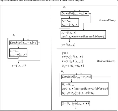
z∗(x) of x. Figure 1 (left) shows a code that solves iteratively the FP equation, until
reaching some stationarity of z by comparing zkwith zk+1and computes at the end
some final result y = f (z∗, x) by using the converged value of z.
B.Christianson’s special strategy [1] shown in figure 1 (right) keeps the standard structure of adjoint codes for everything before and after the FP loop. On the FWD sweep, the special strategy basically copies the original loop and inserts after it the FWD sweep of the FP loop body, in which it stores the converged value z∗and the
converged intermediate values occurring in the last FP iteration of z∗= φ (z∗, x). On
the BWD sweep, the method introduces a new FP loop with its own state variable wof the same shape as z and its own stopping criterion on stationarity of this new state. This adjoint loop solves the adjoint FP equation
y=1 z= y .∂ ∂zf ( z∗, x) x= y .∂ ∂xf (z∗, x) w0=z ; w1=w0+1 z∗=φ(z∗, x)
push( z∗+intermediate variables∈φ)
wk=wk +1
pop(z∗+intermediate variables∈φ)
wk+1=wk.∂∂zφ(z∗, x)+w0 x=w∗.∂∂xφ(z∗, x)+x w∗ Forward Sweep Backward Sweep zk=zk+1 zk+1=φ(zk, x) Do while (|zk +1−zk|>ϵ) y=f (z∗, x) zk=zk+1 zk+1=φ(zk, x) Do while(|zk +1−zk|>ϵ) z∗ z∗ y=f (z∗, x) Do while(|wk +1−wk|>ϵ)
Fig. 1 left: Example of code containing a FP loop with simple while loop, right: The special FP adjoint method applied at the FP loop
w∗= w∗.∂
∂ zφ (z∗, x) + z , (2)
which defines w∗ as a function of z (returned by the adjoint of the downstream
computation f ) through the adjoint derivative of φ with respect to z. The strategy terminates by computing the required x, using w∗and the adjoint derivatives of φ
with respect to x. Therefore, the method involves two different derivatives of φ . The above adjoint derivative computations repeatedly use the intermediate values stored by the last forward iteration, which are z∗ plus whatever was used to compute it
during the last iteration. As the specific adjoint method requires a repeated access to the stack, an extension of the standard stack mechanism has been defined in a previous work [7].
This paper focuses on the practical implementation of this special adjoint strat-egy. We describe how this strategy needs to be further specified in order to take into account the complexity of real codes. We describe how the various variables (state and parameters) needed by the adjoint can be automatically detected thanks to the data flow analysis of an AD tool. We describe the way we implement this strategy
in our tool Tapenade [5]. Finally, we validate our implementation on a medium-size code.
2 Acceptable shapes of Fixed-Point loops
Theoretical works about the FP loops often present these loops schematically as a while loop around a single call to a function φ that implements the FP iteration (see figure 1 (left)). FP loops in real codes almost never follow this structure. Even when obeying a classical while loop structure, the candidate FP loop may exhibit multiple loop exits and its body may contain more than only φ e.g. I/O. In many cases, these structures prevent application of the theoretical adjoint FP method.
For instance, a candidate FP loop might contain two exits as in figure 2 (left). Also the last iteration might not contain any computation of φ as in figure 2 (right). All these loops basically compute the same state variables and give exactly the same results as the one of figure 1, but the special adjoint strategy cannot be applied to them. This is due to the fact that the special adjoint method adjoins repeatedly the last iteration and thus this last iteration must contain the full computation of φ .
For these reasons, we need to define a set of sufficient conditions on the candidate FP loop. Obviously, the first condition is that the state variables reach a fixed-point i.e. their values are stationary during the last iteration, up to a certain tolerance ε. Moreover, the last iteration must contain the complete computation of φ . This for-bids loops with alternate exits, since the last iteration does not sweep through the complete body. Classically, one might transform the loop body to remove alternate exits, by introducing boolean variables and tests that would affect only the last iter-ation (see figure 2). We must forbid these transformed loops as well. To this end, we add the condition that even the control flow of the loop body must become stationary at convergence of the FP loop. This is a strong assumption that cannot be checked statically, but could be checked dynamically.
Conversely, the candidate FP loop could contain more than just φ . We must forbid that it computes other differentiable variables that do not become stationary. To enforce this, we require that every variable overwritten by the FP loop body is a part of the state, and therefore (from the first condition) is stationary. One tolerable exception is about the computation of the FP residual, which is not strictly speaking a part of φ . Similarly, we may tolerate loop bodies that contain I/O or other non-differentiable operations.
It may happen that the (unique) loop exit is not located at the loop header itself but somewhere else in the body. These loops can be transformed by unrolling, so that the exit is placed at the loop head, and the conditions above are satisfied. This unrolling is outside the scope of this work and we will simply require that the loop exit is at loop header.
We believe that these are sufficient applicability conditions of the strategy. Re-finements are possible, for instance, when two exits may be merged into one when
dz=|zk+1−zk| if (dz>ϵ) Do while (dz>ϵ) y=f (z∗, x) z∗ zk=zk+1 zk+1=φ(zk, x) dz=|zk+1−zk| if (dz>ϵ) Do while (convergence=false) y=f (z∗, x) z∗ zk=zk+1 zk+1=φ(zk, x) convergence=true
Fig. 2 left: Example of code containing a FP loop with two exits, right: Removing the alternate exit by introducing a boolean variable
no differentiable computation occurs between them. Such extensions of the method could be studied in further work.
3 Automatic detection of parameters and state
It is very hard or even impossible to detect automatically all FP loops in a given code. Statically, the AD tool cannot determine if every overwritten variable inside a loop will reach a fixed point. Therefore, we rely on the end-user to provide this information, for instance through a directive. As we required (in section 2) that the candidate FP loop has the syntactic structure of a loop, one directive, placed on the loop header, is enough to designate it. Thanks to AD-specific data-flow analysis, the AD tool can distinguish between the code that contains the computation of the state and the code that contains other non-differentiable operations, such as residual computation.
The program variables that form the state and the parameters can also be detected automatically from static data-flow analysis. Given the use set of the variables read by the FP loop, the out set of the variables written by the FP loop and the live set of the variables that are used in the sequel of FP loop, we can define:
state = out(FP loop) ∩ live (3)
parameters = use(FP loop)\out(FP loop) (4)
As we are only looking for differentiable influences of the parameters on the state, we may further restrict the above sets to the variables of differentiable type i.e. REAL or COMPLEX. In some cases, it may be instructive to let the user provide a larger set of state variables, probably adding extra variables that also reach a
sta-tionary value but are not needed in the sequel code. This is more a matter of style as the final gradient will not change. When on the other hand the data-flow analysis does not agree with the end-user choice, a warning message can be issued.
From a more technical standpoint, our specification of the state and parameters imposes a restriction on the use of arrays. In fact, our tool doesn’t distinguish in-dividual array elements during data-flow analysis. Arrays are considered as atoms. If an array is partly used to hold the state and partly to hold the parameters, our analysis cannot differentiate between the two parts. We therefore recommend that state variables and parameters are clearly identifiable so that the data-flow analysis can recognise them.
4 Specification of Implementation
4.1 Renaming the intermediate variables
The special FP adjoint, sketched in figure 1 (right), makes use of an intermediate ad-joint set of variables w which are temporary utility variables that do not correspond exactly to the adjoint of original variables. However, this w has the same size and shape as the state z.
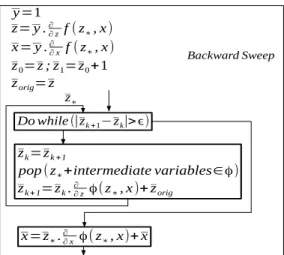
For implementation reasons, actual differentiation of the loop body is performed by a recursive call to the standard differentiation mechanism, which systematically names the adjoint variables after their original variables, so that w will actually be named z. The adjoint loop body must therefore have the form: zk+1= zk.φ (z∗, x). To
accommodate this form, we transformed the BWD sweep of the FP adjoint, intro-ducing in zoriga copy of the z, yielding the equivalent formulation shown in figure
3.
4.2 Specifying the transformation on Control Flow Graphs
As far as a theoretical description is concerned, it is perfectly acceptable to represent a FP loop with a simple body consisting of a call to φ . However, for real codes this assumption is too strong. We need to specify the adjoint transformation, so it can be applied to any structure of FP loops, possibly nested, that respect the conditions of section 2. Since these structures of interest inside a Control Flow Graph are obvi-ously nested, the natural structure to capture them is a tree. Therefore, our strategy is to superimpose a tree of nested Flow Graph Levels (FGLs) on the Control Flow Graph of any subroutine.
A FGL is either a single Basic Block or a graph of deeper FGLs. This way, the adjoint of a FGL is defined as a new FGL that connects the adjoints of the child FGLs and a few Basic Blocks required by the transformation. Adjoining a Flow
y=1 z= y .∂ ∂zf ( z∗, x) x= y .∂ ∂x f ( z∗, x) z0=z ; z1=z0+1 zorig=z zk=zk +1
pop (z∗+intermediate variables∈φ)
zk +1=zk.∂∂zφ(z∗, x)+ zorig
x=z∗.∂∂x φ(z∗, x)+ x
z∗
Backward Sweep
Do while (|zk +1−zk|>ϵ)
Fig. 3 Backward sweep of the FP adjoint method after renaming the intermediate variables
Graph is thus a recursive transformation on the FGLs. Every enclosing FGL needs to know about its children FGLs, their entry point, which is a single flow arrow, and their exit points, which may be many, i.e. many arrows. We introduce a level in the tree of nested FGLs, containing a particular piece of code, to express that this piece has a specific, probably more efficient adjoint. For instance, we introduce such a level for parallel loops, time-stepping loops, plain loops, and now for FP loops.
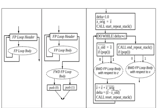
Specifically for a FP loop, the original FGL (see figure4 (left)) is composed of a loop header Basic Block and a single child FGL for the loop body. We arbitrarily place two cycling arrows after the loop body to represent the general case where one FGL may have several exit points. The FWD sweep of the FP loop adjoint (see figure 4 (middle)) basically copies the original loop structure, but inserts after this loop the FWD sweep of the adjoint of the loop body, thus storing intermediate values only for the last iteration. The BWD sweep (see figure 4 (right)) introduces several new Basic Blocks to hold:
• the calls that enable a repeated access to the stack.
• the computation of the variation of z into a variable delta which is used in the exit condition of the while loop.
• the initial storage of z into zorigand its use at the end of each iteration.
The FWD and BWD sweeps of the FP loop body, resulting recursively from the adjoint differentiation of the loop body FGL are new FGL’s represented in figure 4 by oval dashed boxes. They are connected to the new Basic Blocks as shown. The characteristic of the adjoint of a FP loop, visible in figure 3, is that the FP body must be differentiated twice, once with respect to z and once with respect to x. This accounts for the two FGL (oval dashed boxes) in figure 4, that stand for the two different adjoint BWD sweeps of the loop body.
BWD FP Loop Body with respect to z DOWHILE(delta>ϵ) delta=1.0 z_orig = z CALL start_repeat_stack() z_old = z
if (pop()) CALL end_repeat_stack()if (pop())
0 1
2
z = z + z_orig delta = (z - z_old) CALL reset_repeat_stack()
FP Loop Body FP Loop Body
FP Loop Header FWD FP Loop Body push (0) push (1) FP Loop Header 0 1 BWD FP Loop Body with respect to x 0 1
Fig. 4 left: flow graph level of a fixed-point loop, middle: flow graph level of the FWD sweep of this fixed-point loop, right: flow graph level of the BWD sweep of this fixed-point loop
4.3 Dead code elimination in recursive differentiation
In this implementation, the body of the FP loop is differentiated twice, by two re-cursive calls to the standard differentiation strategy on the loop body. Obviously this should bring some efficiency benefit since the two differentiations of the loop body are for different sets of independent variables (z and x). Therefore, some computa-tions may be active (i.e. are differentiated) in only one case and not the other, yield-ing shorter code. Other data-flow analysis performed automatically duryield-ing standard differentiation will bring additional benefit.
First, the code contained in the FP loop body and involved only in the compu-tation of the stopping criterion is detected as non-active, since it is used only in a test which is boolean, and therefore non differentiable. As a consequence, no ad-joint code will be generated for it in the two BWD sweeps. This applies also to non-differentiable code possibly present in the original FP loop. In other words, this guarantees that the adjoint code of the loop body computes only the derivative of the function φ , even if the original loop body may contain side computations.
Second, since there is no derivative code created in the BWD sweep(s) for com-putation of the stopping criterion and other non-differentiable code, the so-called dead-adjoint code analysis [4] finds that the primal intermediate values computed for evaluation of the stopping criterion are not used in the BWD sweep(s). They will therefore be eliminated from the FWD sweep which is added after the copy of
the original FP loop. Again, this makes the code shorter and clearer, as there is no reason to compute stopping criterion outside of any loop.
5 Experimental Results
For validation, we selected a real medium-size code which contains a FP loop. This code named GPDE is a Fortran90 program developed at Queen Mary University Of London (QMUL). It is a an unstructured pressure-based steady-state Navier-Stokes solver with finite volume spatial discretization. It is based on the SIMPLE (Semi-Implicit Method for Pressure Linked Equations)[6] algorithm for incompressible viscous flow computation.
The FP loop of the program computes the pression and velocity (the state vari-ables) of an incompressible flow by using the SIMPLE algorithm. In every iteration, the algorithm computes the velocity by solving the momentum equation. Then it uses the obtained value to compute the pression via solving the continuity equation. For comparison purposes, we differentiated GPDE with standard adjoint differenti-ation as well as with our special FP implementdifferenti-ation. We thus compare the standard FP adjoint with our special FP adjoint.
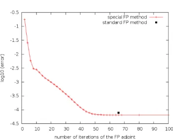
We observe a minor benefit on run-time and its link to accuracy. By construction, the standard FP adjoint runs for 66 iterations, which is the iteration count of the original FP loop. On the other hand, the special FP adjoint runs exactly as many times as needed to converge z. Figure 5 shows the error of the adjoint compared with a reference value (obtained by forcing the FP loop to run 151 times) as a function of the number of adjoint iterations for the special FP adjoint. For the standard FP adjoint, which runs exactly 66 iterations by construction, we have only one point on figure 5. For the special FP adjoint, we have a curve as the error decreases as iterations go. The special FP adjoint performs slightly better. For instance, it takes only 46 iterations to reach the same accuracy (7.8 ∗ 10−5) as the standard FP adjoint. This small improvement can be explained by the fact that the adjoint is computed using only the fully converged values.
The major benefit of the special method is about reduction of the memory con-sumption, since the intermediate values are stored only during the last forward iter-ation. The peak stack space used by the special adjoint is 60 times smaller than the space used by the standard adjoint (10.1 Mbytes vs. 605.5 Mbytes).
6 Further work
We have described an implementation of a specialized adjoint strategy for FP loops in an AD tool. Our first experiments produce efficient adjoint code, especially in terms of low memory consumption. There are a number of questions that might be studied further to achieve better results and wider applicability.
Fig. 5 Error mesurements of both standard and special fixed-point adjoint methods
The stopping criterion of the adjoint loop is reasonable, but so far arbitrary. The original article [1] gives indications of a better criterion. However, it is not clear to us whether we can implement it as is. In any case, the implementation might leave more freedom in the choice of this criterion.
Similarly, we have stated a number of restrictions on the structure of candidate FP loops. These are sufficient conditions, but we believe they can be partly lifted, for instance, when two loop exits can be considered as only one because the code between them is not differentiated. In other words, some restrictions on the shape of FP loops can be lifted at the cost of some loop transformation. The request that the flow of control becomes stationary at the end of the FP loop is essential, and we have no means of checking it statically in general on the source. However, it might be interesting to check it dynamically at run time.
In many applications, the FP loop is enclosed in another loop and the code takes advantage of this to use the result of the previous FP loop as a clever initial guess for the next FP loop. We believe that the adjoint FP loop can use a similar mech-anism, even if the variable w is not clearly related to some variable of the original code. However, we made such experiments by reusing the previous w. We were dis-appointed to find out that the benefit is limited, only decreasing the number of inner adjoint iterations by one or two percents.
Finally, this adjoint FP loop strategy is for us a first illustration of the interest of differentiating a given piece of code (i.e. φ ) twice, with respect to different sets of independent variables. This is a change from our tool’s original choice, which is to maintain only one differentiated version of each piece of code and therefore to generalize activity contexts to the union of all possible run time activity contexts. Following in this direction, a recent development in our tool jointly with students
from QMUL, allows the user to request many specialized differentiated versions of any given subroutine. An article describing the results is in preparation.
Acknowledgements This research is supported by the project “About Flow”, funded by the Euro-pean Commission under FP7-PEOPLE-2012-ITN-317006. See “http://aboutflow.sems.qmul.ac.uk”.
References
1. Christianson, B.: Reverse accumulation and attractive fixed points. Optimization Methods and Software 3, 311–326 (1994).
2. Christianson, B.: Reverse accumulation and implicit functions. Optimization Methods and Software 9, 307–322 (1998).
3. Griewank, A., Walther, A.: Evaluating Derivatives: Principles and Techniques of Algorithmic Differentiation. Other Titles in Applied Mathematics, 105. SIAM, (2008).
4. Hasco¨et, L., Araya-Polo, M.: The Adjoint Data-Flow Analyses: Formalization, Properties, and Applications. Automatic Differentiation: Applications, Theory, and Tools. Lecture Notes in Computational Science and Engineering, pp. 135-146. Springer (2005).
5. Hasco¨et, L., Pascual, V.: The Tapenade Automatic Differentiation tool: Principles, Model, and Specification. ACM Transactions On Mathematical Software 39(3) (2013)
6. Reuther, J., Alonso, J.J., Rimlinger, M.J., Jameson, A.: Aerodynamic shape optimization of supersonic aircraft configurations via an adjoint formulation on distributed memory parallel computers. Computers and Fluids 28(675700) (1999).
7. Taftaf, A., Pascual, V., Hasco¨et, L.: Adjoint of Fixed-Point iterations. 11th World Congress on Computational Mechanics (WCCM XI) 5, 5024–5034 (2014).