HAL Id: hal-01706142
https://hal.inria.fr/hal-01706142
Submitted on 10 Feb 2018
HAL is a multi-disciplinary open access
archive for the deposit and dissemination of
sci-entific research documents, whether they are
pub-lished or not. The documents may come from
teaching and research institutions in France or
abroad, or from public or private research centers.
L’archive ouverte pluridisciplinaire HAL, est
destinée au dépôt et à la diffusion de documents
scientifiques de niveau recherche, publiés ou non,
émanant des établissements d’enseignement et de
recherche français ou étrangers, des laboratoires
publics ou privés.
Lower Bounds for the Fair Resource Allocation Problem
Zaid Allybokus, Konstantin Avrachenkov, Jérémie Leguay, Lorenzo Maggi
To cite this version:
Zaid Allybokus, Konstantin Avrachenkov, Jérémie Leguay, Lorenzo Maggi. Lower Bounds for the Fair
Resource Allocation Problem. IFIP Performance 2017 - 35th International Symposium on Computer
Performance, Modeling, Measurements and Evaluation, Nov 2017, New York, United States. pp.1-7.
�hal-01706142�
Lower Bounds for the Fair Resource Allocation Problem
Zaid Allybokus
∗†, Konstantin Avrachenkov
∗, Jérémie Leguay
†and Lorenzo Maggi
† ∗INRIA Sophia Antipolis†Huawei Technologies, France Research Center
{zaid.allybokus, jeremie.leguay, lorenzo.maggi }@huawei.com
[email protected]
ABSTRACT
The α-fair resource allocation problem has received remark-able attention and has been studied in numerous application fields. Several algorithms have been proposed in the context of α-fair resource sharing to distributively compute its value. However, little work has been done on its structural proper-ties. In this work, we present a lower bound for the optimal solution of the weighted α-fair resource allocation problem and compare it with existing propositions in the literature. Our derivations rely on a localization property verified by optimization problems with separable objective that permit one to better exploit their local structures. We give a local version of the well-known midpoint domination axiom used to axiomatically build the Nash Bargaining Solution (or pro-portionally fair resource allocation problem). Moreover, we show how our lower bound can improve the performances of a distributed algorithm based on the Alternating Direc-tions Method of Multipliers (ADMM). The evaluation of the algorithm shows that our lower bound can considerably re-duce its convergence time up to two orders of magnitude compared to when the bound is not used at all or is simply looser.
Keywords
Weighted α-fairness; Resource allocation; Network utility maximization; Proportional fairness; Max-min fairness; Al-ternating Directions Method of Multipliers.
1.
INTRODUCTION
The α-fair resource sharing model, first studied in [Mo and Walrand], has already been investigated in numerous application domains, as well as its weighted variants. The weighted (w, α)-fair resource allocation problem is to find a vector x∗∈Rn+ such that 1) the utility
fα(w, x) = { ∑ni=1wi x1−αi
1−α, α ≠ 1,
∑ni=1wilog(xi), α = 1
is maximized at x = x∗, and 2) x∗ lies in a feasible set de-fined by linear constraints of the form Ax ⩽ c where c ∈ Rp+ is a capacity vector for a number p of resources and A is the binary user-resource incidence (p, n)-constraint matrix, for a number n of users, weighted by a positive vector w ∈ Rn+. The family of (w, α)-fair metrics is general and includes
IFIP WG 7.3 Performance 2017.Nov. 14-16, 2017, New York, NY USA Copyright is held by author/owner(s).
popular fairness concepts such as max-throughput (α = 0), proportional fairness, also called Nash Bargaining Solution (α = 1), min-delay (α = 2) and arbitrarily close approxima-tions of max-min fairness (α → ∞).
In this paper, we study the general weighted (w, α)-fair resource allocation problem under linear constraints and we propose a novel lower bound on its optimal solution. A lower bound is a positive vector d ∈ Rn+respecting feasibility (that is, Ad ⩽ c) and such that x∗ ⩾d. Finding a lower bound in the context of fair resource sharing is of great interest – it permits one to automatically define a minimal share that is attributable to each resource user as initialization of any exact computation that could take time, and may be helpful in the phase of design of a system. We seek to derive user-centric formulas in the sense that their value for a specific user would depend only on the resources within a localized problem (and not on the global topology) and only on the users that compete over the same resources. We then evaluate the formulas under different instance regimes and compare them to the literature in order to appreciate the improvements they provide.
Remarkably, we also show how our lower bound can en-hance the performance of a distributed algorithm based on the Alternating Directions Method of Multipliers (ADMM) (see [Boyd et al.]) that can be invoked to solve optimally the α-fair resource allocation problem. The ADMM is well-known for its fast convergence properties to modest accu-racy; however, its performance is highly conditioned by the initialization of its so-called penalty parameter that can, when badly tuned, induce an extremely poor convergence rate. Thus, tuning correctly the penalty parameter is a task that one should not neglect when using the ADMM. In light of recent studies (in particular, we exploit the results proven in [Deng and Yin]), we demonstrate how our lower bound permits one to accomplish this task for our particular prob-lem.
A well known lower bound of the proportionally fair (α = 1) resource allocation was brought in as a building block of the axiomatization of the Nash Bargaining Solution and is commonly referred to as the midpoint domination axiom [de Clippel]. It states that each user i is given at least a fraction wi
∑n
j=1wj of their dictatorial allocation, that is, the re-source they would receive if the other users accept to receive 0. We refer to the bound given by the midpoint domination axiom as the midpoint allocation. One can imagine that the midpoint allocation becomes arbitrarily poor as the total number of users becomes large, and its utility as a first es-timation of the optimum allocation, negligible. Indeed, the
formula includes the weights of the whole set of users and is independent of the problem’s local structure. Similarly, the general lower bound found in [Marasevic et al.] may suffer from these dependencies.
Concerning proportional fairness (α = 1), we give a more precise midpoint domination axiom, and provide a lower bound that we call local midpoint. Our lower bound on the proportionally fair allocation can be interpreted as a particular case of the midpoint domination axiom to local-ity – now, each user i is proportionally fairly attributable at least a fraction wi
∑j∈Siwj of their dictatorial allocation, where Si is not the total set of users, but the set of users
in competition with the user i for some resource. Few works attempted at providing lower bounds for the general (w, α)-fair resource allocation. In fact, the most recent available bound is shown by [Marasevic et al.], and used by the au-thors for an initialization of their α-fair heuristic. To the best of our knowledge, this is the best bound that could be found in the literature for the α-fair resource allocation problem and we refer to it as the State-of-the-Art (SoA).
The remainder of the paper is organized as follows: Sec-tion 2 is dedicated to the model definiSec-tion and problem statement. Our lower bound presentation is addressed in Section 3. In Section 4, we broadly remind the key features of the ADMM-based α-fair distributed algorithm used for our illustration. The performance of the latter is shown in Section 5 and finally, Section 6 concludes the paper.
2.
MODEL DEFINITION
Let us start by formalizing the weighted α-fair resource allocation problem. In this work, we adopt the terminology of rate control in fixed communication networks. Thus, a resource will be referred to as a link and a user will be called a connection request (or shortly, request ) from a source node to a destination node over a route formed of several links.
Let J be the set of network links, each link j having a capacity cj∈R+. Let R be the set of requests. Each request r has a predefined route that identifies with a subset Jr ⊂ J of links of the network. In turn, for each link j ∈ J , Rj∶= {r ∈ R; j ∈ Jr}is the set of all requests having a route that contains the link j. We define the link-route incidence ∣J ∣ × ∣R∣-matrix A as:
Ajr= { 1 if j ∈ Jr 0 otherwise
For each request r, xr denotes the bandwidth allocated to
r along its route Jr. We say that an allocation x = (xr)r∈R belongs to the feasibility set C (or is feasible) if it satisfies the capacity constraint (1) below:
x ∈ C ⇔ Ax ⩽ c, x ⩾ 0 (1) where c = (cj)j∈J. Each request r is associated with a weight wr ∈R+. The weight vector w = (wr)r∈R accounts for a degree of relative importance of each request that can be defined at the discretion of the network. Weighted α-fairness is formalized as in Definition 1 below.
Definition 1 ((w, α)-fairness). Let C ⊂ R∣R∣+ be a feasibility set defined as in (1), being a strict superset of {0}. Let w ∈ R∣R∣+ and x∗∈C. We say that x∗is (w, α)-fair (or simply α-fair when there is no confusion on w) if the
following holds: ∀r ∈ R, x∗r>0 and ∀x ∈ C, ∑ r∈R wr xr−x∗r x∗αr ⩽0. Equivalently, x∗is (w, α)-fair if, and only if x∗ maximizes the α-fair utility function fα defined over C − {0}:
max x∈C f α (w, x) = ∑ r∈R frα(wr, xr), (Pα) where frα(wr, xr) = { wr x1−αr 1−α, α ≠ 1, wrlog(xr), α = 1.
3.
ALPHA-FAIRNESS – A LOWER BOUND
In this section, we derive an explicit lower bound on the general (w, α)-fair resource allocation problem. Our lower bound only depends on the weight vector w, the capacity vector c and the link-route incidence matrix A. Moreover, the bound exploits the local structure of the problem, which prevents it from deteriorating systematically with the prob-lem size. We compare it to the SoA bound that one can formulate as follows:
Proposition 1 ([Marasevic et al.]). Let the vector x∗ be the optimal solution to the α-fair resource allocation problem. Then, for all r ∈ R:
● if 0 < α ⩽ 1, x∗r⩾mr(α) ∶= (wmaxwrMmin j∈Jr cj ∣Rj∣ ) 1/α c1−1/αmax ● if α > 1, x∗r⩾mr(α) ∶= ( wr wmaxM) 1/α min j∈Jr cj ∣Rj∣ (cmin cmax ) 1−1/α
where wmax=max wr, M = min{∣R∣, ∣J ∣}, cmin=min cj and
cmax=max cj.
We seek to improve the above bound by removing the global dependencies on wmax, ∣Rj∣, and M , cmin and cmax,
those parameters being the major degradation factor when the size or congestion of the problems increase.
For each request r ∈ R, let br∶=minj∈Jrcj. The so-called utopia point b ∶= (br)r∈Ris the (infeasible when the problem is non trivial) allocation representing the value each request would receive if they were alone in the network, that is, its dictatorial allocation. Our bound for the (w, α)-fair alloca-tion only depends on the utopia point (hence on the capacity vector c), the matrix A and on the weight vector w. For r ∈ R, let Rr∶= {s ∈ R; Jr∩Js≠ ∅}, i.e., the set of requests
sharing at least one resource with r andRr∶=R − Rr
. First of all, we use the separability of the objective func-tion of Problem (Pα) to better estimate our lower bound
on a restricted problem. Specifically, we prove a restriction lemma (see Lemma 1) that permits one to avoid unnecessary dependencies between requests that do not share resources together. Then, we prove our general lower bound on the corresponding restricted problems. Thanks to Lemma 1, the bound remains unchanged in the original problem.
3.1
A restriction lemma
In this paragraph, we show that instead of evaluating our bound on Problem (Pα), one can use a smaller
request-centric problem. Specifically, let x∗denote the optimal solu-tion of Problem (Pα) and let r0∈R be an arbitrary request. We define the restricted problem at r0, as the following:
min ∑ r∈Rr0 −frα(wr, xr) ( ̃Pr0) s.t. ∑ r∈Rj∩Rr0 xr⩽˜cj∶=cj ∀j ∈ Jr0 and ∑ r∈Rj∩Rr0 xr⩽˜cj∶=cj− ∑ r∈Rj∩Rr0 x∗r ∀j ∈ J − Jr0.
Intuitively, Problem ( ̃Pr0) arises when the allocations of all the requests that do not share any link with r0are fixed to
their optimal α-fair value (that is, following the vector x∗), and one needs to compute the α-fair allocation of the re-maining requests, that is, the requests within Rr0that share at least one resource with r0. The capacity constraints are
thus updated taking into account the amounts of resources that are already allocated, as shows the second line of the constraints. Note in passing that all the links in J − Jr0 that do not serve any of the requests within Rr0 form trivial constraints in ( ̃Pr0) and can hence be removed without any loss.
We then have the following result:
Lemma 1. The restriction to (P̃r0) does not change the optimal allocation of the remaining requests: if x is the opti-mal solution of the Problem ( ̃Pr0), then, xs=x
∗
s, for s ∈ R r0. Proof. Consider the problem:
min ∑
r∈R
−frα(wr, xr) (2)
s.t. Ax ⩽ c xr⩾x∗r ∀r ∈ Rr0.
It suffices to show that the problems (2) and ( ̃Pr0) are equiv-alent. Then, the unicity of the solutions permits one to con-clude.
We know that the problem (2) is feasible, as x∗is a fea-sible point. Denote its optimal solution by ˜x. We remark that both x∗and ˜x are feasible for both problems (Pα)and (2). Hence, by optimality, we necessarily have fα(w, ˜x) = fα(w, x∗). Moreover, for instance, problem (P
α) has a unique optimal solution. Thus,
x∗=x.˜
Particularly for r ∈Rr0, x∗r=x˜r. Thus, we can fix the values
xr=x∗r for r ∈ Rr0 without changing the optimum. Thus, Problem (2) is equivalent to the restricted problem ( ̃Pr0).
Thanks to Lemma 1, we are now ready to present our lower bound on the α-fair allocation based on the structure of the restricted problems.
3.2
Lower bound
We now show the main result of this paper. We define the local midpoint p as the following:
∀r ∈ R pr∶= wr ∑
s∈Rr ws
br.
Theorem 1. Let x∗ denote the optimal solution of prob-lem (Pα). Let r0 ∶=argmins∈Rps. Then, x∗ can be lower
bounded as follows: ● if α ⩾ 1, ∀r ∈ R x∗r⩾dr(α) ∶= p1−1/αr0 p 1/α r ● if 0 < α ⩽ 1, ∀r ∈ R x∗r⩾dr(α) ∶= ⎛ ⎜ ⎜ ⎝ wrbr ∑ s∈Rr wsb1−αs ⎞ ⎟ ⎟ ⎠ 1/α .
Proof. We first prove the proposition for α ⩾ 1. Let us define the request rminas the request with the least optimal
allocation: rmin=argmins∈Rx∗s. By definition of r0, we have:
prmin⩾pr0 (3) Let r ∈ Rr. By Lemma 1, it suffices to show the inequality in the restricted problem (̃Pr)associated to r. Let Cr denote its feasible set. Thus, for all (xs)s∈Rr∈Cr we have:
∑ s∈Rr ws xs−x∗s x∗αs ⩽0,
This inequality holds for all feasible (xs)s∈Rr ∈Cr. Thus, we evaluate it at the dictatorial allocation of r, that is, at the point x defined as xr= ˜brand xs=0 for all s ∈ Rr− {r}. Let us note in passing that ˜br=minj∈Jr˜cj=minj∈Jrcj=br.
Thus, wr˜br=wrbr⩽x∗αr ∑ s∈Rr wsx∗1−αs ⩽ ( ∑ s∈Rr ws)x∗1−αrminx ∗α r ,
where we remind that rmin = argmins∈Rx∗s and 1 − α ⩽ 0. Rearranging the terms, one gets:
wrbr ∑ s∈Rr ws x∗α−1rmin ⩽x ∗α r , which yields: p1/αr x∗1−1/αrmin ⩽x ∗ r (4)
In particular, applying equation (4) to r = rmin, we get:
x∗rmin⩾prmin⩾pr0 (5) Finally, we plug equation (5) in equation (4) to obtain the desired lower bound on x∗r (because 1 − 1/α ⩾ 0).
Next, we show the bound for 0 < α < 1. In the same fashion, we look at the restricted problem. Let r ∈ R and consider its restricted problem. Then, one has:
wrbr x∗αr ⩽ ∑ s∈Rr wsx∗1−αs ⩽ ∑ s∈Rr ws˜b1−αs ⩽ ∑ s∈Rr wsb1−αs .
Rearranging the terms finally provides the desired bound. For any value of α, one can remark that the bound (dr(α))r∈R only depends on the capacity vector c, the weight vector w, and the link-route incidence matrix A.
3.3
Illustration
To conclude this section, we illustrate a comparison of the two presented lower bounds m and d introduced in Proposi-tion 1 and Theorem 1, respectively, under different regimes. Given the formulas, one can remark that the sensitivity of the bound to arbitrary problem sizes should be lessened as now more focused on local structures. For α ⩽ 1, we obtain request-centric formulas. For general α > 1, this elimina-tion came with the dependency on the global minimum local
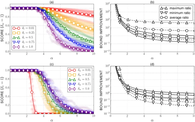
Figure 1: A comparison of the two bounds. The scores, and the minimum, average and maximum bound improvements are illustrated in the cases of (a)-(b) a constant δwfor different values of δc, and of (c)-(d) a constant δcfor different values of δw. Figures (b) and (d)
show the bound improvements in the two extreme situations δc(resp. δw) = 0.01 (resp. 1) in dashed lines (resp. solid lines).
midpoint value pr0. Intuitively, one can remark that the two bounds may react differently to a fluctuating asymmetry of the weight vector w or the capacity vector c, namely, a vari-ation of the two parameters δw∶=max wmin wr
r and δc∶=
cmin
cmax. For a better vision, we illustrated this behavior in Figure 1.
The two bounds were compared on instances with 1000 requests over a same graph of type barabasi(100,4) (see [Al-bert and Barabási]). The routes were generated at random by taking the shortest path between pairs of sources and destinations drawn uniformly at random. The weights (resp. link capacities) were also drawn uniformly at random within intervals I satisfying inf I/ sup I = δw (resp. δc). For each
instance, and each α, we define the score of d as the number ∣{r ∶ dr(α) > mr(α)}∣/∣R∣. The score represents the
propor-tion of requests for which our bound d(α) beats the SoA bound m(α) for a particular α. In Figure 1(a), the param-eter δw was fixed to 1 (which namely means w = 1) and
we plotted the score of d versus α for different values of δc.
Figure 1(c) shows the score in the other extreme situation δc = 1 (which means all the link capacities are equal) for different values of δw.
In order to appreciate the quality of the bound improve-ment, if any, we plotted, in Figures 1(b) and 1(d), the corre-sponding bound improvements, measured with the values of the ratios dr(α)/mr(α). To preserve readability of the plots,
we represented only the extreme situations corresponding to the values δc =0.01 (dashed lines) and δc =1 (solid lines)
for Figure 1(b) and to the values δw =0.01 (dashed lines) and δw =1 (solid lines) for Figure 1(d). Figures 1(b) and 1(d) show the best, worst, and average improvements en-countered in the same problem instance. All the points represented in Figure 1 correspond to an average over 10 in-stances generated under identical conditions. In Figures 1(a) and 1(c), we also included the specific points as translucent scattered markers.
According to Figure 1, our bound is an absolute improve-ment for values of α in the interval [0,2] (thus including the max-throughput, proportional fairness, and min-delay pop-ular concepts) in all situations. Particpop-ularly for proportional fairness, the simulations show that we improved the bound m by two orders of magnitude in all situations. For min-delay fairness, the bound is generally improved on average by a multiplicative factor between 1 and several tens. For greater values of α, it is interesting to see that either d or m is more adapted to certain problem structures. For in-stance, d will be of greater interest when the network link capacities are more heterogeneous, δc≪1 (which may cor-respond to situations where the network is asymmetrically congested), whereas m is more adapted to asymmetrically weighted problems, δw ≪ 1. One can thus conclude that the two available bounds complement each other for general α ⩾ 1.
After presenting our bound, we now demonstrate how it permits one to boost the performance of an algorithm that
solves the (w, α)-fair resource allocation problem.
The next section is dedicated to the presentation of the algorithm, based on ADMM.
4.
FAST AND DISTRIBUTED ADMM
(FD-ADMM)
Several approaches may be used to tackle the (w, α)-fair resource allocation problem (e.g., see [Kelly et al.] and [Palo-mar and Chiang] for a tutorial). One of them is the Alter-nating Directions Method of Multipliers (ADMM) (see, e.g., [Boyd et al.]). The ADMM is well known for its distributiv-ity properties that permit one to decouple constraints han-dled in parallel then plugged in together by means of con-sensus constraints. In [Allybokus et al.], these properties are used to design a fully distributed algorithm that solves optimally the problem in the context of traffic rate control in distributed Software-Defined Networks. For a description of the general ADMM framework, the reader may refer to [Boyd et al.], and for a more detailed construction of the presented algorithm, to [Allybokus et al.]. In this section, we briefly describe the design of the distributed algorithm used in the latter.
4.1
Algorithm overview
Assume the network links are split into a number P ⩾ 1 of domains. Each domain p corresponds to a subset Jp⊂J of links forming a covering of the whole set J :
P
⋃
p=1Jp
=J.
For p = 1 . . . P , let Rp = {r ∈ R, Jp∩Jr ≠ ∅} be the set of requests that traverse domain p, and Ir= {q ∈ [1, P ]; r ∈ Rp} the set of domains the request r traverses. The problem (Pα)
can thus be rewritten as: : min x∈Cr∈R∑−f α r(wr, xr) =min x∈C P ∑ p=1r∈R∑p − 1 ∣Ir∣ frα(wr, xr) =min x P ∑ p=1 ⎧ ⎪ ⎪ ⎨ ⎪ ⎪ ⎩ ιp(x) + ∑ r∈Rp − 1 ∣Ir∣ frα(wr, xr) ⎫ ⎪ ⎪ ⎬ ⎪ ⎪ ⎭ ∶=min x P ∑ p=1 ιp(x) + gp(w, x), (6)
where ιp is the indicator function of the capacity subset
associated to domain p: ιp(x) = ∑ j∈Jp ιj(x), ιj(x) = ⎧ ⎪ ⎪ ⎨ ⎪ ⎪ ⎩ 0 if ∑ r∈Rj xr⩽cj ∞ otherwise Further, we separate artificially the problem by creating a private variable xp∈R∣Rp∣for each domain p, and by enforc-ing the agreement upon their values between domains with consensus constraints. Problem formulation (6) now reads:
min P ∑ p=1gp (w, xp) +ιp(xp) s.t xpr=xqr ∀p, q ∈ Ir ∀r ∈ R (7) xp∈R∣Rp∣ ∀p = 1 . . . P.
Algorithm 1 Fast Distributed ADMM (FD-ADMM) 1: procedure of Domain p
2: Receive ˜zp= (˜zr)r∈Rp
3: Receive updated reciprocal penalty λ0from master 4: for j ∈ Jpdo 5: ujr←ujr+yjr−z˜pr ∀r ∈ Rj 6: yj←P(j, ˜zp−uj) 7: end for 8: for r ∈ Rpdo 9: vpr←vpr+xpr−z˜pr 10: xpr←argminx{−frα(wr, x) +2λ1 0∣∣x − (˜zpr−vpr)∣∣ 2 } 11: end for 12: end procedure 13: procedure of Master
14: Compute lower bound d and λ0using Eq. (10) 15: while termination condition not met do
16: λ0←λ updated using RB, by [He et al.] 17: for r ∈ R do 18: 19: z˜r←∣J 1 r∣+∣Ir∣(∑j∈Jryjr+ ∑q∈Irxqr) 20: end for 21: for p ∈ P do 22: Send ˜zp= (˜zr)r∈Rp to domain p 23: end for 24: end while 25: end procedure
Finally, we decompose the problem by separating the pri-vate objective of each domain. For each domain p, and each j ∈ Jp, the vector yj defines a copy of the variable xp for
link j and is reserved for the component function ιj. We
can write Problem (7) in the following form:
min P ∑ p=1gp (w, xp) + ∑ j∈Jp ιj(yj) ∶= ∑ p∈PGp (w, xp, yp) s.t xpr=xqr ∀p, q ∈ Ir ∀r ∈ R (8) xpr=yjr ∀j ∈ Jp ∀r ∈ Rj xp∈R∣Rp∣ ∀p = 1 . . . P yj∈R∣Rj∣ ∀j ∈ J yp= (yj)j∈Jp ∀p ∈ P
Let χ denote the indicator function of the feasible set (8). Then, the formulation takes the compact 2-block form:
min ∑ p∈PGp (w, xp, yp) +χ((x′p)p∈P, (yp′)p∈P) (9) s.t. (xp, yp) = (x′p, y ′ p)
Applied to the last formulation (9), the distributed ADMM is described in Algorithm 1. In lines 5 and 10, the variables uj∈R∣Rj∣and vp∈R∣Rp∣ are dual variables associated with the constraints {yj=y′j}and {xp=x′p}, respectively in (9). Also, P(j, ⋅) is the Euclidean projection onto the simplex {yj∈RRj s.t. yjr⩾dr and ∑r∈Rjyjr⩽cj}, λ > 0 is a scalar reciprocal penalty parameter, and d ∈ RR is a lower bound on the (w, α)-fair solution that will be computed with the input parameters.
4.2
Performance
The convergence of ADMM is provably known since the 1990s (see [Eckstein and Bertsekas]), and its convergence rate has been widely studied. Today, the most general con-vergence rate of ADMM is known to be O(1/T ) (T being the iteration count), and linear convergence rates are prov-ably obtained for strongly convex problems. Nevertheless, the performance of the ADMM remains highly sensitive to the initialization and the update of the penalty parameter. In [Deng and Yin], the linear convergence rate of ADMM for strongly convex problems is quantified and optimized with regards to the penalty parameter, which yields an optimal tuning of it. Its value depends on the (global) strong convex-ity and the Lipschitz gradient moduli of the objective func-tion, if those are finite. In [Allybokus et al.], this result is applied to a central strongly convex equivalent formulation of our problem to derive an approximate adaptive tuning of the distributed version of the algorithm. The adaptive penalty parameter is computed as the optimal parameter of the centralized formulation, λ0, given according to the
formula
λ0= 1 √
σL, (10) where σ is the strong convexity modulus of fα(w, ⋅) and L is the Lipschitz modulus of its gradient. In fact, the fairness functions have singular values near 0, which make the Lip-schitz modulus not globally defined, unless the feasible set is reduced from below by means of a positive lower bound d of the optimal solution. Thus, Equation (10) is applied to L = Ld where Ld is the Lipschitz modulus of the gradient
of the objective over the set of feasible points x verifying x ⩾ d.
Adaptive penalty parameter schemes have been proposed to tackle this issue and provably bring consistent improve-ment of the convergence behavior of ADMM. One remark-able adaptive scheme can be found in [He et al.], in which the authors introduce the residual balancing (RB) principle which consists of shrinking or expanding the penalty param-eter whenever the primal and dual residuals are unbalanced. For a definition of RB, we refer the interested reader to [He et al.]. Although this scheme helps making the ADMM less dependent from initialization, empirical behaviors of the al-gorithm however suggest that there is still room and inter-est for better initialization. To demonstrate this, we adopt residual balancing as a default adaptive scheme of our penal-ties in all the algorithms of the present paper.
In Section 3, we introduced the lower bound d (Theo-rem 1) on the (w, α)-fair optimal allocation. Next, we demonstrate how this bound permits one to enhance the performance of the ADMM for the (w, α)-fair resource al-location problem, and we compare it with the performance brought by the SoA bound m (Proposition 1). Although the lower bound permits one to adjust quickly a minimal individual resource allocation that would never be violated during the running time of the algorithm, the major feature of its introduction is in that it permits one to define an ini-tialization of the penalty parameter that could enhance the algorithm performance. Indeed, the initialization can pro-vide spectacular convergence acceleration, whereas reduc-ing the feasible set at the projection line 6 of Algorithm 1 does not seem to matter, illustrating the fast convergence of FD-ADMM to modest accuracy. These observations are illustrated in the next section.
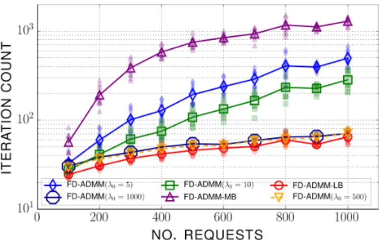
Figure 2: Iteration count versus the number of connection re-quests in situation 1. For FD-ADMM-LB and FD-ADMM-MB, the reciprocal penalty initialized value λ0lies in [110-150] and in
[1, 6], respectively.
5.
EXECUTION
In the present simulations, we dedicate our performance evaluation to the proportionally fair resource allocation prob-lems (α = 1). In this section, we demonstrate the gains achievable with only tuning the initial penalty parameter of the FD-ADMM by comparing several initialization schemes. Indeed, the only difference between the different algorithms that we compare is in that the initial penalty parameter λ0is
chosen either arbitrarily – FD-ADMM(λ0=λ), or according to Equation (10) applied to the bound m (FD-ADMM-MB) or d (FD-ADMM-LB).
The problem instances were generated under the same conditions as in Section 3.3. As it appears the parameter δw
can deteriorate importantly the quality of our bound when small, we execute the simulations under two different situa-tions 1) wr∈ [.9, 1], and 2) wr∈ [.1, 1].
Performance results
In Figures 2 and 3, we plotted the iteration count of the algorithms under situations 1 and 2, respectively. The al-gorithms stop when the primal and dual residuals of the ADMM algorithm (see, e.g., [Boyd et al.]) fall below 10−2 (relatively modest accuracy). For each problem size in terms of number of different requests, we generated 10 instances of the corresponding size randomly and plotted the aver-age performance. The specific points are also represented with scattered translucent markers to account for the exact performance of each algorithm. For each situation, we ob-served the performances of FD-ADMM-LB, in particular, its average initial reciprocal penalty parameter given by Equa-tion (10) and chose several initializaEqua-tion values below and above this average to account for the effect of this initializa-tion on the algorithm’s performance.
Situation 1 (Figure 2). We observe a spectacular im-provement of the FD-ADMM algorithm from the scheme FD-ADMM-MB to the scheme FD-ADMM-LB, correspond-ing to a reduction of the runncorrespond-ing iteration count of two or-ders of magnitude. When λ0 is chosen larger than the one
for FD-ADMM-LB, although the performances seem satis-factory, one can observe that FD-ADMM-LB still executes faster on average.
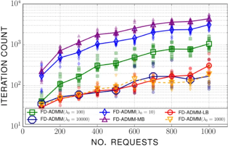
Figure 3: Iteration count versus the number of connection re-quests in situation 2. For FD-ADMM-LB and FD-ADMM-MB, the reciprocal penalty initialized value λ0 lies in [500,1000] and
in [0.1, 2.5], respectively.
Situation 2 (Figure 3). The same improvement of the performances, related to the introduction of our lower bound, is observed. It seems that for lower initialization value of λ0, the algorithms demonstrate poorer performances.
Nevertheless, one can observe that higher values of λ0 can
provide algorithms with, although not consistently, better performances than FD-ADMM-LB on average. Although this phenomenon can seem surprising after a look at situa-tion 1, one can explain it with the fact that when the vector w is highly unbalanced (as it is the case when its values are uniformly drawn at random within [.1, 1]) the objective function fα(w, ⋅) obtains highly asymmetric structure. In-deed, the computation of the strong convexity modulus of fα in [Allybokus et al.] in order to obtain a desirable ini-tialization λ0, shows that the factor σ in Equation (10) in
fact corresponds to the smaller strong convexity modulus of the functions frα(wr, ⋅), which is proportional to wr. Not
surprisingly then, this evaluation becomes poorer when the vector w becomes unbalanced. Thus, it is worth considering that an accurate penalty parameter tuning becomes more difficult when the weighted fairness function symmetry is poor. Nevertheless, our simulations suggest that initializing the reciprocal penalty parameter according to Equation (10) applied to our lower bound permits one to obtain a satisfac-tory performance of the FD-ADMM. We believe this scheme can be improved in order to tackle a potential performance issue under highly asymmetric realizations of the (w, α)-fair resource allocation problem characterized by a very low value of δw.
6.
CONCLUSION
We studied the structure of weighted (w, α)-fair alloca-tion problems and proposed a lower bound that permits one to better understand the problem’s features. The (w, α)-fair allocation can be lower bounded individually and locally (that is, each user, or request, has a minimal guarantied alcation that depends on its individual weight and that of a lo-cally reduced subset of users). We compared experimentally our bound with the best bound available in the literature, and showed that we can provide consistent improvement in the case of high asymmetry of the capacity vector c (which
may describe congested networks situations) or in the case of a suitable symmetry of the fairness measures (which may cover situations where the requests have balanced relative priorities). We believe that the bound derived in the present paper for general fairness concepts (α > 1) can be further im-proved, and intend to soften its dependencies on the global minimum local midpoint value pr0. Our intuition suggests this would improve considerably the quality of our general bound. To demonstrate the utility of our derivation, we showed as an illustration how the introduction of this lower bound can remarkably improve the performances of an iter-ative distributed algorithm, the FD-ADMM, that solves the problem optimally, by a simple initialization of a penalty parameter. We also observed that the initialization scheme allows a remarkably satisfactory tuning of the FD-ADMM, and that this accuracy may impoverish as the asymmetry of the weighted problem strengthens. In the future, we envision to study this situation and strengthen our bound in order to possibly empower the initialization scheme, providing more robustness to the technique with respect to asymmetry.
References
Réka Albert and Albert-László Barabási. 2002. Statistical me-chanics of complex networks. Rev. Mod. Phys. 74 (Jan 2002), 47–97. Issue 1.
Zaid Allybokus, Konstantin Avrachenkov, Jérémie Leguay, and Lorenzo Maggi. 2017. Real-Time Fair Resource Allocation in Distributed Software Defined Networks. In 29th International Teletraffic Congress (ITC). 19–27.
Stephen Boyd, Neal Parikh, Eric Chu, Borja Peleato, and Jonathan Eckstein. 2011. Distributed optimization and statisti-cal learning via the alternating direction method of multipliers. Foundations and Trends in Machine Learning 3, 1 (2011), 1– 122.
Geoffroy de Clippel. 2007. An axiomatization of the Nash bar-gaining solution. Social Choice and Welfare 29, 2 (01 Sep 2007), 201–210.
Wei Deng and Wotao Yin. 2016. On the global and linear con-vergence of the generalized alternating direction method of mul-tipliers. Journal of Scientific Computing 66, 3 (2016), 889–916. Jonathan Eckstein and Dimitri P. Bertsekas. 1992. On the Douglas—Rachford splitting method and the proximal point al-gorithm for maximal monotone operators. Mathematical Pro-gramming 55, 1 (01 Apr 1992), 293–318.
BS He, Hai Yang, and SL Wang. 2000. Alternating direc-tion method with self-adaptive penalty parameters for mono-tone variational inequalities. Journal of Optimization Theory and applications 106, 2 (2000), 337–356.
Frank P Kelly, Aman K Maulloo, and David KH Tan. 1998. Rate control for communication networks: shadow prices, pro-portional fairness and stability. Journal of the Operational Re-search society 49, 3 (1998), 237–252.
Jelena Marasevic, Clifford Stein, and Gil Zussman. 2016. A Fast Distributed Stateless Algorithm for alpha-Fair Packing Problems. In 43rd International Colloquium on Automata, Lan-guages, and Programming (ICALP 2016) (Leibniz International Proceedings in Informatics (LIPIcs)), Vol. 55. 54:1–54:15. Jeonghoon Mo and Jean Walrand. 2000. Fair end-to-end window-based congestion control. IEEE/ACM Transactions on Networking (ToN) 8, 5 (2000), 556–567.
Daniel Pérez Palomar and Mung Chiang. 2006. A tutorial on decomposition methods for network utility maximization. IEEE Journal on Selected Areas in Communications 24, 8 (2006), 1439–1451.