Version postprint
Tree Algorithms
J. Stéphane Bailly, Anne Biarnes, Philippe Lagacherie
UMR INRA-IRD-SupAgro LISAH, Campus de la Gaillarde, 2 place Viala, 34060 Montpellier (France)
e-mail: [email protected], [email protected], [email protected]
Abstract
In this paper, extensions of the classification tree algorithm and analysis for spatial data are proposed. These extensions focus on: (1) a robust man-ner to prune a classification tree to smooth sampling (e.g., spatial sampling effects), (2) an assessment of tree spatial prediction performances with re-spect to its ability to satisfactorily represent the actual spatial distribution of the variable of interest, and (3) a unified framework to aid in the inter-pretation of the classification tree results due to variable correlations. These methodological developments are studied on an agricultural prac-tices classification problem at an agricultural plot scale, specifically, the weed control practices on vine plots over a 75 km² catchment in the South of France. The results show that, with these methodological developments, we obtain an explicit view of the uncertainty associated with the classifica-tion process through the simulaclassifica-tion of the spatial distribuclassifica-tion of agricul-tural practices. Such an approach may further facilitate the assessment of model sensitivities to categorical variable map uncertainties when using these maps as input data in environmental impact assessment modelling. Keywords: CART, uncertainties, stochastic spatial simulation, robustness, predictors correlation
Version postprint
1. Introduction
Classification tree analysis (Breiman et al, 1984) is a very popular data mining tool that has been widely applied within the last 20 years in many different disciplines, including landscape ecology (McDonald and Urban, 2006, Fearer et al., 2007), soil science (Lagacherie and Holmes, 1997, Bui and Moran, 2001), agronomy (Tittonell et al, 2008, Gellrich et al., 2008), epidemiology (Schröder, 2006), and archaeology (Espa et al, 2007). The classification tree analysis is very popular since it accepts both categorical and continuous variables, it does not assume a model for relationship be-tween variables (such as linear model) and it provides easily interpretable results.
The classification tree analysis, however, still has not completely solved problems that need to be addressed more thoroughly, especially when dealing with spatial data. As other non-parametric classification methods, CART is known to be sampling sensitive. This is especially true when (1) correlations between explanatory variables exist, which is often the case if these variables are derived from spatial datasets, and (2) spatial auto-correlation gives correlated individuals and redundancy in sampling. To overcome this sampling design problem, several derivative methods have been proposed (Breiman, 1996a; Breiman, 1996b; Geurts et al., 2006), and they are all based on aggregation of several classification trees with randomization. Unfortunately, if these extended methods smooth sampling effects, the advantages of CART interpretation are lost. Another well-known difficulty with CART is deciding how to prune the tree to limit overfitting. This is done in theory by evaluating each tree node from estimations of gains of purity performed from a set of so-called independ-ent data, but, in practice, obtaining perfectly independindepend-ent data is always difficult, especially with spatial data for which spatial correlation often ex-ists. Furthermore, the evaluation of the spatial predictions provided by a classification tree can be considered as largely incomplete since it only evaluates the predictions at a local (individual) level and not with respect to its ability to predict realistic spatial structures of the variable of interest. Finally, it is noted that the use of CART for evaluating the explanatory power of candidate variables is very difficult because of the correlations that exist between these variables.
To overcome some of these problems, we propose in this paper an adap-tation of the Classification Tree analysis for spatial data that have the fol-lowing innovative characteristics:
Version postprint
• providing a robust and interpretable classification tree by selecting one tree within a collection of different trees (a forest); this selection results from a frequency analysis of the splitting nodes of the forest’s trees, • evaluating tree prediction performances with respect to its ability to
satisfactorily represent the actual spatial distribution of the variable of interest,
• representing correlations of explanatory variables of different natures (categorical or continuous) in a unified framework to aid in the interpretation of the results.
This innovative classification tree analysis is illustrated and tested in a case study that aimed to model the spatial variations of weed control prac-tices in a vine growing area located in the Peyne Valley (Hérault-South of France).
2. Methods
The methods we developed were performed in 3 steps. First, we developed a robust and randomized extension of the CART algorithm giving a robust tree. Secondly, a statistical distance that measures the performance of the tree to reproduce spatial patterns of classes was developed. Third, a syn-thetic correlation matrix that combines all the types of explanatory vari-ables (i.e., predictors, the variable use to predict the class, categorical, or continuous) was proposed to aid in the interpretation of the tree.
2.1 Classification trees (CART)
The CART segmentation algorithm for classification is based on a recur-sive partitioning process of the multidimensional space defined by a set of k predictors, X1, ....,Xk, in areas as homogeneous as possible regarding the
variable, y that is being explained. y is a categorical variable having C modalities (1,...,c,...,C) called classes. The result is a binary hierarchical tree. The tree is characterised by several nodes Nj. For each node Nj, the
multidimensional space of the predictors is split into two subareas deline-ated by a value of a predictor (a threshold). The splitting rule for node Nj
depends on an homogeneity measure regarding classes as, for example, the Gini index (Gini,1912), given by:
Gini(Nj) = 1 - Σc (card(yNj=c)²/card(yNj)²). (1) The tree determines a set of logical if-then conditions linking the classes to be explained to the predictors. Each terminal node of the tree, called a
Version postprint
leaf, contains a probability vector for each class, which sums to one. In a usual classification, the major classes are attributed to leaves (Breiman et al, 1984).
2.2 Extension to select a robust tree within a forest
As in the bagging and random forest algorithms (Breiman, 1996a; Bre-iman, 1996b), we first built a “forest,” i.e., a collection of m trees T1,…Ti,….Tm, using successive random resampling of calibration sam-pling sets. A calibration set is the set used to grown a tree.
The second step is a robust pruning algorithm applied over the forest of trees. Let’s consider the set of p nodes forming a given tree Ti { Ni1, , Ni2, ,
…, Nij, , Nip} . Each node, Nij, is characterized by its location in the tree (its
index j ) and by its splitting pair (predictor, split value). At each successive location j, the principle is to select the splitting pair that exceeds a given frequency of occurrence f, calculated over the set { N1j, , N2j, , …, Nij, , Nmj
}of the nodes of the m trees having the same location. If the occurrence of several splitting pairs exceeds f, then the one having the larger f is se-lected.
The robust pruning algorithm is, therefore, the following : 1. Start from the mroot nodes { N11, , N21, , …, Ni1, , Nm1 }.
2. Perform a frequency analysis of the occurrence of the splitting pairs of nodes Ni1: if there exists a pair for at least f*m trees of the forest,
then this node with this splitting pair is kept at location 1 (the root). If a pair does not exist, Ni1 is rejected. If several pairs satisfy this criterion, the most frequent pair is kept.
3. If Ni1 is kept, only the subforest having Ni1 with the selected splitting pair is considered further .
4. Steps 1 and 2 are run for the following locations (2, …j,…p) until any more splitting pair is selected.
At the end of this algorithm, a single pruned tree, Tf, is obtained, which can be interpreted regarding splitting value and predictor pairs for each node.
Each leaf of the tree has a probability vector of dimension C that gives the occurrence of each modalities of the variable y.
Version postprint
Assessing the spatial pattern classes simulation resulting from robust trees
Let us assume that the spatial data that we handle and the categorical spa-tial field that we want to predict are in a spaspa-tial domain that can be divided into G regular cells (1,...,g,...,G) with resolution r and orientation α defined as the angle between grid axis and longitude or latitude. To assess how the obtained spatial pattern using Tf fits the observed pattern, we developed the following tools:
1. a stochastic use of the tree that, in a spatial context, both simulates a spatial distribution of classes and accounts for uncertainties in prediction,
2. a statistical distance that quantifies the dissimilaritiesbetween the observed and the simulated spatial patterns of the above defined cells, and
3. an empirical test on the spatial pattern dissimilarity differences for various robust trees (for instance, various robust trees defined for various frequency parameters f).
In the first step, a set of n possible spatial distributions of the variable of interest y is derived from the tree Tf. Each spatial distribution is defined by randomly allocating the individuals of each leaf of the tree to a modality c of y with respect to the probability vector of the leaf. Repeating this proc-ess n times gives n possible spatial distributions of y.
In the second step, a value for the dissimilarity between the n simulated and the observed spatial distributions of y is first computed for each cell g, and it is denoted by d(y,X(n))g .
We let y = [y1, ...,yC]be the vector that computes the percentages of ob-served individuals for each one of the C classes on cell g.In the same way, for the simulation i on cell g, we introduce the vector Xi (i=1,...,n) that computes the percentages of individuals for each one of the C classes:
Xi=[X1i, ...,Xci]. When concatenating the n simulations (i.e., the n vectors
Xi (i=1,...,n)), we obtain the n*C matrix X(n).
In classification problems, the Cohen’s kappa coefficient (Cohen, 1960) is usually used as a robust distance between classes resulting from CART and observed classes in a confusion matrix. The tree validation objective is quite different here since we want to compare a distribution of simulated classifications aggregated on spatial units.
To compare a value to a distribution, it is common practice to use nor-malized Euclidean distances or methods that gives a score when the value falls into confidence intervals for a given probability level (Goovaerts, 2001). Due to correlation in [X1i, ...,XCi] (the vector sums to one), we
Version postprint
preferred to compute the dissimilarity between y and X(n) for each cell us-ing the Mahalanobis distance (Mahalanobis, 1936) given by:
d(y,X(n))g= [ (y-µ)t . . (y-µ) ]0.5 (2)
with : µ = [µ1, ...,µC], mean of X(n) on g
and = covariance matrix of X(n)on g.
(y-µ)tis the transpose of (y-µ)
Finally, a global dissimilarity D over the entire domain is computed us-ing a weighted average of the dissimilarities computed for each cell:
D= g wg d(y,X(n))g, (3)
withwg denoting the weight for the cell g, which is equal to the ratio be-tween the individual counts in g and the total domain individual count.
Finally, we computed a distribution for the global dissimilarity D by re-peating the process described above for the n spatial distributions of y simulated by the tree Tf. Therefore, when empirically testing the signifi-cance in the difference of spatial pattern dissimilarities for various robust treesTf(e.g., obtained with different predictors) having the same
parame-tersr and α, we can analyze the obtained global dissimilarity distributions
(analysis of variance).
2.4 Visualization of correlations between various predictor types for tree interpretation
To represent correlations between predictors of different types (categorical or continuous), we developed a unified framework to aid in the interpreta-tion of the tree results. This framework is a statistics matrix related to cor-relation computation for three different cases:
• the classical determination coefficient R² when crossing two numerical variablesX1 and X2,
• the Cramer statistic (Aaron et al., 1998), resulting from the chi-square test when crossing two qualitative variables X1 and X2 such that
V² =χ2/min(p-1, q-1), (3)
with : χ2 :chi-square value from contingency table
and p, q : number of rows, columns in contingency table
• the η² statistic (Haase,1983), resulting from the ANOVA sum of variances when crossing a qualitative variable and a numerical one:
Version postprint
All of these statistics can be interpreted in the same way; values close to zero indicate independent variables, and values close to one indicate corre-lated variables.
All these methods were developed on R 2.6.0 statistical software (Ihaka and Gentleman, 1996) using the tree package (Ripley, 2007).
3. CASE STUDY
In this study, vine plots over a spatial domain corresponding to a catch-ment are the statistical individuals on which we want to predict a categori-cal variable, the weed control practice (WCP), from readily available ex-planatory variables or predictors.
3.1 Study site
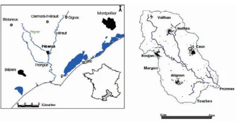
Fig. 1. Location of the study area
The studied spatial domain was the Peyne river catchment (75 km²) lo-cated in the mid Hérault valley in Languedoc-Roussillon, one of the world’s largest wine-producing regions (Figure 1). This catchment suffers from serious herbicide pollution of the surface water. Studies on the pollu-tion process show that this pollupollu-tion should be in relapollu-tionship with the high risk of herbicide leaching by run-off during the heavy rainfall events that are typical of the area’s sub-humid Mediterranean climate (Lennartz et al., 1997; Louchard et al., 2001). They assign a crucial role to the vineyard weed control practices (WCP), which determine both the type and amount of herbicide applied and the evolution of soil surface characteristics that
Version postprint
affect the soil’s hydraulic conductivity (Leonard and Andrieux, 1998; Hebrard et al., 2006).
The Peyne catchment incorporates all or part of the territories of eight local government areas (LGA, in France referred to as “communes”), and it is farmed by 650 winegrowers whose majority supply LGA-based coop-erative wineries.
3.2 Data
A geographical database was developed that included (a) information regarding WCP and (b) a description of physical or socio-economic vari-ables that can potentially explain the practices. The database contains a sample of 1007 geo-referenced vine plots of land, owned by 63 winegrow-ers and corresponding to 989 ha, i.e., about 20% of the area under vines within the Peyne valley.
Sampling scheme and data collection
The required data were gathered by surveying 63 winegrowers, selected by sampling plots along five transects perpendicular to the Peyne River. It was assumed that such a sampling adequately represented farm holdings and that the whole set of vine-plots of these farm holdings was representa-tive of the diversity and distribution of WCP in the valley.
The survey questionnaire focused on (1) the weed control practices used in each plot and (2) the variables assumed to explain the choice of prac-tices. In addition, the plots were precisely located on the land register map and the 1:100,000 soil map by Bonfils (1993).
Weed control practices
From the collected data, a 4-type expert-based stratification of the various WCP was performed regarding (1) their potential impact on surface runoff and (2) their intensity of herbicide use. Practice Pa is based on chemical weeding. In practice Pb, tillage alternates with chemical weed control in alleys. In practice Pc, the alleys are repeatedly shallow-tilled. In practice
Pd, tillage alternates with alleys under permanent grass.
From Pa to Pd (Pa > Pb >Pc > Pd), the environmental risk is less and less strong because of a reduction in herbicide amounts (from total to par-tial chemical weed control) and because of the use of weed control meth-ods that reduce more and more surface runoff.
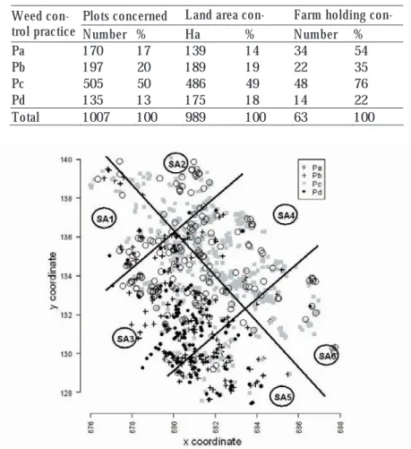
The survey results are resumed in table 1. They show that the most common practice over the entire catchment is Pc. When looking on the
Version postprint
sampled practice spatial distribution in figure 2, is clear that the WCP are not randomly distributed in space. Pc is the dominant practice on the left side of the Peyne River (on the right of the figure), whereas Pb and Pd are dominant on the right side of the river.
Table 1. Percentage of the different weed control strategies in the plots sample Plots concerned Land area con- Farm holding Weed
con-trol practice Number % Ha % Number %
Pa 170 17 139 14 34 54
Pb 197 20 189 19 22 35
Pc 505 50 486 49 48 76
Pd 135 13 175 18 14 22
Total 1007 100 989 100 63 100
Fig. 2. Spatial distribution of the observed practices (with division of the Peyne valley into six sub-areas (SA))
Explanatory variables
To generalize the prediction of WCP from explanatory variables (predic-tors) throughout the Peyne catchment, we tested only variables that can be easily collected from maps, remote sensing, or geo-referenced databases.
Version postprint
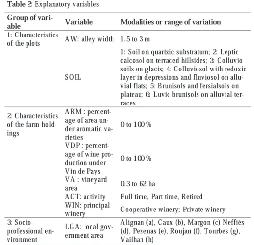
Table 2: Explanatory variables
Group of
vari-able Variable Modalities or range of variation
1: Characteristics
of the plots AW: alley width 1.5 to 3 m SOIL
1: Soil on quartzic substratum; 2: Leptic calcosol on terraced hillsides; 3: Colluvio soils on glacis; 4: Colluviosol with redoxic layer in depressions and fluviosol on allu-vial flats; 5: Brunisols and fersialsols on plateau; 6: Luvic brunisols on alluvial ter-races
2: Characteristics of the farm hold-ings
ARM : percent-age of area un-der aromatic va-rieties
0 to 100 % VDP :
percent-age of wine pro-duction under
Vin de Pays 0 to 100 % VA : vineyard
area 0.3 to 62 ha
ACT: activity Full time, Part time, Retired WIN: principal
winery Cooperative winery; Private winery 3:
Socio-professional en-vironment
LGA: local
gov-ernment area Alignan (a), Caux (b), Margon (c) Neffiès (d), Pezenas (e), Roujan (f), Tourbes (g), Vailhan (h)
Eight explanatory variables (predictors) were collected (table 2). These variables belong to three groups corresponding to three hypothesized lev-els of spatial organization of practices diversity: set 1, the physical charac-teristics of the plots (two variables), set 2, the structural characcharac-teristics and production priorities of the farm holdings (five variables), and set 3, the local government area (LGA) to which the plots belong. The choice of these three groups of variables was governed by the literature and the re-sults of a previous study conducted in two of the eight LGAs of the valley (Biarnès et al. 2004).
Version postprint
4. Results
4.1 Robust weed control practices classification trees
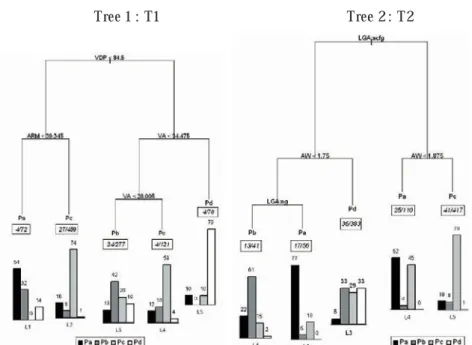
In a first step, robust trees were performed on two sets of explanatory vari-ables coming from the two main sources of available data (agricultural census or geographical databases). The tree T1 was performed on the set 2 of predictors (characteristics of the farm holdings) with a frequency pa-rameter f = 95 %. T2 was performed on the sets 1 and 3 of predictors (physical characteristics and socio-professional environment) with a fre-quency parameter f= 80 %. These parameters were selected to get at least four farms in each leaf. These trees are plotted in figure 3.
Tree 1 : T1 Tree 2 : T2
Fig. 3. Presentation of the selected robust trees. Each terminal node is associated (1) to a majority practice, (2) to an inset giving the number of farm holdings and the number of plots concerned, and (3) to a lay of distribution of the four modali-ties of WCP (% of plots).
When comparing the trees, T1 gives the most contrasted WCP distribu-tions (probabilities vectors) between leaves. It also presents, however, only strongly discriminant variables as shown by tree branch lengths that are re-lated to the discriminating power of the splitting variables. Only three
Version postprint
variables (VDP, VA, ARM) related to the economic scale and the produc-tive choices of the farm holdings are necessary to differentiate distribu-tions of practices. The right branch of the tree is associated with VDP ori-ented farm holdings (percentage of wine under VDP greater than 84 % of the total production). In these holdings, choices of practices vary according to the vine area. As a trend, winegrowers adopt practices that limit more and more polluting runoff (Pb, then Pc, then Pd) when increasing the vine area. In the farm holdings characterized by a weaker production of VDP (left branch of the tree), choices of weed control practices are linked to the percentage of area under aromatic varieties (ARM).
For the T2 tree, the root node is split on the values of the LGA variable, dividing the set of plots into two groups respectively located in the LGAs on the left side (right branch of the tree) and on the right side (left branch of the tree) of the Peyne River. The plots characterized by narrow alleys (AW less than 1.75 m or than 1.875 m according to the river side), are mainly associated with intensive use of herbicide (Pa, and even Pb). On the left side, the plots with wide alleys are mainly associated with practice
Pc, whereas they are equally associated to practices Pb,Pc, or Pd on the right side of the tree.
4.2 Assessment of spatial patterns resulting from robust tree predictions
In a second step, we used the robust calibrated trees T1 and T2 to simulate spatial distributions of WCP on the set of sampled vine plots.
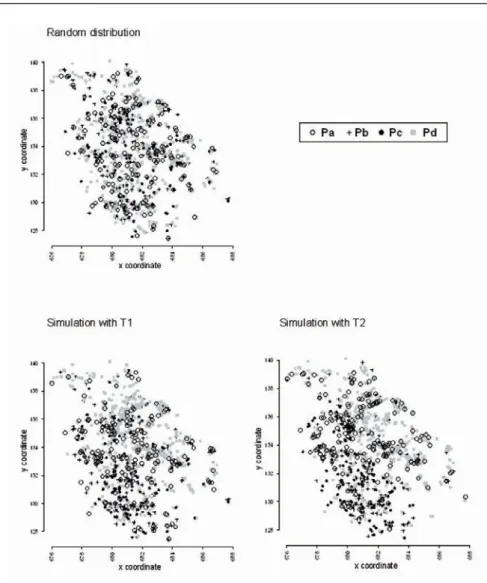
Figure 4 shows three examples of simulated WCP spatial distributions: a totally random spatial simulation respecting only global practices percent-ages in the top-left, a spatial simulation using tree T1 in the top-right, and a spatial simulation using tree T2 in the bottom-left. This figure shows that a random spatial distribution looks highly dissimilar to the observed one (Figure 2). Conversely, the stochastic use of trees gives contrasted and re-alistic distributions between the two sides of the Peyne River.
Version postprint
Fig. 4. Simulations of spatial distribution of practices
Global dissimilarities D between the observed WCP distributions and the n=1000 simulations were computed as explained in methods dividing the spatial domain into 6 cells (r=5 km, α=45°). These parameters were mainly chosen considering the two sides of the Peyne River. Computations were performed using successively trees T1, T2 and a totally random spa-tial simulation.
To obtain a distribution for these dissimilarities, this D computation was repeated 50 times, which yielded the statistics shown in table 3. Finally, the results show that simulations resulting from T2 are the closest to the
Version postprint
observed distribution even though T1 was the best based on a classical sta-tistical criteria (with purest leaves).
Table 3. Global dissimilarity distribution D between observed WCP spatial distri-bution and simulated ones
Dissimilarity statistics Aleatory distribution Tree 1 Tree 2
Mean 14.92 6.16 2.60
Quantile 98 % 15.27 6.23 2.64
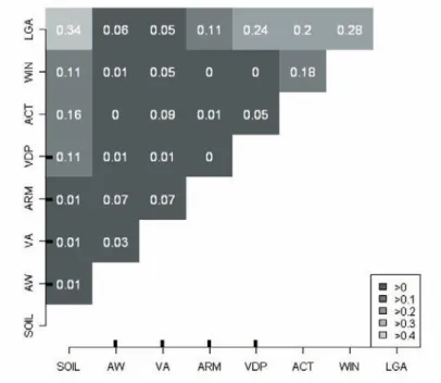
4.3 Interpreting tree results visualizing predictors correlation To better understand the latter result and the difference and similarities in trees T1 and T2, a square correlation matrix between all predictors was computed, as shown in table 4.
Table 4. Matrix of correlation statistics between variables. The four numerical variables have wide tickmarks on axes.
This table shows that the three groups of explanatory variables that we used are not entirely independent, and it highlights the role of the LGA
Version postprint
explanatory variable within the T2 tree. The plot variable SOIL and the holding variables VDP, WIN, and ACT are not randomly distributed among LGAs. Thus, LGA seemed to integrate various driving factors of practices, which explains its relevance in discriminating the practices: • In the case of VDP, this may be explained by the characteristics of the
wine production. This production is strongly governed by national regulations delimiting specific geographic areas for producing AOC or VDP wines (an AOC area is localized on three LGAs territories in the north-west of the Peyne Valley) and by the production orientations of the LGA-based wineries. Consequently, the LGAs of the Peyne catchment correspond to particular productive orientations of the farm holdings, which might explain the different practice distributions between LGAs.
• Correlation between SOIL and LGA comes from distinctive soil types over the Peyne Valley; LGA located on the right river side of the catchment have very clayey surface soils that almost do not exist in the LGA located on the other river side. These soils are part of the soils on the plateau described in table 2. They particularly justify the use of practicesPb or Pd due to the high risks of not having bearing capacity after a heavy rainfall event. The small area concerned by these soils does not justify by itself the extent of these practices, but studies on farm management showed an endeavour to simplify the work by limiting the range of different practices used (Aubry, 1998). A practice selected to resolve a particular problem in a particular plot may be used in other plots, which is the case with practices Pb and Pd.
• In addition, a leading role in the diffusion of practices by farm information networks has been shown by sociologists (Chiffoleau, 2005). The role of such networks and their links with LGA are being studied in two LGAs of the Peyne catchment by sociologists. Initial results showed that some of the winegrowers’ information networks (proximity networks, technical advice networks) might depend on the LGA where they are living and explain the differences in practices between LGAs. In particular, the use of practices Pb and Pd by winegrowers who do not have any plots in the very clayey soil area might be linked to the LGA-based proximity network to which these winegrowers belong.
Version postprint
5. Conclusion
In this paper, we presented and demonstrated the interest of an adaptation of a classification tree analysis that addresses current problems that are of-ten encountered with this method, especially when dealing with spatial data. We obtained robust trees that smooth the sampling sensitivity while keeping trees that look simple and that are easily interpretable. A specific evaluation procedure that considered the local spatial structures of the variable of interest was demonstrated to be useful when deciding between the candidate trees. Finally, the formulation of the correlations between the different variables helped to depict the complex role of a global variable (LGA) for explaining the observed spatial structure of agricultural prac-tices.
Other problems with the application of classification trees to spatial data will need to be addressed in the future. One suggestion is to be more ex-plicit about taking into account the autocorrelations of spatial data in tree-building algorithms as proposed by Bel et al (2005). Another suggestion is to consider the role of the uncertainty that affects both the explanatory variable and the variable to be explained, as pointed out by Lagacherie and Holmes (1997).
In this study, however, we developed a stochastic method that not only allows for simulation of the spatial distribution of the categorical variable in space but also gives a fully explicit view of the uncertainty associated with the classification process through the simulation of the spatial distri-bution of classes. Such an approach may further facilitate the assessment of model sensitivities to categorical variable map uncertainties when using these maps as input data in environmental impact assessment modelling.
References
Aaron, B., Kromrey, J. D., & Ferron, J. M. (1998). Equating r-based and d-based effect-size indices: Problems with a commonly recommended formula. An-nual meeting of the Florida Educational Research Association, Orlando, FL., ERIC Document Reproduction Service No. ED433353.
Aubry C., Papy F. and Capillon A. (1998). Modelling decision-making process for annual crop management. Agricultural Systems 56(1): 45-65.
Bel L., Laurent J.M. , Bar-Hen A., Allard D. and Cheddadi R. (2005). A spatial extension of CART: application to classification of ecological data, Geostatis-tics for environmental applications, Springer: Heidelberg, 99-109.
Version postprint
Biarnès A., Rio P. and Hocheux A. (2004). Analysing the determinants of spatial distribution of weed contol practices in a Languedoc vineyard catchment. Agronomie, 24: 187-191.
Bonfils P. (1993). Carte pédologique de France au 1/100°000 ; feuille de Lodève, SESCPF INRA.
Breiman L., Friedman J. H., Olshen R. A. and Stone C. J. (1984). Classification and Regression Tree. London, Chapman and Hall, 358 p.
Breiman L. (1996a). Bagging predictors. Machine learning 26(2): 123-140. Breiman L. (1996b). Random forest. Machine learning 45: 5-32.
Bui, E., and Moran, C. (2001). Disaggregation of polygons of superficial geology and soil maps using spatial modelling and legacy data. Geoderma, 103: 79-94. Chiffoleau Y. (2005). Learning about innovation through networks: the
develop-ment of environdevelop-ment-friendly viticulture. Technovation 25(10): 1193-1204. Cohen J. (1960). A coefficient of agreement for nominal scales, Educational and
Psychological Measurement 20: 37–46.
Espa, G., Benedetti, R., De Meo, A., U. Ricci and Espa S. (2006).GIS based models and estimation methods for the probability of archaeological site loca-tion, Journal of Cultural Heritage, 7(3), July,147-155
Fearer, T.M., Prisley, S.P., Stauffer; D.F., and Keyser P.D (2007). A method for integrating the Breeding Bird Survey and Forest Inventory and analysis data-bases to evaluate forest bird–habitat relationships at multiple spatial scales. Forest Ecology and Management, 243(1), 128-143
Gellrich, M., Baur, P., Robinson, B.H. and Bebi P. (2008). Combining classifica-tion tree analyses with interviews to study why sub-alpine grasslands some-times revert to forest: A case study from the Swiss Alps, Agricultural Systems, 96(1-3), 124-138
Geurts P., Ernst D. and Wehenkel L. (2006). Extremely randomized trees. Ma-chine learning 63: 3 - 42.
Gini C. (1912). Variabilità e mutabilità. Memorie di metodologica statistica. Vol. 1, E. Pizetti and T. Salvemini. Rome, Libreria Eredi Virgilio Veschi, pp 211-382
Goovaerts P. (2001). Geostatistical modelling of uncertainty in soil science. Ge-oderma 103: 3-26.
Haase, R.C. (1983). Classical and Partial Eta Square in Multifactor ANOVA De-signs. Educational and Psychological Measurement, 43(1), 35-39.
Hébrard O., Voltz M., Andrieux P. and Moussa R. (2006). Spatio-temporal distri-bution of soil surface moisture in a heterogeneously farmed Mediterranean catchment. Journal of Hydrology 329: 110-121.
Ihaka R. and Gentleman R. (1996). R: A Language for Data Analysis and Graph-ics,.Journal of Computational and Graphical Statistics 5(3): 299-314. Lagacherie, P. and Holmes, S. (1997). Addressing geographical data errors in a
classification tree for soil unit prediction. Int. J. Geographical Info. Sci. 11, pp. 183–198
Lennartz B., Louchard X., Voltz M. and Andrieux P. (1997). Diuron and simazine losses to runoff water in mediterranean vineyards. Journal of Environmental Quality 26(6): 1493-1502.
Version postprint
Leonard J. and Andrieux P. (1998). Infiltration characteristics of soils in Mediter-ranean vineyards in Southern France. Catena 32: 209-223.
Louchart X., Voltz M., Andrieux P. and Moussa R. (2001). Herbicide Transport to Surface Waters at Field and Watershed Scales in a Mediterranean Vineyard Area. Journal of Environmental Quality 30: 982-991.
McDonald, R.I., Urban, D.L. (2006). Spatially varying rules of landscape change: lessons from a case study, Landscape and Urban Planning, 74(1), 7-20. Mahalanobis P. C. (1936). On the generalised distance in statistics. Proceedings of
the National Institute of Science of India 12: 49-55.
Ripley B. (2007). Pattern recognition and neural Networks. Cambrige, Cambridge University Press, 415 p.
Schröder W., (2006). GIS, geostatistics, metadata banking, and tree-based models for data analysis and mapping in environmental monitoring and epidemiology, International Journal of Medical Microbiology, Volume 296(1-22 ), 23-36. Tittonell, P., Shepherd, K.D. , Vanlauwe, B. and Giller, K.E. (2008) Unravelling
the effects of soil and crop management on maize productivity in smallholder agricultural systems of western Kenya—An application of classification and regression tree analysis, Agriculture, Ecosystems & Environment, 123(1-3), 137-150.