CoMapping: Efficient 3D-Map Sharing Methodology for Decentralized cases

HAL Id: hal-01867720

https://hal.archives-ouvertes.fr/hal-01867720

Submitted on 4 Sep 2018

HAL is a multi-disciplinary open access

archive for the deposit and dissemination of

sci-entific research documents, whether they are

pub-lished or not. The documents may come from

teaching and research institutions in France or

abroad, or from public or private research centers.

L’archive ouverte pluridisciplinaire HAL, est

destinée au dépôt et à la diffusion de documents

scientifiques de niveau recherche, publiés ou non,

émanant des établissements d’enseignement et de

recherche français ou étrangers, des laboratoires

publics ou privés.

CoMapping: Efficient 3D-Map Sharing Methodology for

Decentralized cases

Luis Contreras-Samamé, Salvador Dominguez-Quijada, Olivier Kermorgant,

Philippe Martinet

To cite this version:

Luis Contreras-Samamé, Salvador Dominguez-Quijada, Olivier Kermorgant, Philippe Martinet.

CoMapping: Efficient 3D-Map Sharing Methodology for Decentralized cases. 10th workshop on

Plan-ning, Perception and Navigation for Intelligent Vehicles at Int. Conf. on Intelligent Robots and

Systems, Oct 2018, Madrid, Spain. �hal-01867720�

CoMapping: Efficient 3D-Map Sharing

Methodology for Decentralized cases

Luis F. Contreras-Samam´e, Salvador Dom´ınguez-Quijada, Olivier Kermorgant and Philippe Martinet

∗_{INRIA Sophia Antipolis, 06902 Sophia Antipolis, France}

Emails: Luis.Contreras@ls2n.fr, Salvador.Dominguezquijada@ls2n.fr, Olivier.Kermorgant@ls2n.fr, Philippe.Martinet@inria.fr

Abstract—CoMapping is a framework to efficient manage, share, and merge 3D map data between mobile robots. The main objective of this framework is to implement a Collaborative Mapping for outdoor environments. The framework structure is based on two stages. During the first one, the Pre-Local Mapping stage, each robot constructs a real time pre-local map of its environment using Laser Rangefinder data and low cost GPS information only in certain situations. Afterwards, the second one is the Local Mapping stage where the robots share their pre-local maps and merge them in a decentralized way in order to improve their new maps, renamed now as local maps. An experimental study for the case of decentralized cooperative 3D mapping is presented, where tests were conducted using three intelligent cars equipped with LiDAR and GPS receiver devices in urban outdoor scenarios. We also discuss the performance of the cooperative system in terms of map alignments.

I. INTRODUCTION

Mapping the environment can be complex since in certain situations, e.g. in large regions, it may require a group of robots that build the maps in a reasonable amount of time with regards to the expected accuracy [1]. A set of robots extends the capability of a single robot by merging measurements from group members, providing each robot with information beyond their individual sensors range. This leads to a better usage of resources and execution of tasks which are not feasible by a single robot. Multi-robot mapping is considered as a centralized approach when it requires all the data to be analysed and merged at a single computation unit. Otherwise, in a decentralized approach, each robot builds their local maps independent of one another and merge their maps upon rendezvous.

Individual Pre-Local &

Local Mapping FLUENCE Renault

Individual Pre-Local &

Local Mapping ZOE Renault

Shared data

Individual Pre-Local &

Local Mapping GOLFCAR

Shared data

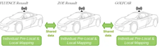
Fig. 1. Scheme of our CoMapping System considering a decentralized case

Figure 1 depicts the scheme of work proposed in this article for a group of robots where it was assumed that ZOE robot have direct exchange of data (as pose, size and limits of maps) with FLUENCE and GOLFCAR. And by contrast, FLUENCE and GOLFCAR are in a scenario of non-direct communication,

with limited access conditions to a same environment, and without any meeting point for map sharing between these mobile units.

Following this scenario, this paper presents the development and validation of a new Cooperative Mapping framework (CoMapping) where:

• In the first stage named “Pre-Local Mapping”, each individual robot builds its map by processing range measurements from a 3D LiDAR moving in six de-grees of freedom (6-DOF) and using low cost GPS data (GPS/GGA).

• For the second stage named “Local Mapping”, the robots

send a certain part of their pre-local maps to the other robots based on our proposed Sharing algorithm. The registration process includes an intersecting technique of maps to accelerate processing.

This work is addressed to outdoor environments applications denied of a continuous GPS service by using a decentralized approach. Our proposal has been tested and validated in an outdoor environment, with data acquired on the surroundings of the ECN ( ´Ecole Centrale Nantes) campus.

II. RELATED WORKS

In a scenario of cooperative mapping, robots first operate independently to generate individual maps. Here the regis-tration method plays a fundamental role. Many regisregis-tration applications use LiDAR as a Rangefinder sensor for map building [2]. However, a high Lidar scan rate can be harmful for this task, since it may create distortion in the map con-struction. For those cases, ICP approaches [3] can be applied to match different scans. Implementations, for 2 or 3-axis and geometric structures matches of a generated local point set, were presented in [4] [5]. Those methods use batch processing to build maps offline. In the first stage of our implementation we reconstruct maps as 3D point clouds in real-time using 3-axis LiDAR by extraction and matching of geometric features in Cartesian space based in [6]. Then our system uses GPS position data to coarsely re-localize that cloud in a global frame.

Once all the maps have been projected on a global frame, they have to be merged together to form a global map. In this context, [7] proposed a method for 3D merging of occupancy grid maps based on octrees [8] for multi-robots.

The method was validated in a simulation environment. For the merging step, an accurate transformation between maps was assumed as known, nevertheless in real applications, that information is not accurate, since it is obtained by means of uncertain sensor observations. In our case, real experiments were performed for a multi-robot application without perfect knowledge of the transformations between the maps. In [9] a pre-merging technique is proposed, which consists in selecting the subset of points included in the common region between maps bounding. Then, a centralized merging process refines the transformation estimate between maps by ICP registration [3]. We use a variation of [9] but previously we include an efficient technique to exchange maps between robots in order to optimize bandwidth.

Other solutions may be used in order to merge maps for a group of robots with a centralized approach [10], [9], [11], which are generally found in the literature. However this kind of solutions can compromise the team performance because merging and map construction depend exclusively on a processing unit. Another approach less explored and analysed is the decentralized one [12], [1], [13]. The advantage in this case lies in the independence and robustness of the system because map construction is not affected even if one of the robots has failures in communication or processing, since map merging can be executed in different units after traversing the environment. This kind of approach can consider a meeting point for the vehicles in order to exchange their maps and other data. This approach is also investigated in our final experiments.

III. METHODOLOGY

A. Pre-Local Mapping Stage

Each mobile robot executes a Pre-Local Mapping system using data provided by a LidarSLAM process. We just use coarse GPS position to project the generated map on a global frame. In order to reduce implementation costs, a beneficial cheap GPS service was used, specifically GPS/GGA (Global Positioning System Fix Data) at an accuracy of about 2 to 7 meters. Another advantage of our Pre-Local Mapping Stage is its versatile configuration, since it does not depend on a specific LidarSLAM method.

A modified version of the LOAM technique1 _{[6] was thus}

chosen as the LidarSLAM method for this work.

Pose of 1st frame from 10Hz Transform 1Hz Undistorted Point Cloud Registration Lidar Lidar

Odometry MappingLidar

GPS data

1Hz Pre-Local Map Output LidarSLAM

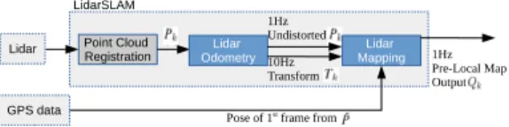
Fig. 2. Architecture of Pre-Local Mapping Stage

Figure 2 illustrates the block diagram of this stage, where ˆ

P is the raw point cloud data generated by a laser scanner in the beginning. The accumulated point cloud up to sweep k

1_{LOAM: https://github.com/laboshinl/loam velodyne}

is denoted Pk and processed by a Lidar Odometry algorithm,

which runs at a frequency around 10Hz and computes the lidar motion (transform Tk) between two consecutive sweeps. The

distortion in Pk is corrected using the estimated lidar motion.

The resulting undistorted Pk is processed at a frequency of

1Hz by an algorithm knows as Lidar Mapping, which performs the matching and registration of the undistorted cloud onto a map. Using the GPS information of the vehicle pose, it is possible to coarsely project the map of each robot into common coordinate frame for all the robots. This projected cloud is denoted as the Pre-Local Map.

1) Lidar Odometry step: The step begins with feature points extraction from the cloud Pk. The feature points are

selected from sharp edges and planar surface patches. Let us define S as the set of consecutive points i returned by the laser scanner in the same scan, where i ∈ Pk. An indicator

proposed in [6] evaluates the smoothness of the local surface as following: c = 1 | S | . k XL (k,i)k k X j∈S,j6=i (X_(k,i)L − XL (k,j)) k, (1)

where X_(k,i)L and X_(k,j)L are the coordinate of two points from the set S.

Moreover, a scan is split into four subregions to uniformly distribute the selected feature points within the environment. In each subregion is determined maximally two edge points and four planar points. The criteria to select the feature points as edge points is related to maximum c values, and by contrast the planar points selection to minimum c values. When a point is selected, it is thus mandatory that none of its surrounding points are already selected. Besides, selected points on a surface patch cannot be approximately parallel to the laser beam, or on boundary of an occluded region.

When the correspondences of the feature points are found, then the distances from a feature point to its correspondence are calculated. Those distances are named as dE and dH for

edge points and planar points respectively. The minimization of the overall distances of the feature points leads to the Lidar odometry. That motion estimation is modeled with constant angular and linear velocities during a sweep.

Let us define Ek+1and Hk+1as the sets of edge points and

planar points extracted from Pk+1, for a sweep k+1. The lidar

motion relies on establishing a geometric relationship between an edge point in Ek+1and the corresponding edge line:

fE(X(k+1,i)L , T L

k+1) = dE, i ∈ Ek+1, (2)

where T_k+1L is the lidar pose transform between the starting time of sweep k + 1 and the current time ti. Analogously,

the relationship between a planar point in Hk+1 and the

corresponding planar patch is: fH(X(k+1,i)L , T

L

Equations (2) and (3) can be reduced to a general case for each feature point in Ek+1 and Hk+1, leading to a nonlinear

function:

f (T_k+1L ) = d, (4)

in which each row of f is related to a feature point, and d possesses the corresponding distances. Levenberg-Marquardt method [14] is used to solve the Equation (4). Jacobian matrix (J) of f with respect to T_k+1L is computed. Then, the minimization of d through nonlinear iterations allows solving the sensor motion estimation:

T_k+1L ←− TL k+1− (J

T

J + λdiag(JTJ))−1JTd, (5) where λ is the Levenberg-Marquardt gain.

Finally, the Lidar Odometry algorithm produces a pose transform T_k+1L that contains the lidar tracking during the sweep between [tk+1 , tk+2] and simultaneously an

undis-torted point cloud ¯Pk+1. Both outputs will be used by the

Lidar Mapping step, detailed in the next section.

2) Lidar Mapping step: This algorithm is used only once per sweep and runs at a lower frequency (1 Hz) than the Lidar Odometry step (10 Hz). The technique matches, registers and projects the cloud ¯Pk+1provided by the Lidar Odometry as a

map into the coordinate system of a vehicle, noted as {V }. To understand the technique behaviour, let us defined Qk as the

point cloud accumulated until sweep k, and TV

k as the sensor

pose on the map at the end of sweep k, tk+1. The algorithm

extends TV

k for one sweep from tk+1 to tk+2, to get Tk+1V ,

and projects ¯Pk+1on the robot coordinate system, denoted as

¯

Qk+1. Then, by optimizing the lidar pose Tk+1V , the matching

of ¯Qk+1 with Qk is obtained.

In this step the feature points extraction and their correspon-dences are calculated in the same way as in Lidar Odometry, the difference just lies in that all points in ¯Qk+1share the time

stamp, tk+2.

In that context, nonlinear optimization is solved also by the Levenberg-Marquardt method [14], registering ¯Qk+1on a new

accumulated cloud map. To get a uniform points distribution, down-sampling is performed to the cloud using a voxel grid filter [15] with a voxel size of 5 cm cubes.

Finally, since we have to work with multiple robots, we use a common coordinate system for their maps, {W }, coming from rough GPS position estimation of the 1st accumulated cloud frame Qk.

B. Local Mapping Stage

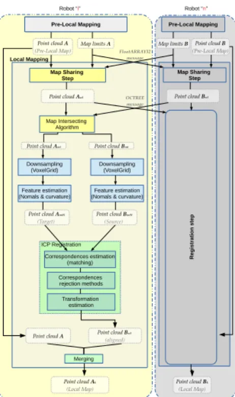
In this section the Local Mapping is detailed, considering that the process is executed on the robot “i” with a shared map by robot “n” (see Figure 3).

1) Map Sharing Step: When the generation of Pre-Local Maps is done, the robots would have to exchange their maps to start the map alignment process. In several cases the sharing and processing of large maps can affect negatively the performance of the system with respect to runtime and

Robot “i”

Downsampling (VoxelGrid) Feature estimation (Nomals & curvature)

Downsampling (VoxelGrid) Feature estimation (Nomals & curvature)

Correspondences rejection methods Transformation estimation ICP Registration Map Intersecting Algorithm Map Sharing Step Robot “n” Local Mapping Map limits A Point cloud A (Pre-Local Map)

Point cloud Asel

Point cloud A Point cloud Bsel (aligned) Correspondences estimation (matching) Point cloud AL (Local Map) Pre-Local Mapping Merging

Pre-Local Mapping Pre-Local Mapping

Map limits B_{(Pre-Local Map)}Point cloud B

Point cloud BL

(Local Map)

Point cloud Aint Point cloud Bint

Point cloud AintN (Target)

Point cloud BintN (Source) OCTREE message FloatARRAY32 message R e g is tr a ti o n s te p Map Sharing Step

Point cloud Bsel

Fig. 3. Architecture of Local Mapping Stage for one robot “i”, receiving

map data from another robot “n”. Pre-Local Map

from robot ”i”: Point cloud A Pre-Local Map from robot ”i”: Point cloud A Pre-Local Map from robot ”n”: Point cloud B Pre-Local Map from robot ”n”: Point cloud B Sharing Region (automatic adjustment)Sharing Region (automatic adjustment) Aminx Aminx Amaxx Amaxx Bminx

Bminx CCxx BmaxBmaxxx

Cy Cy C C L L L L L L LL Linit Linit

Fig. 4. Graphical representation of the Map Sharing technique (Top view

of plane XY). Aminx, Amaxx, Bminx and Bmaxx represent the point

cloud limits along the x-axis.

memory usage. A sharing technique is presented in order to overcome this problem, in which each vehicle only sends a certain subset of points of its map to the other robots. When the maps are ready for transferring, they are compressed in octree format using OctoMap library [8] in order to optimize the robot-communication.

The proposed sharing technique is based on the method developed in [16]. Figure 4 depicts the behaviour, wherein point clouds A and B represent the Pre-Local Maps from two robots “i” and “n” respectively. In each robot the algorithm first receives only information about the 3D limits of the maps (i.e. bounding cubic lattice of the point clouds) and then

decides what part of its map will be shared to the other robot. These limits were determined previously using the function GetBounds() that returns two vectors: in the first one, Amin, their components represent the lowest displacement from the origin along each axis in the point cloud; and the other vector, Amax, is related to the point of the highest displacement.

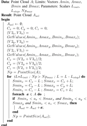
Algorithm 1: Selection of Point Cloud to share with another robot.

Pseudo-code of the map sharing step is described in Al-gorithm 1. Inside the code, the function GetV alues() sorts in ascending order the array of components along each axis of the vectors Amin, Amax, Bmin, Bmax and returns the 2nd and 3rd values from this sorted array, denoted V 2 and V 3 respectively. Then for each axis, the average of the two values obtained by the function GetV alues() is used in order to determine the Cartesian coordinate (Cx,Cy,Cz)

of the geometric center of the sharing region S. This map sharing region is a cube whose edge length 2L is determined iteratively. The Points from A contained in this cube region are extracted to generate a new point cloud Asel. In each iteration

the cube region is reduced until the number of points from Asel

is smaller than the manual parameter N pmax, which represents

the number of points maximum that the user wants to exchange between robots. Once the loop ends, Asel is sent to the other

robot. Analogously on the other mobile robot “n”, the points from B included in this region are also extracted to obtain and share Bsel with the another robot “i”. Finally, the clouds

Aseland Bselare encoded and sent in octree format to reduce

the usage of bandwidth resources of the multi-robot network. Then maps are decoded and reconverted in 3D point cloud format to be used in the Registration step.

2) Registration Step: The intersecting volumes of the two maps Asel and Bsel are computed and denoted as Aint and

Bint, obtained from the exchanged map bounds [9]. In order to

improve the computation speed, point clouds Aintto Bintfirst

go through a down-sampling process to reduce the number of points in the cloud alignment. Feature descriptors as surface normals and curvature are used to improve the matching, which is the most expensive stage of the registration algorithm [17]. These generated normal-point clouds AintN and BintN

are then used by Iterative Closest Point (ICP) algorithm [18]. This method refines an initial alignment between clouds, which basically consists in estimating the best transformation to align a source cloud BintN to a target cloud AintN by iterative

minimization of an error metric function. At each iteration, the algorithm determines the corresponding pairs (b’, a’), which are the points from AintN and BintN respectively, with the

least Euclidean distance.

Then, least squares registration is computed and the mean squared distance E is minimized with regards to estimated translation t and rotation R:

E(R, t) = 1 N pb’ N pb’ X i=1 k a’i− (R b’i+ t) k 2 , (6)

where N pb0 is the number of points b’.

The resulting rotation matrix and translation vector can be express in a homogeneous coordinate representation (4×4 transformation matrix Tj) and are applied to BintN. The

algorithm then re-computes matches between points from AintN and BintN, until the variation of mean square error

between iterations is less than a defined threshold. The final ICP refinement for n iterations can be obtained by multiplying the individual transformations: TICP = Q

n

j=1Tj. Finally the

transformation TICP is applied to the point cloud Bselto align

and merge with the original point cloud A, generating the Lo-cal Map ALthen. Each robot thus performed its own merging

according to data from other agents within communication range. We now present the corresponding experimental results.

IV. RESULTS

Fig. 5. Vehicles used in the tests: ZOE, FLUENCE and GOLFCAR.

In this section we show results validating the presented concepts and the functionality of our system. As we consider ground vehicles, the ENU (East-North-Up) coordinate system is used as external reference of the world frame {W }, where y-axis corresponds to North and x-axis corresponds to East,

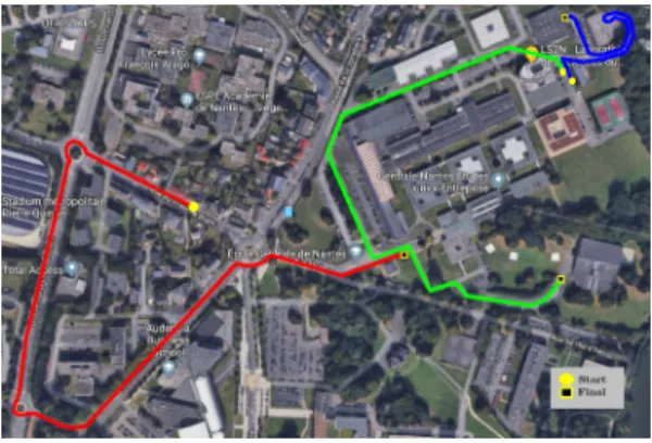
Fig. 6. Paths followed by ZOE (green one), FLUENCE (red one) and GOLFCAR robot (blue one) during experiments. Image source: Google Earth.

but coinciding its origin with the GPS coordinate [Longitude: -1.547963; Latitude: 47.250229].

The proposed framework is validated considering three vehicles for experiments, a ZOE Renault, a FLUENCE Renault and a GOLFCAR (see Figure 5) customized and equipped with a Velodyne VLP-16 3D LiDAR, with 360◦horizontal and a 30◦ vertical field of view. All data come from the campus outdoor environment in an area of approximately 1000m x 700m. The vehicles traversed that environment following different paths and collected sensor observations about the world, running pre-local mapping process in real-time.

For the validation, the vehicles build clouds from different paths (see Figure 6). Results of the Pre-Local Mapping of this experiment are shown in Figure 7.

Fig. 7. Top view of unaligned Pre-Local Maps generated by ZOE (green

one), FLUENCE (red one) and GOLFCAR robot (blue one) projected on common coordinate system

Figure 7 also depicts the “sharing region” determined during the map exchange process in each robot. It was assumed that all the vehicles have the constraint of exchanging a maximum number of points N pmaxof 410000 to simulate restrictions in

resources of bandwidth network or memory usage in robots. The tests were divided in two. In the first one, test A, ZOE and FLUENCE car define a meeting point to transfer their maps. Around this position, ZOE car exchanges and updates its local map and then a new point of rendezvous for map sharing is determined by ZOE and GOLFCAR in the following test B.

As we assume a decentralized scenario, each robot performs a relative registration process considering its Pre-Local map as target cloud for alignment reference. Each vehicle also executes the intersecting algorithm and then an ICP refinement to obtain an improved transform between each map. Figures 8 and 9 depict in yellow color the intersection between the shared point clouds during the alignment process. Once the refined transformation is obtained, it is then applied to the shared map.

Fig. 8. Test A: Alignment of the intersecting regions with ICP refinement

performed in ZOE robot, when it received the FLUENCE map (a) Green and red maps represent the target and source clouds pre ICP, top view (b) Green and blue maps represent the target and aligned source clouds post ICP, top view. Alignment can be better appreciated in yellow box

Fig. 9. Test B: Alignment of the intersecting regions with ICP refinement

performed in ZOE robot, when it received the GOLFCAR map (a) Green and red maps represent the target and source clouds pre ICP, top view (b) Green and blue maps represent the target and aligned source clouds post ICP, top view. Alignment can be better appreciated in yellow box

Quantitative alignment results of the ICP transformation relative to each robot are shown in Tables I and II. All the ICP transformations are expressed in Euler representation (x, y, z, roll, pitch, yaw) in meters and radians. The first row of Table I corresponds to the merging process in ZOE, when this robot received the map shared by FLUENCE and it aligned that map to its own pre-local map. The decentralized system demonstrated alignments in opposite directions for both robots, since each robot performs the merging process considering its Pre-Local map as target cloud for alignment reference. Table II also reveals this symmetrical behavior, where the algorithm on ZOE converged to the value of displacement of -0.1782 m and -3.2605 m along the x-axis and y-axis respectively. On the other hand on the GOLFCAR robot, the algorithm converged to a value of displacement of 0.2213 m and 3.3857 m along the x-axis and y-axis respectively, reconfirming relative alignments in opposite directions.

Figure 10 shows one of the merging results corresponding to the ZOE robot, in which the cloud represents the final

TABLE I

TESTA: RELATIVEICPTRANSFORMATIONS INEULER FORMAT BETWEEN

ZOEANDFLUENCEROBOT

Robot x y z roll pitch yaw

ZOE -1.6517 3.0966 -9.9729 0.0132 0.0730 0.0022

FLU. 4.5748 -4.4556 6.6061 -0.0054 -0.0624 -0.0084

TABLE II

TESTB: RELATIVEICPTRANSFORMATIONS INEULER FORMAT BETWEEN

ZOEANDGOLFCARROBOT

Robot x y z roll pitch yaw

ZOE -0.1782 -3.2605 1.7771 -0.0516 0.0115 0.0356

GOL. 0.2213 3.3857 -2.6070 0.0411 -0.0256 -0.0380

Fig. 10. Top view of final 3D Local Map of ZOE robot (color). Uniform

green point clouds come from the aligned maps of FLUENCE (left) and GOLFCAR (right)

3D local map projected on a 2D map in order to make qualitative comparisons. Experiments showed the impact of working with intersecting regions, since it can accelerate the alignment process by decreasing the number of points to compute. In the same way, tests demonstrated that our proposed map sharing technique developed a transcendental position in the performance of the entire mapping collaborative system by reducing the map size to transmit. Finally, the sharing algorithm proves to be a suitable candidate to exchange efficiently maps between robots considering the use of clouds of large dimensions.

V. CONCLUSION ANDFUTURE WORK

A framework was presented for decentralized 3D mapping system for multiple robots. The work has showed that maps from different robots can be successfully merged, from a coarse initial registration and a suitable exchange of data volume. The system uses initially range measurements from a 3D LiDAR, generating a pre-local maps for each robot. The complete system solves the mapping problem in an efficient and versatile way that can run in computers dedicated to three vehicles for experiments, leading to merge maps independently on each vehicle for partially GPS-denied environments. Future work will focus on the analysis of the consistency of the final maps estimated on each robots

ACKNOWLEDGMENT

This article is based upon work supported by the Erasmus Mundus Action 2 programme through the Sustain-T Project. The authors also gratefully acknowledge all the members of ECN, LS2N and INRIA institution on this work. Parts of the equipments used here were funded by the project ROBOTEX, reference ANR-10-EQPX-44-01.

REFERENCES

[1] P. Dinnissen, S. N. Givigi, and H. M. Schwartz, “Map merging of

multi-robot SLAM using reinforcement learning.” in SMC. IEEE,

2012. [Online]. Available: http://dblp.uni-trier.de/db/conf/smc/smc2012. html#DinnissenGS12

[2] S. Kohlbrecher, O. V. Stryk, T. U. Darmstadt, J. Meyer, and U. Klingauf, “A flexible and scalable SLAM system with full 3D motion estimation,” in in International Symposium on Safety, Security, and Rescue Robotics. IEEE, 2011.

[3] F. Pomerleau, F. Colas, R. Siegwart, and S. Magnenat, “Comparing ICP variants on real-world data sets - open-source library and experimental protocol.” Auton. Robots, 2013. [Online]. Available: http://dblp.uni-trier. de/db/journals/arobots/arobots34.html#PomerleauCSM13

[4] R. Zlot and M. Bosse, “Efficient Large-Scale 3D Mobile Mapping and Surface Reconstruction of an Underground Mine.” in FSR, ser. Springer Tracts in Advanced Robotics, K. Yoshida and S. Tadokoro,

Eds. Springer, 2012. [Online]. Available: http://dblp.uni-trier.de/db/

conf/fsr/fsr2012.html#ZlotB12

[5] M. Bosse, R. Zlot, and P. Flick, “Zebedee: Design of a Spring-Mounted 3-D Range Sensor with Application to Mobile Mapping,” IEEE Transactions on Robotics, Oct 2012.

[6] J. Zhang and S. Singh, “LOAM: Lidar odometry and mapping in real-time,” in Robotics: Science and Systems, 2014.

[7] J. Jessup, S. N. Givigi, and A. Beaulieu, “Merging of octree based 3D occupancy grid maps,” in 2014 IEEE International Systems Conference Proceedings, March 2014.

[8] A. Hornung, K. M. Wurm, M. Bennewitz, C. Stachniss, and W. Burgard, “OctoMap: An Efficient Probabilistic 3D Mapping Framework Based on Octrees,” Auton. Robots, Apr. 2013. [Online]. Available: http://dx.doi.org/10.1007/s10514-012-9321-0

[9] J. Jessup, S. N. Givigi, and A. Beaulieu, “Robust and Efficient Mul-tirobot 3-D Mapping Merging With Octree-Based Occupancy Grids,” IEEE Systems Journal, 2015.

[10] A. Birk and S. Carpin, “Merging occupancy grid maps from multiple robots,” Proceedings of the IEEE, July 2006.

[11] R. Dub´e, A. Gawel, H. Sommer, J. Nieto, R. Siegwart, and C. Ca-dena, “An online multi-robot SLAM system for 3D LiDARs,” in 2017 IEEE/RSJ International Conference on Intelligent Robots and Systems (IROS), Sept 2017, pp. 1004–1011.

[12] N. E. ¨Ozkucur and H. L. Akin, “Supervised feature type selection

for topological mapping in indoor environments,” in 21st Signal Processing and Communications Applications Conference, SIU 2013, Haspolat, Turkey, April 24-26, 2013, 2013, pp. 1–4. [Online]. Available: http://dx.doi.org/10.1109/SIU.2013.6531556

[13] J. Zhang and S. Singh, “Aerial and Ground-based Collaborative Map-ping: An Experimental Study,” in The 11th Intl. Conf. on Field and Service Robotics (FSR), Sep 2017.

[14] R. I. Hartley and A. Zisserman, Multiple View Geometry in Computer Vision, 2nd ed. Cambridge University Press, ISBN: 0521540518, 2004. [15] R. Rusu and S. Cousins, “3D is here: Point Cloud Library (PCL),” in Robotics and Automation (ICRA), 2011 IEEE International Conference on, May 2011.

[16] L. Contreras, O. Kermorgant, and P. Martinet, “Efficient Decentralized Collaborative Mapping for Outdoor Environments,” in 2018 IEEE Inter-national Conference on Robotic Computing (IRC), Laguna Hills, United States, Jan 2018 - In Press.

[17] S. Rusinkiewicz and M. Levoy, “Efficient variants of the ICP algorithm,” in Third International Conference on 3D Digital Imaging and Modeling (3DIM), Jun. 2001.

[18] P. J. Besl and N. D. McKay, “A Method for Registration of 3-D Shapes,” IEEE Trans. Pattern Anal. Mach. Intell., Feb. 1992. [Online]. Available: http://dx.doi.org/10.1109/34.121791