An analytic nodal method for solving the two-group, multidimensional, static and transient neutron diffusion equations

AN ANALYTIC NODAL METHOD

FOR SOLVING THE TWO-GROUP, MULTIDIMENSIONAL, STATIC AND TRANSIENT NEUTRON DIFFUSION EQUATIONS

by

Kord S. Smith

B. S. , Kansas State University ( 1976)

SUBMITTED IN PARTIAL FULFILLMENT OF THE REQUIREMENTS FOR THE

DEGREES OF NUCLEAR ENGINEER

AND

MASTER OF SCIENCE AT THE

· @

.

Signature redacted

Signature of Author. • . • . . . ,, , .v . - ~ • Y\J < •. ...- -. • -... • • • • •

Department of Nuclear Engineering, March /Cf, 19 79

Signature redacted

Certified by • • • • ...,,,.. • , • r • . • •

-·v..,./. . . .

Signature redacted

AN ANALYTIC NODAL METHOD

FOR SOLVING THE TWO-GROUP, MULTIDIMENSIONAL, STATIC AND TRANSIENT NEUTRON DIFFUSION EQUATIONS

by

Kord S. Smith

Submitted to the Department of Nuclear Engineering on March 9, 1979, in partial fulfillment of the requirements for the Degrees of Nuclear Engineer and Master of Science.

ABSTRACT

The objective of this research is to develop computationally effi-cient numerical methods for solving the two-group, multidimensional, static and transient neutron diffusion equations. In particular, refine-ments of the Analytic Nodal Method (which employs analytic solutions of the one-dimensional diffusion equations to determine spatial coupling) are investigated.

In the static case, the only approximation of the Analytic Nodal

ehd-isthat-thespatial-shape-of-thetransverse-JnkageS-Canhe~fit-quadratic polynomials. Numerical techniques for solving the nodal dif-fusion equations are investigated and optimized for LWR analysis with assembly-sized spatial mesh. The nodal method is extended to the time-dependent case by use of the Theta time-integration method.

Analysis of many two- and three-dimensional, static and transient LWR problems demonstrates that very accurate solutions can be

obtained with assembly-sized spatial meshes (15-20 cm). The computa-tional efficiency of the Analytic Nodal Method is also shown to be at least two orders of magnitude greater than that of conventional finite difference methods.

Thesis Supervisor: Allan F. Henry Title: Professor of Nuclear Engineering

ACKNOWLEDGMENTS

The author extends his sincerest appreciation to his thesis supervisor, Professor Allan F. Henry, for his invaluable assistance and support during the course of this investigation. His unique ability to motivate and direct his students, while providing ample opportunity

for development and exploration of his students' ideas, has made the author's association with him an extremely rewarding experience.

Thanks are also due to Professor Kent F. Hansen for his helpful comments on certain numerical considerations of this work.

The author also wishes to thank Mrs. Mary Bosco for her assist-ance in the preparation of this document. Her patience and technical skills, which are clearly demonstrated in this manuscript, are only exceeded by the apparent pride which she places in her work. The author is grateful for all her laborious efforts.

The financial support of this research by the Electric Power Research Institute is gratefully acknowledged.

TABLE OF CONTENTS Page Abstract Acknowledgments iii List of Figures ix List of Tables xi Chapter 1. INTRODUCTION 1-1 1. 1 Overview 1-1

1. 2 Synopsis of the Problem 1-3

1.3 Review of Solution Methods 1-6

1.4 Motivation of Nodal Methods 1-10

1.5 Objectives and Summary 1-10

Chapter 2. DERIVATION OF THE ANALYTIC NODAL METHOD FOR SOLVING THE STATIC MULTIGROUP

DIFFU-SION EQUATIONS 2-1

2.1 Introduction 2-1

2.2 Derivation of Three-Dimensional Multigroup

Nodal Diffusion Equations 2-2

2. 3 Derivation of Spatial Coupling Equations 2-6 2. 3. 1 The "Buckling" Approximation 2-8 2. 3. 2 The "Flat" Approximation 2-9 2. 3. 3 The "Quadratic" Approximation 2-10 2.4 Method for Solving the Spatial Coupling Equations

with Quadratic Transverse Leakage 2-11

Page

Chapter 3. NUMERICAL CONSIDERATIONS 3-1

3.1 Introduction 3-1

3. 2 Numerical Properties of the Analytic Nodal

Diffusion Equations 3-1

3. 3 Iterative Strategy for Solving the Static Nodal

Diffusion Equations 3-7

3. 3. 1 The General Iterative Scheme 3-7

3. 3. 2 Eigenvalue Updating 3-8

3. 3. 3 Outer Iterations 3-9

3.3.4 Inner Iterations 3-12

3. 3. 5 Flux Iterations 3-13

3.4 Iteration Optimization 3-17

3.4. 1 Flux Iteration Error Reduction 3-18 3. 4. 2 Eigenvalue Shift Optimization 3-19

3.5 Summary 3-28

Chapter 4. STATIC APPLICATIONS 4-1

4.1 Introduction 4-1

4.2 Foreword to Static Results 4-2

4.2.1 Computer Codes 4-2

4. 2. 2 Vacuum Node Transverse Leakages 4-4

4.2.3 Convergence Criteria 4-5

4. 2. 4 Errors in Power Distributions 4-6

Page

4. 3 Static 2-D Results 4-8

4. 3. 1 The 2-D LRA BWR Two-Group Benchmark

Problem 4-8

4.3.2 The 2-D IAEA PWR Two-Group Benchmark

Problem 4-10

4.3.3 The 2-D BIBLIS PWR Problem 4-13

4. 3.4 Summary of the 2-D Static Results 4-16

4.4 Static 3-D Results 4-18

4.4. 1 The 3-D Model LWR Problem 4-18

4.4.2 The 3-D IAEA PWR Benchmark Problem 4-19 4.4.3 The 3-D LRA BWR Benchmark Problem 4-22

4.4.3. 1 3-D LRA BWR-Control Rod Fully

Inserted 4-22

4.4.3.2 3-D LRA BWR-Quarter Core,

Control Rod Withdrawn 4-24 4.4.3.3 3-D LRA BWR-Full Core,

Control Rod Withdrawn 4-25

4.4. 3.4 3-D LRA BWR-Control Rod Reactivities 4-27 4.4.4 General Conclusions from 3-D Results 4-29 4.5 Examination of the Quadratic Transverse Leakage

Approximation 4-29

4. 5. 1 IAEA Benchmark Problem No. 2b 4-30 4. 5. 2 The 2-D Zion 1 PWR Problem (with explicit

core baffle) 4-32

4. 5. 3 Observations Regarding the Transverse

Leakages 4-37

Chapter 5. TRANSIENT APPLICATION OF THE ANALYTIC NODAL METHOD

5. 1 Introduction

5.2 Formulation of Transient Nodal Diffusion Equations

5.3 Time Integration Method

5. 3. 1 Theta Method for Time Integration 5.4 Thermal-Hydraulic Feedback

5.4.1 The WIGL Model

5.4.2 Cross Section Feedback 5.5 Transient Control Mechanisms 5.6 Transient Solution Techniques

5.6. 1 Matrix Updating

5. 6. 2 Frequency Estimations 5.6.3 Matrix Inversion

5.6.4 Transient Solution Algorithm

5. 7 Summary

Chapter 6. TRANSIENT RESULTS 6. 1 Introduction

6.2 The TWIGL Two-Dimensional Seed-Blanket Reactor Problem

6. 2. 1 TWIGL Sensitivity Study 6. 2.2 Optimized TWIGL Solutions 6.3 The 3-D LMW Operational Transient

6. 3. 1 The 3-D LMW Test Problem Without Feedback Page 5-1 5-1 5-2 5-7 5-7 5-12 5-13 5-15 5-16 5-17 5-18 5-19 5-20 5-23 5-24 6-1 6-1 6-1 6-4 6-11 6-14 6-15

6. 3. 2 The 3-D LMW Test Problem with Feedback

6.4 The LRA BWR Transient Benchmark Problem 6.4. 1 The 2-D LRA BWR Transient Problem 6.4.2 The 3-D Quarter-Core LRA BWR

Transient Problem

6.4.3 The 3-D Full-Core LRA BWR Transient Problem

6. 5 Summary

Chapter 7. 1 7.2

7. SUMMARY AND CONCLUSIONS Overview of the Investigation

Recommendations for Future Research

7. 2. 1 The Transverse Leakage Approximation 7. 2. 2 Albedos

7. 2. 3 Input/Output Considerations

7'. 2.4 Alternate Time -Integration Methods 7. 2. 5 Control Rod Cusping Problems 7.2. 6 Feedback Models Appendix 1. Appendix 2. Appendix 3. Appendix 4. Appendix 5. Appendix 6.

Derivation of Expansion Functions for the Quadratic Transverse Leakages

Derivation of Spatial Coupling Equations Evaluation of Spatial Coupling Matrices Description of Test Problems

Normalized Static Power Distributions LRA BWR Transient Results (Power and

Temperature Distributions) Page 6-20 6-25 6-26 6-32 6-36 6-41 7-1 7-1 7-3 7-3 7-4 7-4 7-5 7-5 7-6 Al-1 A2-1 A3-1 A4-1 A5-0 A6-1

LIST OF FIGURES

Figure Page

4-1 Transverse leakage shape for a node located between

two "baffle nodes" 4-34

4-2 Typical thermal transverse leakage in a checkerboard

loaded core with ~20 cm nodes 4-38

4-3 Typical thermal transverse leakage in the reflector

nodes of Zion 1 4-39

4-4 Thermal transverse leakage in the reflector node of

the 2-D IAEA PWR 4-41

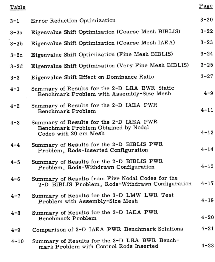
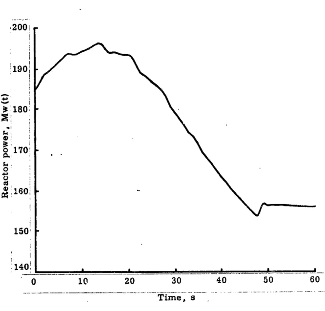
6-1 Total reactor power versus time for the 3-D LMW

problem, with. thermal-hydraulic feedback 6-24

6-2 Mean reactor power density versus time for the

full-core 3-D LRA BWR transient benchmark problem 6-39

A5-1 Normalized assembly power densities and errors for

the 2-D LRA BWR problem, "rods in"

configuration A5-1

A5-2 Normalized assembly power densities and errors for

the 2-D IAEA PWR problem A5-2

AS-3 Normalized assembly power densities and errors for the 2-D BIBLIS PWR problem, "rods in"

configuration A5-3

A5-4 Normalized assembly power densities and errors for the 2-D BIBLIS PWR problem, "rods out"

configuration A5-4

A5-5 Normalized assembly power densities and errors for

the 3-D LMW problem A5-5

A5-6 Normalized assembly power densities and errors for

the 3-D IAEA PWR problem (VENTURE reference) A5-6

A5-7 Normalized assembly power densities and errors for

Figure Page

A5-8 Normalized assembly power densities and errors for

the 3-D LRA BWR problem, "rods in" configuration A5-8

A5-9 Normalized assembly power densities and errors for

the 3-D LRA BWR problem, quarter-core, "rods

out" configuration A5-9

A5-10 Normalized assembly power densities and errors for

the 3-D LRA BWR problem, .full-core, "rods out"

configuration A5-10

A5-11 Normalized assembly power densities and errors for

the 2-D Zion 1 PWR problem A5-11

A6-1a Normalized assembly power densities for the 2-D

LRA BWR kinetics benchmark problem A6-2 A6-1b Temperature distributions for the 2-D LRA BWR

kinetics benchmark problem A6-9

A6-2a Normalized assembly power densities for the 3-D, quarter-core, LRA BWR kinetics benchmark

problem A6-12

A6-2b Normalized planar power densities for the 3-D, quarter-core, LRA BWR kinetics benchmark

problem A6-18

A6-2c Planar temperature distributions for the 3-D, quarter-core, LRA BWR kinetics benchmark

problem A6-24

A6-3a Normalized assembly power densities for the 3-D,

full-core, LRA BWR kinetics benchmark problem A6-27

A6-3b Normalized planar power densities for the 3-D,

full-core, LRA BWR kinetics benchmark problem A6-34 A6-3c Planar temperatures distributions for the 3-D,

LIST OF TABLES

Table v age

3-1 Error Reduction Optimization 3-20

3-2a Eigenvalue Shift Optimization (Coarse Mesh BIBLIS) 3-22 3-2b Eigenvalue Shift Optimization (Coarse Mesh IAEA) 3-23 3-2c Eigenvalue Shift Optimization (Fine Mesh BIBLIS) 3-24 3-2d Eigenvalue Shift Optimization (Very Fine Mesh BIBLIS) 3-25 3-3 Eigenvalue Shift Effect on Dominance Ratio 3-27 4-1 Summary of Results for the 2-D LRA BWR Static

Benchmark Problem with Assembly-Size Mesh 4-9 4-2 Summary of Results for the 2-D IAEA PWR

Benchmark Problem 4-11

4-3 Summary of Results for the 2-D IAEA PWR Benchmark Problem Obtained by Nodal

Codes with 20 cm Mesh 4-12

4-4 Summary of Results for the 2-D BIBLIS PWR

Problem, Rods-Inserted Configuration 4-14 4-5 Summary of Results for the 2-D BIBLIS PWR

Problem, Rods-Withdrawn Configuration 4-15 4-6 Summary of Results from Five Nodal Codes for the

2-D BIBLIS Problem, Rods-Withdrawn Configuration 4-17 4-7 Summary of Results for the 3-D LMW LWR Test

Problem with Assembly-Size Mesh 4-19

4-8 Summary of Results for the 3-D IAEA PWR

Benchmark Problem 4-20

4-9 Comparison of 3-D IAEA PWR Benchmark Solutions 4-21 4-10 Summary of Results for the 3-D LRA BWR

Table P age 4-11 Summary of Results for the Quarter-Core, 3-D LRA

BWR Benchmark Problem with Control Rods

Withdrawn 4-25

4-12 Summary of Results for the Full-Core, 3-D LRA BWR Benchmark Problem with Control Rods

Removed 4-26

4-13 Control Rod Reactivities in the 3-D LRA BWR

Benchmark Problem 4-28

4-14 Summary of Results for the One-Group IAEA

Benchmark Problem No. 2 4-31

4-15 Summary of Results for the 2-D Zion 1 PWR with

Explicit Core Baffle 4-36

6-1 Summary of Static Results for the TWIGL

Two-Dimensional Seed-Blanket Test Problem 6-3

6-2 Total Power Versus Time for the 2-D TWIGL Seed-Blanket Reactor Problem (Ramp

Perturbation): Sensitivity to Theta (f) 6-4

6-3 Total Power Versus Time for the '2-D TWIGL Seed-Blanket Reactor Problem (Ramp Perturbation):

Sensitivity to Number of Inner Iterations per Step 6-6 6-4 Total Power Versus Time for the 2-D TWIGL

Seed-Blanket Reactor Problem (Ramp Perturbation):

Sensitivity to Transient Convergence Criterion 6-7 6-5 Total Power Versus Time for the 2-D TWIGL

Seed-Blanket Reactor Problem (Ramp Perturbation):

Sensitivity to Time Step Size 6-8

6-6 Total Power Versus Time for the 2-D TWIGL Seed-Blanket Reactor Problem (Ramp Perturbation):

Sensitivity to Matrix Updating Frequency 6-9

6-7 Total Power Versus Time for the 2-D TWIGL Seed-Blanket Reactor Problem (Ramp Perturbation,

Fine Spatial Mesh) 6-10

6-8 Total Reactor Power Versus Time for 2-D TWIGL

Table P age 6-9 Execution Time Comparison for 2-D TWIGL

Seed-Blanket Reactor Problems (Coarse Mesh) 6-14

6-10 Power Versus Time for the 3-D LMW Test Problem

(QUANDRY) 6-16

6-11 Power Versus Time for the 3-D LMW Test Problem

with Control Rod Cusping Adjustment (QUANDRY) 6-18 6-12 Power Versus Time for the 3-D LMW Test Problem:

Comparison of Temporal Convergence of Transient

Solutions with Time Step Size = 500 ms 6-19 6-13 Power Versus Time for the 3-D LMW Test Problem:

Comparison of the Most Accurate Solutions for

Three Nodal Methods 6-21

6-14 Total Reactor Power Versus Time for the 3-D LMW

Problem with Thermal-Hydraulic Feedback 6-23 6-15 Summary of Results for the 2-D LRA Transient:

QUANDRY Calculations with Very Coarse Mesh 6-28 6-16 Summary of Results for 2-D LRA Transient:

QUANDRY Calculations with 1000 Time Steps,

Coarse Mesh 6-30

6-17 Summary of Results for 2-D LRA Transient: QUANDRY Calculations with 329 Time Steps,

Coarse Mesh 6-31

6-18 Comparisons of Nodal Solutions to the 2-D LRA

BWR Transient Problem 6-33

6-19 Summary of QUANDRY Results for the 3-D Quarter-Core LRA BWR Problem, Very Coarse Spatial

Mesh 6-35

6-20 Summary of QUANDRY Results for the 3-D Whole-Core LRA BWR Problem, Very Coarse Spatial

Chapter 1 INTRODUCTION

1. 1 OVERVIEW

An extensive knowledge of the spatial power distribution is required for the design and analysis of current-generation light water reactors. Efforts to answer safety questions which arise in conjunction with actual and hypothetical accident scenarios often require the knowledge of multi-dimensional transient power distributions. Accordingly, the nuclear reactor vendors and the nuclear utilities are under increasing pressure to develop techniques with which they can verify the safety of their reac-tors.

Several approaches to establishing that reactors are safely

designed come to mind. It is possible to build experimental facilities for each reactor design and to perform a multitude of static and

transi-ent experimtransi-ents designed to answer the pertintransi-ent safety questions. However, this option is frightfully expensive, of dubious value, and

practically impossible. Another alternative is to adopt ever more stringent operating limits and ultraconservative design techniques. This course of action leads to a poor utilization of resources, to a de-gradation of plant efficiencies, and ultimately to prohibitively expensive nuclear electrical energy.

A more promising means of answering the safety questions appears

to be the development of more sophisticated theoretical methods, which are capable of producing the required safety-related information. There are also economic incentives for pursuing this last course of action: It is possible that by increasing the accuracy of theoretical predictions and confidence in them, unnecessarily conservative design and operating margins may be relaxed.

Over the past two decades, finite difference methods have emerged as the standard computational technique used for calculation of the power distributions in nuclear reactors. Only in very recent years, since the development of the high speed digital computer, have finite difference techniques been capable of performing "relatively economic" three-dimensional calculations for light water reactors. To this date, three-dimensional transient calculations remain prohibitively expensive and a practical impossibility for use in "day-to-day" design and analysis of thermal reactors.

As a result, a large number of computational schemes have been proposed as alternatives to the computationally inefficient finite differ-ence techniques (1). In particular, certain nodal methods have reached high levels of sophistication and have been demonstrated to be orders of magnitude more computationally efficient than finite difference schemes (2). Some of these methods, however, are subject to company confidentiality. Therefore, the need to develop new methods for multi-dimensional transient reactor analysis still exists. The primary objec-tive of the author is to develop an efficient, economical, and accurate

method for the analysis of three-dimensional transient behavior of light water reactors.

1.2 SYNOPSIS OF THE PROBLEM

In most situations encountered in the analysis of light water reac-tors, it is sufficient to model the neutronic behavior of the reactor by a low order approximation to the formally exact neutron transport equa-tion. The most widely used of these approximations is multigroup

neutron diffusion theory. For this model, the set of time- and space-dependent coupled partial differential equations for which approximate

solutions are sought can be written as

V-D (rt)V09 (r,t) - E tg(r_, t)0 (r,t) + G

%(gg(rt)+(1-)xfg(rt))ckg,(rt)

ZX

G total number of neutron energy groups

Og = scalar neutron flux in group g (cm 2 sec) g

-3 Cd 2 density of delayed neutron precursors in family d (cm )

D 2 diffusion coefficient for group g (cm)

-1 E 2 macroscopic total cross section for group g (cm )

tg

E ,t9 macroscopic transfer cross section from group g' to

gg -1

group g (cm )

x prompt fission neutron spectrum to group g

V =mean number of neutrons emitted per fission

ly eigenvalue which makes all of the time derivatives identically zero

Ffg92macroscopic fission cross section for group g (cm) X 2 delayed neutron spectrum for family d in group g

Xd 2 decay constant for delayed neutron precursor family

d -1

d (sec )

d fractional yield of decayed neutron precursors in family d per fission

= total fractional yield of delayed neutron precursors D

per fission, _{( =}

₂₁

v = neutron velocity for group g (cm sec )

and the fission neutron spectrum is assumed to be that of the predomi-nant fissioning isotope. If the distribution of material properties in

space and time, the initial neutron flux distribution in space and energy, and the appropriate boundary conditions are specified, a unique solution to Eqs. 1-1 exists. The two most commonly used boundary conditions

applied to the outer surface of the reactor are, stated physically, that the neutron flux or the incoming neutron current for every energy group be identically zero. At any internal surfaces, continuity of neutron flux and the normal component of the neutron current are imposed for

every energy group.

The solution to Eqs. 1-1 is usually obtained by first assuming that the reactor is in a "critical" configuration. That is, all of the proper-ties of the reactor are independent of time and hence all of the time

derivatives in Eqs. 1-1 are identically zero. The static solution to Eqs. 1-1 is obtained by varying the parameter y (a critical eigenvalue)

such that a nontrivial solution to the static multigroup equations exists. The static multigroup equations can be written as

_V - D (r)V( (r)r g + ,(r)+XIV (r), (r) = 0;

g--g9- ~tg(39 g r)+ 9gg gy fg'-i

g'=1

g =1,2,...,G' (1-2)

In principle, the spatial power distribution in a reactor can be deter-mined by applying Eq. 1-2 and explicitly representing all of the geo-metrical detail which is present. The geometrical complexity of large current-generation light water reactors is so great that direct represen-tation of full geometrical heterogeneity is precluded for reasons of prac-ticality. The approach that is generally taken to alleviate this difficulty is to treat large spatial regions as homogenized. The actual spatial detail within each of the homogenized regions is treated in an auxiliary calculation, to obtain "equivalent homogenized diffusion theory

parameters" which are spatially constant within each region. The tech-niques used to perform this homogenization need not be limited to dif-fusion theory, and many such schemes have been devised over the years

(3). This homogenization is commonly performed for regions which contain one or several fuel assemblies in a radial plane (typically a rectangular region with sides of approximately 20 cm) and have an axial length of similar extent. The full core reactor calculation is thus re-duced to that of determining the spatial power distribution within a reactor containing several thousand homogenized regions. The author will not address the many problems associated with homogenization techniques, but rather, will approach the task of determining the spatial power distribution within a reactor which has been partitioned into

"homogenized" regions. The equivalent homogenized diffusion theory parameters for each region are assumed to be known.

1. 3 REVIEW OF -SOLUTION METHODS

Many methods for solving the static multigroup diffusion equations are presently available to the nuclear reactor community. Complete descriptions of each of these methods are much too lengthy to be included in this review. Only the comparative advantages and disadvantages of

several of the most widely used methods are summarized in this section. In finite difference schemes, low order difference approximations are used to represent the leakage term of Eq. 1-2, V- D (r) V4 (r). These finite difference methods possess several advantages over most

and the resulting algebraic equations are such that only adjacent nodes are coupled by the spatial leakage terms. One very important property of finite difference techniques is that they can be shown to converge to the exact solution of the multigroup diffusion equations in the limit of

infinitely fine mesh spacing (4). Also, as a consequence of the wide-spread use of finite difference methods, the associated numerical

methods have also reached high levels of sophistication. The only real disadvantage of finite difference schemes is that very fine spatial meshes are required to achieve acceptable accuracy (5). This problem is parti-cularly pronounced in regions near a water reflector in light water reac-tors, since the thermal neutron flux there is highly peaked. The need for fine mesh spacing translates into large numbers of unknowns, and hence, into excessive computational effort for multidimensional prob-lems. Nevertheless, finite difference techniques are reliable means of

generating solutions to the multigroup diffusion equations with which to compare the results of other methods, and despite their drawbacks for use with full core reactor calculations, they will probably continue to be the industry standard for quite some time to come.

In the past few years, many researchers have applied finite element techniques to solving the multigroup diffusion equations (6). In finite

element methods, the spatial shapes of the multigroup fluxes are repre-sented as polynomials over large homogeneous regions. Variational principles are generally used to determine the equations which specify the coefficients of the polynomials. It is possible to achieve a substan-tial reduction in the number of spasubstan-tial unknowns, for a given degree of

accuracy, over finite difference methods (7). The finite element

schemes also converge to the exact solution of the multigroup diffusion equations in the limit of infinitely fine mesh spacing. The major disad-vantage is that the coupling of the finite element equations is much more extensive than with the finite difference equations. Hence, it is gener-ally found that the reduction in the number of unknowns is offset by an increase in computational effort required to solve the resulting equa-tions (8). Since any reduction in computational effort over the finite difference techniques is at best marginal, finite element methods will probably not replace finite difference methods as an industry standard.

If it is imperative that the full spatial heterogeneity within a reactor be modeled, spatial flux synthesis schemes offer the largest reduction in the number of spatial unknowns. In synthesis schemes, precomputed expansion functions are obtained over large regions of the reactor, per-haps by two-dimensional (x-y) finite difference calculations with full geometrical detail. These expansion functions are combined by coef-ficients which are determined by solving spatial equations of a lower dimensionality, such as one-dimensional (z-dependent) equations. The equations for the unknown "mixing coefficients" are derived by applying a variational principle and demanding that the approximate solution obey the multigroup diffusion equations in a weighted integral sense. A major reduction in the number of unknowns is routinely obtained by many syn-thesis schemes, and the resulting equations are not difficult to solve (9). The unfortunate drawback of synthesis methods is that there is no sys-tematic procedure for choosing the expansion functions or the weighting

functions. Furthermore, rigorous error bounds on the synthesized solutions do not exist. This lack of error bounds has limited the wide-spread use of spatial flux synthesis. There are, however, many re-searchers who have used spatial flux synthesis with varying degrees of success (10).

Another class of techniques used to solve the multigroup diffusion equations are nodal methods. The quantities of interest in most nodal methods are the group-dependent neutron fluxes averaged over large spatial regions (nodes) and the neutron currents averaged over the faces of the nodes. No approximations to the formally exact neutron transport equation need to be made in the derivation of the nodal balance equations. The difficulty with the nodal methods is that relationships between the node-averaged fluxes and the face-averaged currents must be obtained. Many different schemes for determining these relationships have been proposed (11). Once the relationships between node-averaged fluxes and face-averaged currents are specified, equations with a structure similar to finite difference equations can be constructed. Thus, nodal methods possess much of the simple structure of finite difference

methods, while offering a substantial reduction in the number of un-knowns by utilizing node-averaged fluxes. Hence, if consistent, sys-tematic schemes for determining the flux-current spatial coupling can be developed, nodal methods appear to offer considerable promise as accurate, efficient techniques for solving the multidimensional neutron diffusion equations.

1. 4 MOTIVATION OF NODAL METHODS

Many researchers have recognized the potential accuracy and com-putational efficiency of consistently formulated nodal methods. Hence, many different schemes have been proposed to determine the flux-current coupling. Early nodal methods used crude approximations for the coup-ling terms and, consequently, had limited accuracy (12). Some attempts were made to circumvent the limited accuracy by imposition of ad hoc modifications ("refinements"'). These modifications increased accuracy, but they relied on trial and error adjustment of artificially introduced parameters to match higher order calculations. These methods were applicable only to a limited range of reactor conditions, and thus, were not widely accepted as viable design tools.

In recent years, however, systematic, consistent methods to deter-mine the flux-current coupling terms have been devloped by several researchers. Methods which use polynomial expansions of the fluxes and currents have produced extremely accurate solutions to the multi-group diffusion equations (13-15). An "Analytic Nodal Method" which employs analytic solutions of the one-dimensional, two-group diffusion equations to determine the spatial coupling has also been notably suc-cessful and has undergone several stages of refinement (16-18).

1. 5 OBJECTIVES AND SUMMARY

The objective of this paper is to extend the Analytic Nodal Method to three dimensions and to develop computationally efficient numerical methods for solving the time-dependent, multidimensional, 2-group

neutron diffusion equations. In Chapter 2, derivations of the static nodal diffusion equations and the Analytic Nodal Method are presented. Next, numerical techniques for solving the static nodal diffusion equa-tions are discussed (Chapter 3), and results of several static benchmark

problems are included (Chapter 4). The techniques employed to solve the time-dependent neutron diffusion equations are detailed in Chapter 5

and the solutions to a large number of two- and three-dimensional tran-sient problems are presented (Chapter 6). Finally, a summary of the investigation, conclusions about the Analytic Nodal Method, and recom-mendations for future research are given in Chapter 7.

Chapter 2

DERIVATION OF THE ANALYTIC NODAL METHOD FOR SOLVING THE STATIC MULTIGROUP DIFFUSION EQUATIONS

2. 1 INTRODUCTION

In a recent thesis, Cook demonstrated that many transients en-countered in light water reactor (LWR) safety analysis can be success-fully analyzed using assembly-sized thermal-hydraulic regions. (19). Cook also found that the LWR transient analysis code MEKIN (which uses a finite difference neutronic model) applied as much as 95 percent of its computational effort in certain problems to solving the neutronics equations (from which the average powers in the thermal-hydraulic regions were determined), and as little as 5 percent of the computa-tional effort was expended in solving the thermal-hydraulic equations. Therefore, a neutronic model which had averaged fluxes in the thermal-hydraulic regions as the only unknowns could be very efficient, and still provide the necessary information to model successfully most LWR transients.

Several years ago, Antonopoulos developed a method for solving the one- and two-dimensional diffusion equations which used exact difference equations (20). Although Antonopoulos solved these exact difference equations by approximation, Shober later introduced an exact method for solving the difference equations (16). This method, which was exact

in one dimension for any mesh spacing (provided the cross sections were spatially constant within each region) and had region-averaged fluxes as the only unknowns, would seem to be ideally suited for use in coupled neutronic thermal-hydraulic problems in which

assembly-sized thermal-hydraulic regions could be used.

In this chapter, the Analytic Nodal Method for solving the static multigroup diffusion equations will be derived, making use of Anton-opoulos' exact difference equations. In more than one dimension, exact solutions will be shown to exist only for very simple problems, and thus, an approximation will be required for more complicated (realistic) problems. Several approximations have been developed by other researchers and will be presented in this chapter for complete-ness. Throughout the derivation of the Analytic Nodal Method, it will be assumed that equivalent homogenized diffusion theory parameters, which are spatially constant over large regions, can be used. There-fore, only regions which have constant material properties will be con-sidered, and all derivations will be done in three-dimensional Cartesian geometry. It will be demonstrated that nodal diffusion equations can be derived, which have node-averaged fluxes as the primary unknowns and nearest neighbor spatial coupling in node-averaged fluxes.

2.2 DERIVATION OF THREE-DIMENSIONAL MULTIGROUP NODAL DIFFUSION EQUATIONS

The global reactor problem is treated in three-dimensional Carte-sian geometry, where x, y, and z represent the three coordinate direc-tions. A very general notation for the coordinate directions proves

quite useful; hence, u, v and w are used as generalized coordinate sub-scripts. The spatial domain is subdivided into a regular array of nucle-ary homogeneous right rectangular parallelepipeds (nodes) with grid indices defined by u2, vm, and wn where

i=1,2,...1 ; u,v,w = x

,M,n=

j

As an example of the future use of this generalized coordinate notation, the net currents on the faces of node (i,j,k) as a function of the two transverse directions are expressed as

Juij, k(vw)] = -[Di,

j,

a<I(u,

v u

This single equation actually expresses three equations: 1) The x-directed net current on the x xi face, as a

function of y and z (u = x, v = y, w a z)

2) The y-directed net current on the y y. face, as a

3 function of x and z (u = y, V= x,w z)

3) The z-directed net current on the z=zk face, as a

function of x and y (u = z, v = x, w = y) The node (i, j, k) is defined by

XE[zx,xi+1I

Y E[ y , yj+1I

The node widths are then defined as h = u +i I ; U = X,,z , and the node volume is

V. .a hihihk i,,k X y z

For convenience, the static multigroup diffusion equation, Eq. 1-2, is cast in conventional matrix form:

-V - [D(r)] V(0(r)] + [ET(r)] [#O(r)] ! [XI[vE(ri)T[

j(r)]

where

[r_)] is a column vector of length G containing neutron fluxes [D(r)] is a diagonal G X G matrix containing the diffusion

coefficients

[ET(r)] is a GX G'matrix containing the macroscopic total-minus-scattering cross section

[x] is a column vector of length G containing the fission neutron spectrum

[VE f(r)] is a column vector of length G containing nu, the mean number of neutrons emitted per fission, times the macroscopic fission cross section y is a critical eigenvalue of the global static reactor

problem,

The first step in the derivation of the nodal diffusion equations is to integrate Eq. 2-1 over the volume of an arbitrary node (ij,k) to obtain:

hi hk([j y z xi+1,

_jk

_jk+1'

_j1,k

+vi k _{j[ET ] [~i. .} ''3 k i,

j,

y i,j,k fiIjf kI i,jk where i,

j,1k

fj+1

Equation 2-2 is a rigorous statement of neutron balance for any node (I,

jk).

i,j,k [J

],

[is

the spatial flux distribution cannot be determined.

(2-2)

2. 3 DERIVATION OF SPATIAL COUPLING EQUATIONS

One method of obtaining a differential equation from which the spatial coupling of Eq. 2-2 can be determined is to treat the directions one at a time and spatially integrate Eq. 2-1 over the two directions transverse to the direction of interest, to obtain for direction u and node (,m,n), hmn vD+2 vm1 w n+1 2 -hm hw [D e, mjn]y u(u)]-[D mnJ m+ndvjf 1dw Iu .,Qm,n '' vm wn Ov X [O(u, v, w)] -[D 12 f M+1dv

J

= lhmhn[xI[vEf ]T[u (u)]; ux,y,z (2-3)

'Yv W _.e,m,n vUm~n vu w*uev where [0(1)f 1 vm+1 dv fwn+1 dw [0(u,v,w)]. uA,m,n hmhw vm wn

Equation 2-3, when multiplied by du, is simply a statement of neutron balance within a slab contained in node (2 ,m,n) which has the height and depth of the node, but which is of thickness du (in the u direction) about the point u. Hence, the two integrals represent the net rate at which neutrons leak out of the four surfaces of the slab which are transverse

to direction u. The following notation for the net leakages is convenient: n vwn 2 hnw[L v (u)]-Djp ₁ ,m,n ] j m+1 dv f +1 dw 20(u~vw); w mmn vm w n (2-4) U = ,yoZ V =XyZ W = x,yZ; v #u w *u #v.

Equation 2-4 possesses the property that when integrated over [uAui+ll and divided by h1 it yields

U 4f'+1 _{du [L} u _A.0,m,n (l .9+1,m,n m n

.J

which is the nodal face-averaged, v-directed, net leakage. By defining a sum of the two net leakages transverse to direction u, per unit u, divided by hmhn as v w [S (u)]--[L()]+ ul,m,n hm vilmn v 1 _L (u)] hn w w u =x,y,z v*u w u0v,

Equation 2-3 can be cast in the form

(2-6) ;

-[DA mnl [ (u)]F+,([ET I -4[X][vsf 1

' ' 8u 1m,n A,m,n AMn

X [4 n (u)] = - [Sue,m,n(u)]); u= x,y,z. (2-7)

To obtain relationships between the node-averaged fluxes and the face-averaged net leakages, one need only solve Eq. 2-7 for [ n(u)J and integrate this "one-dimensional" flux over the node. Unfortunately, the u-dependence of the transverse leakage source term on the right-hand side of Eq. 2-7 must be known or approximated if the solution of the equation is to be found. This circumstance makes necessary the first, and only, approximation of the Analytic Noda Method.

2. 3. 1 The "Buckling" Approximation

The possibilities for the approximation of the transverse leakage shape in Eq. 2-7 appear to be unlimited. It does, however, seem reasonable to expect that the more complicated the assumed shape, the more difficult it will be to solve for the one-dimensional flux.

For this reason, Shober (16) initially assumed that the transverse leakages and the one-dimensional fluxes had the same shape. That is, the transverse leakages were assumed to obey the equation

. [B u e,m~n uf n(u)] = [Su n(u)] ; u= x,y,z. (2-8) The values of the diagonal matrix [Bu ] were assumed to be inde-pendent of u within node (1,m,n) and were found by integrating Eq. 2-8 over [u..,u1+11 and dividing by h to obtain

(B I[f ]-e ]=[LI+-1-L I

Bu Amn h A,m,n hnw _,M,n

[; u=w,y,z. (2-9)

This "buckling" approximation would be exact if the fluxes were spati-ally separable -within node (i,

j,

un-u ,mn

known. Hence, Eq. 2-7 could be easily solved for OUf ,m,n(u)], which in turn could be integrated to obtain the desired relationships between

[-uimn'' I-1,m,n1 , ReTm,n'' and [T+1 ,M,n'*

However, Shober found that use of the buckling approximation led to large errors in highly nonseparable problems.

2. 3. 2 "Flat" Approximation

As an alternative to the buckling approximation, Shober (16) then approximated the transverse leakage shape as spatially flat across each node, that is,

[S m (u)]=[Fu I; u=x,y,z. (2-10)

Shober demonstrated the superiority of the "flat" approximation over the buckling approximation for several highly nonseparable problems. He has also implemented a "two-step" transverse leakage approximation in which the leakages were assumed to consist of two piecewise constant segments within each node (17). Results from Shober's work indicated

that, as expected, the two-step approximation was substantially more accurate than the flat leakage approximation.

Despite Shober's encouraging results with the two-step Analytic Nodal Method, other researchers had found that more accurate results could be obtained by expanding the transverse leakages in higher order polynomials (13-15). This led Greenman, by suggestion of Finneman (21), to incorporate a quadratic approximation for the shape of the transverse leakages into the Analytic Nodal Method (18).

2. 3. 3 Quadratic Approximation

The quadratic polynomials suggested by Finneman were chosen in such a way as to uniquely determine the shape of the transverse leakage in a node by utilizing the average transverse leakages in three adjacent nodes. This approximation leads to a functional form of the net leakage transverse to direction u given by

[Su (u)J Wu ]P (u) +

[U

m,n A-1,m,n A uA,m,n A

+ [u

JP

uA+lmn , u1

.9

where each of the p's is a quadratic polynomial in u. The constraints imposed on the expansion functions, stated physically, were that the integral of the transverse leakage approximation over each of the three adjacent nodes preserve the average transverse leakage of that node. In mathematical terms, these conditions imply the following constraints:

1 fLu, f+A'+1 du p +e(u) = 6_A'A"l;

_u

x,y,z (2-12)

u+' '=0-1,O,1

.Q" =-l,0,1 _,

where 6 , is the Kronecker delta defined by

6 1

ef

l

The expansion functions of Eq. 2-12 are uniquely determined by the mesh spacing in direction u. It is important to note that the expansion for node (.Qm,n) is used only for that node, despite the fact that the expansion also preserves the average transverse leakages in nodes (A-1,m,n) and (1+1,m,n). This form of the transverse leakage is par-ticularly useful since it involves only average transverse leakages which are already unknowns in the nodal balance equation, Eq. 2-2. However, although this transverse leakage expansion is unique, there is no a priori reason to believe that it is the "best" quadratic approximation to the transverse leakage within node (A,m,n), for which it is used. This point will be discussed in detail in Chapter 4 after specific examples have been introduced. A complete derivation of the transverse leakage expansion functions for nonuniform mesh spacing is given in Appendix 1.

2.4 METHOD FOR SOLVING THE SPATIAL COUPLING EQUATIONS WITH QUADRATIC TRANSVERSE LEAKAGE

In principle, solving the spatial coupling equation to obtain relation-ships between node-averaged fluxes and face-averaged net leakages is quite simple. In the Analytic Nodal Method, the spatial coupling equation,

[D I,ml,n' 8 2[(o T 2u (u)] + ( Ou .,m,n X

[US

is solved analytically. The transverse leakage expansion of Eq. 2-11 can be expressed in an alternate, but entirely equivalent form, as

(U)I+v.[-g

AA+1,

2

2-I - - _('U _-_u

(u)=au + bu-(Ut) + - u-UQ

2 2 2 h ~-2 hU

2

Pu+1(u)=au + bu\2/ + cu 2)h ; u x,y, z

u u

Hence, Eq. 2-14 can be rewritten as

+ ( [fu_S+lm,n x-( _m, + (['u Ul+1, M, n U-1,m,n (2-15)

us-1lm n

u2,rn)

);

Substitution of the approximate form of the transverse leakage given by Eq. 2-16 allows Eq. 2-7 to be expressed in P1 form as

j[Qui

[St

I U9 0m-, nn *.9 s m .n .9U,m,n

u = X,y,Z

where

u ,mnA(t.9)]= ColAum JUY(te) n(te)], I

(2. 17)

[D

Mnl

[0]j

[0]

LIST_{A, m, n}

[S' ~(t )

=

101,2(-[$]-[

[S

_I

UAM,n(u

tAU-U ,

and the transverse leakage has been split into three pieces, a "flat," a "linear," and a "quadratic" defined by

1Sf1 ]sR ]+([ -[)a'

A

I,M,n

U -1,m,n

F A9,

n UA

.A

I

[Sq } = (([ ~I - [s I) c~

u Pmun-1,mn U, m, n U.

+](u+-,su n])ct ); u=x,y,z. (2-18)

lsue~~m~ IM,n A

The procedure for solving Eq. 2-17 for the relationships between face-averaged net leakages and node-face-averaged fluxes is now conceptually straightforward. For each node, and each direction u, the following seven steps are taken:

1) Three particular solutions to Eq. 2-17, on the interval 0<t <huI are determined for the flat, linear, and quadratic transverse leakage source terms, subject to the boundary condition

[Qp(t1=0)] = 0 .

2) The homogeneous solution to Eq. 2-17, on the interval 0O<t <h us is obtained subject to the boundary condition

[ozh(t1=0)] = [.Nup]

3) The particular and homogeneous solutions to Eq. 2-17 from Steps 1 and 2 are combined to obtain an analytic expression for [(t₂)] on the interval 0 < t <h.

4) The analytic solution of Step 3 is integrated over the interval [0,h] and a relationship between node-averaged*fluxes and face-averaged net currents is obtained in terms of[WU). 5) Steps 1-4 are repeated for the interval 0< <hu 'but

[cp(t _ =hu1 )] = 0 [h(t _{1_1u)] = [O(u )}

to obtain another equation relating node-averaged fluxes and face-averaged net currents in terms of [O(u )].

6) Since both solutions in Steps 4 and 5 are expressed in terms of [U(u)], the two equations are used to eliminate

[um n(uA)], as this surface flux is not an unknown in the nodal balance equation, Eq. 2-2. Thus, it is possible to find a relationship between node-averaged fluxes, face-averaged net leakages, and [J a ,M,n(uY)] 1 .

7) Steps 1-6 can be repeated to derive a relationship between node-averaged fluxes, face-averaged net leakages, and

[Ju+m (u1+1)] Taking the difference of these last two I9+1,m,,n

relationships finally allows one to obtain an equation relating node-averaged fluxes and face-averaged net leakages.

The actual application of the aforementioned procedure is quite long and tedious; it is presented in Appendix 2.

The final equations relating node-averaged fluxes and face-averaged net leakages can be expressed in the form

[Lu _{, M,nl} 1f-2 ,m, n ]uw[ ] = [F ][j ]+ [F ]I U1Mn9-1, mo _u

_n

I

Equation 2-19 reveals that the u-directed net leakage is coupled to node-averaged fluxes in three adjacent nodes in the u-direction, as well as to the transverse leakages in five adjacent nodes. The global reactor

prob-lem is much easier to visualize if Eq. 2-2 and Eq. 2-19 are cast in super-matrix form with the following definitions:

[4'] =a column vector of length G*I*J*K (s N) containing the node-averaged fluxes (ordered first by group, then x-direction, then y-x-direction, and finally z-directiop). FU] a column vector of length N containing the u-direction

net leakage

[Ful e a block tridiagonal matrix of order N X N containing the elements of [FtR _I

1 ,m,n

[GU]

=

1,m,

n

*, a block diagonal matrix of order N X N containing the elements of V.i.k[ET

i,3,k Tpj,k

[M = a block diagonal matrix of order N X N containing the elements of V ,&j k[x][V Ef

The resulting super-matrix equation can be written as

[F ]

-

[I]

[M]

[0]

[0]

[0]

hihk[I] _{hihi [I]} x z x y A-[G ] hU[G] y z

-[I]

_hk[Gy]

[0]

[0]

[0]

[01

[o

1

[0]

[o]

[01

[01

[0]

[0]

The global reactor equation as expressed in Eq. 2-20 is of the form of a classical eigenvalue problem,

[AfIm'[B] [X]

except for the fact that the elements of [Al depend on the eigenvalue 7. Equations 2-2 and.2-19 form the basis of the Analytic Nodal Method with a quadratic transverse leakage approximation. These equations,

along with the appropriate boundary conditions applied to the reactor

[F1

[L])

[Lyz

[U]

[L])

surface (Appendix 2), fully specify the global system of static nodal diffusion equations.

2. 5 SUMMARY

In this chapter, and its related appendices, a complete set of nodal diffusion equations have been derived from multigroup diffusion theory. The only approximation that was found to be necessary (in addition to the original assumption of homogenized nodes) was that the spatial shape of the transverse leakage within a node could be fit to a specific quad-ratic polynomial. The resulting equations were written in terms of node-averaged fluxes and face-averaged net leakages. Nearest neigh-bor spatial coupling was obtained in node-averaged fluxes, but not in face-averaged net leakages.

In Chapter 3, the numerical methods used to solve the nodal dif-fusion equations will be discussed. In addition, the numerical proper-ties of the equations will be examined and the consistency of the Analytic Nodal Method will be demonstrated. Applications of this nodal method to several two- and three-dimensional benchmark problema are pre-sented in Chapter 4.

Chapter 3

NUMERICAL CONSIDERATIONS

3.1 INTRODUCTION

In Chapter 2, the spatially-discretized static nodal diffusion equa-tions were derived for the solution of the multigroup diffusion equaequa-tions. A method of determining the spatial coupling coefficients, subject only to the assumption that the transverse leakages could be fit by a

quad-ratic polynomial, was derived for the two-group case in Appendix 2. In this chapter, the numerical techniques used to solve the two-group

analytic nodal diffusion equations are' presented. The consistency of the Analytic Nodal Method is also demonstrated for the case of infinitely fine mesh spacing. Results of optimizing several of the schemes used to accelerate the convergence rate of the iterative process are also

presented. The solutions to many static reactor configurations are contained in Chapter 4.

3.2 NUMERICAL PROPERTIES OF THE ANALYTIC NODAL DIFFUSION EQUATIONS

The equation for which a solution is sought in the Analytic Nodal Method is given in Chapter 2, by Eq. 2-20. This super-matrix equa-tion is a set of linear equaequa-tions in the four vector unknowns,

[7],

coupling in the node-averaged flux terms and most of the coupling in the face-averaged net leakage terms. It is known from physical prin-ciples that the net leakages will be small compared to the average fluxes in a large number of reactor configurations. Therefore, Eq.

2-20 has the undesirable characteristic that the spatial coupling is dominated by the net leakage equations. This situation is altered by substituting the last three blocks of equations into the first block of equations to obtain

[H(v]

[r][@

,

x

[G

_]1

A1

[G1

z

)

[M]

10]

f0]

0]

[0

[o]~

[o]

[o]

[o]

[P>

[]

= col{[I], [Lxi, [LJy1,

[L}

.

Since each of the matrices [Ful is block (2 X 2) tridiagonal, Eq. 3-1 has substantially more spatial coupling in node-averaged flux terms than does Eq. 2-20. Equation 3-1 is clearly an eigenvalue problem in which the elements of the matrix [H] depend on the eigenvalue.

Any iterative scheme that is used to solve Eq. 3-1 will require that the matrices [H] and [P] have certain properties in order to guar-antee successful convergence. Therefore, it is very useful to examine the properties of the matrices in Eq. 3-1.

The matrix [P] is quite simple. The only non-zero submatrix of the matrix [P] is [MI, and the matrix [M] is block diagonal with non-negative components (all fission cross sections are nonnon-negative).

Unfor-tunately, the matrix [H] is not nearly as simple. In the general'case, the only property of the matrix [H] that can be guaranteed is that all of its components are real.

There is, however, at least one case in which the properties of the matrix [H] can be specified. This special case is in the limit of infi-nitely fine mesh spacing. As the mesh spacings, hI, go to zero, the basic spatial coupling matrices, as defined in Appendix 3, become

1/D 0 ~h

Autm,n

B u1

0 uIsm - i 0

.-r

1/D

[+

Us[Da

[n

()8

With these spatial coupling matrices, the flux coupling coefficients, as defined in Eq. A2-14, in the limit of infinitely fine mesh spacing become

- [Ft'] =

[tmn

1=n

r

r

01

2+I,

@uJ

Thus, all of the matrices, [FuI, in Eq. 3-1 are block tridiagonal and diagonally dominant with components that are all of order 1/h. By ex-amining the leakage coupling matrices of Eq. A2-14, one finds that all of the matrices, [Gu] in Eq. 3-1 are of order h. Therefore, the first block of equations in Eq. 3-1 has coefficient matrices with terms of order h (flux terms) and terms of order h2 (leakage terms). Hence, in the limit of infinitely fine mesh spacing, the order h2 terms can be neglected and Eq. 3-1 becomes

[F][] = 1

[M][1

The net leakages of Eq. 3-1 do not enter directly into the nodal diffu-sion equations in the limit of infinitely fine mesh spacing. Close ex-amination of the flux coupling matrices of Eq. 3-3 reveals that Eq. 3-4

is actually a finite difference approximation to the two-group diffusion (3-3)

equations. The actual form of these difference equations is not that of the conventional finite difference equations with fluxes evaluated at the corner points of homogeneous volumes, but rather is that of a less fre-quently used formulation of finite differences with fluxes evaluated at the centers of the homogeneous volumes. Nevertheless, an important consequence of this reduction to the finite difference equations in the limit of infinitely fine mesh spacing is that the Analytic Nodal Method is guaranteed to converge to the exact solution of the two-group diffu-sion equations in this limit (23).

As a result of the elimination of net leakages in Eq. 3-1, the pro-perties of matrices [F] and [M suffice to determine completely the characteristics needed to guarantee convergence of the Analytic Nodal Method. Examination of Eq. 3-3 reveals that the matrices, [Fu] are

1. Real

2. Irreducible 3. Symmetric

4. Diagonally dominant.

From these properties, it can be proved that Eq. 3-4 has the following properties (23):

1. There exists a unique positive real eigenvalue, Ty, which is greater in modulus than all other eigenvalues. 2. The eigenvector corresponding to the eigenvalue 'Ti

is unique and positive.

3. 3 to demonstrate that the numerical schemes chosen to solve the Analytic Nodal Diffusion equations can be guaranteed to work in the limit of infinitely fine niesh spacing.

3.3 ITERATIVE STRATEGY FOR SOLVING THE STATIC NODAL DIFFUSION EQUATIONS

This section details the iterative strategy used to solve the static nodal diffusion equations, Eq. 3-1. Frequent use will be made of the properties of the matrices in Eq. 3-1, for the case of infinitely fine

mesh spacing, despite the fact that these properties cannot be shown to exist (and perhaps do not exist) in the general case.

3. 3. 1 The General Iterative Scheme

The general scheme for solving Eq. 3-1 is as follows: 1. An initial guess for -y (usually -y= 1.0) is used to

evaluate the components of the mptrix [H]. 2. An accelerated fission source (outer) iteration

is employed to determine iteratively the maxi-mum eigenvalue and corresponding eigenvector (y and [01 ).

3. After several outer iterations (usually 5-10), the latest estimate of 7 is used to update the components of the matrix [H].