Arbitrage with holding costs : a utility-based approach

HD28

•M414

no.

9/

WORKING

PAPER

ALFRED

P.

SLOAN

SCHOOL

OF

MANAGEMENT

ARBITRAGE

WITH

HOLDING

COSTS:

A UTILITY-BASED

APPROACH

by

Bruce

Tuckman

and

Jean-Luc

Vila

Latest

Revision:

December

1991

Working

Paper

No.

3364-91-EFA

MASSACHUSETTS

INSTITUTE

OF

TECHNOLOGY

50

MEMORIAL

DRIVE

ARBITRAGE

WITH

HOLDING

COSTS:

A

UTILITY-BASED

APPROACH

by

Bruce

Tuckman

and

Jean-Luc

Vila

Latest

Revision:

December

1991

M

l.T.

LIBRARIES

1

1M*

Arbitrage

With

Holding

Costs:

A

Utility-Based

Approach

by

Bruce

Tuckman

Stern

School

of Business,

New

York

University

and

Jean-Luc

Vila

Sloan School of

Management,

M.I.T.

This version:

December,

1991

We

would

like to thank participants in the

N.Y.U. and

Cornell

Finance Seminar

Series,

participants in the 1990

AFA

and

AFFI

meetings,

and

an

anonymous

referee for helpful

comments

and

suggestions.

Abstract

Unit

time costs, or holding costs, are incurred in

many

arbitrage contexts.

Well

known

examples

include losing the use of short sale

proceeds

and

lending funds at

below market

rates in

reverse repurchase agreements. This

paper

analyzes the investment

problem

of a risk averse

arbitrageur

who

faces holding costs.

The

proposed

model

allows prices to deviate

from

their

"fundamental" values without allowing for riskJess arbitrage opportunities. After characterizing an

arbitrageur's optimalstrategy, the

model

is

examined

in thecontextofthe

Treasury

bond

market.

The

analysis reveals that holding costs are an important friction in this

market and

that they

can

be

Arbitrage

With

Holding

Costs:

A

Utility-Based

Approach

Financial

economists

have

made

great use of the notion of arbitrage in frictionless markets.

Researchers

define arbitrage as a set oftransactions

which

costs nothing

and

yet riskJessly provides

positive cash flows.

They

then

assume

that arbitrage opportunities

never

exist

and

derive precise

implications

about

the relative prices of traded securities.

The

presence

of

market

frictionscomplicates thestory. In the simplestof models, trading costs

make

it impossible to riskJessly exploit small price deviations

from

arbitrage-free relationships.

Therefore,

when

market

prices

do

not admit riskless arbitrage opportunities, arbitrageurs

do

nothing.

When

market

prices

do

admit

such

opportunities, arbitrageurs bet all they

have

on

the sure

proposition that prices will

be back

in line at the maturity date of the underlying securities.

While

this simple

model

can explain the empirical regularity of price deviations

from

"fundamental value,"1

more

careful portrayalsof

market

frictions

make

for richer

models

ofarbitrage

activity.

Brennan

and Schwartz

(1990), forexample,

show

that trading costs

and

position limits in the

stock index futures

market

can

make

it valuable to close a position before maturity.

As

a result, it

may

be

worthwhile

to

open

a position

even

when

the costs of

opening

it plus the costs ofclosing it

at maturity

exceed

the price deviation

from

fundamental

value. This

paper

contributes to the theory

of arbitrage pricingwith

market

frictions in

two

ways. First, it focuses

on

a

somewhat

ignored aspect

of true-to-life arbitrage activity,

namely

unit time costs, or holding costs.

Second,

it builds a

model

which

rules out riskless arbitrage opportunities without

removing

all incentives to exploit

market

mispricings.

As

a result, risk averse arbitrageurs

do

not sit idly by or bet all the have.

They

take a

finite, risky position if the mispricing is large

enough

and

adjust its size as the mispricing changes.

This behavior is consistent with the casual empirical observation that professional arbitrageurs

Thephrase "fundamentalvalue'is10 mean the arbitrage-tree pricewhen there areno market frictions. Innosense dowe mean

2

routinely find

and

take

advantage

ofdeviations

from fundamental

values.

Section I describes

how

holding costs

can

transform riskless arbitrage opportunities into

potentially profitable but risky investment projects. It

then

argues that holding costs are important

in

many

different arbitrage contexts.

Section II presentsa

model

ofarbitrageactivity.

The

scene

issetwithaholdingcost structure

and

an

exogenous

mispricing process that, in combination,

do

not

admit

riskless arbitrage

opportunities.

The

paper

then derives the partial differential equation governing a risk averse

arbitrageur's optimal,

dynamic

strategy.

For

the case of negative exponential utility it is

shown

that

1) arbitrageurswill hold a position if

and

only if the potential gains are large

enough,

2) the position

isfinite,

and

3) arbitrageurswilltake a position

even

with

an

instantaneouslynegative

expected

return

since

any

future losses will

be

accompanied

by greater arbitrage opportunities.

Section III

examines

the model's assumptions in the context of the U.S.

Treasury

bond

market, estimatesthe

parameters

ofthemodel,

and

numericallysolvesthepartialdifferentialequation

ofsection II using those parameters.

The

data support the contention that holding costs are quite

important, relative to trading costs, in preventing riskless arbitrage.

The

data also support the

assumption

ofan autoregressive processfor the deviationof prices

from fundamental

value. Finally,

the numerical solutions reveal an "option effect"

and

a "risk effect" in the determination ofposition

size

and

allow for

an

assessment of the relative

importance

ofthe

two

effects.

Section

IV

concludes

and

discusses

avenues

for future research. In particular, this

work

can

be

viewed

as a first step towards building an equilibrium

model

ofarbitrage activity in the presence

of holding costs.

Such

a

model

holds the

promise

of being able to provide tighter price

bounds

3

I.

Holding Costs

and

Risky

Arbitrage

Consider

two

portfolios,

A

and

B,

which

provide identical cash flows

over

time and, at the

time of the last cash flow,

must have

identical

market

prices. Nevertheless, for

some

reason, the

market

prices ofthe portfolios,

P

A

and

P

B, differ by an

amount

x.

Assuming

that

P

A

_>

P

B, investors

in frictionless

markets

will short portfolio

A

and purchase

portfolio B, realizing x today

and

incurring

no

future cash inflows oroutflows.

Although

this

paper

could

have

assumed

that institutions

were

such

as to allow the arbitrage

just described, the

model

to be presented in section II builds

on

a

more

realistic description ofshort

sale agreements. In order to short portfolio A, an investor

must

borrow

the securities

from

somewhere.

Furthermore,

the lender of the securities will require collateral in order to

ensure

the

eventual return ofhis securities. Therefore, the arbitrage

must be

arrangedas follows: lend

P

A

dollars

to the holder ofthesecurities (or, equivalently. post

an

interest-bearing security

worth

P

A

), take the

securities in

A

as collateral, sell these securities for

P

A

,

borrow P

B

,

and purchase

portfolio B. In this

more

realisticsetting, the investor neitherpays nor receives

any

money when

establishing his position,

but realizes the future value ofx

upon

closing the position.

In frictionless markets, investors

would

wish to arbitrage

ad

infinitum, leading to the

conclusion that, in equilibrium,x

must

equal 0. Introducing holding costs

changes

arbitrage behavior

in

two

important ways. First, the no-riskless arbitragecondition only requires that x

be

no

larger than

the present value of the

accumulated

holding costs,

from

the

opening

of the position to the time

when

the

two

portfolio prices

must

be equal.

Second,

for smallerx, investors face a risky investment

opportunity: ifx falls to quickly

enough,

then the costs ofeffecting the arbitrage will

be

small

and

the transaction will

have proved

profitable. If,

on

the other hand, x

does

not fall quickly

enough,

the

accumulated

costs will

wipe

out the realized gains.

4

commodity

willusually incur unit time costssince investors

must

oftensacrifice theuse ofatleast part

of the short sale proceeds.2 In the case of stocks, it is true that institutions with large client bases

can take short positions almostcostlessly. Nevertheless, smaller firms

engaged

in arbitrage activity

do

incur holding costs

when

short-selling stocks.3

Second,

trading in futures

markets

may

generate

holding costs since at least part of

margin

deposits

may

not earn interest.4 Third,

banks

making

markets

in forward contracts often charge a per

annum

rate over the life of the contract.5 Fourth,

deviations

from

desired investment strategies

caused

by having to

meet

collateral requirements can

be

thought

of as unit time costs.6

The

model

ofthis

paper

focuses

on

holding costs

and

ignores trading costs for a

number

of

reasons. First, despite their ubiquitousness, holding costs

have

not received

much

scholarly attention.

Second, trading costs

would

obscure the qualitative nature of this paper's results.

Trading

costs

transformstrategies

which

continuouslyadjustholdingsinto strategies

which

discretelyadjustholdings,

where

the frequency of adjustment decreases in the trading costs. Since this effect has

been

studied

elsewhere,7 there is little

danger

that focusing

on

holding costs will

prove

misleading. Third, while

the trading costs ofprofessional traders

and

arbitrageurs

can be

extremelysmall, the

above examples

and

the discussion to follow reveal that their holding costs

need

not

be

trivial.

One

ofthe easiest contextsin

which

toestablish

both

the

importance

ofholding costs relative

to trading costs

and

the absolute

magnitude

of holding costs is the

Treasury

bond

market.

The

major

" _{Forthe case of stocks,see. forexample.Cox}

and Rubinstein (1985), pp. 98-103.

We

wouldliketo thankBillyRaoofSusquehanna InvestmentGroupforthiscomment.

4

See.for example.Duffie (1989). pp. 58-68.

5

See.for example.Anderson(1987), p. 198.

6

_We

would liketothankPeterCarrforthissuggestion.

See. for example.Dumasand Luciano (1990). Hodgesand Neuberger (1989), and Fleming.Grossman. Vila, and Zanphopoulou

5

trading costs in this market,

namely

bid-ask spreads

and brokerage

fees, are typically small, totalling

about

3/32 of

one

percent

and

1/128 of

one

percent, respectively.8

The

major

holding costs in the

government

bond

market

are reverse spreads. Recall that

bonds

are sold short

through

reverse

repurchase

agreements

in

which

the short sellerlends

money

and

takes thesecurity

he wants

toshort

as collateral.

The

reverse spread is defined as the difference

between

the lending rate

on

general

collateral

and

the lending rate

on

specific collateral. In other words, the reverse spread is the rate

available

when

any Treasury

bond

willserve ascollateral

minus

the rate available

when

onlya specific

Treasury

bond

will serve as collateral. This spread is usually positive9

because

the difficulties in

finding the

owner

ofa particular

bond

and

the likelyattempts of other

would-be

shorters to find the

same bond

translates into an opportunity loss

on

the

money

lent

through

reverses.

Stigum

(1983)

reports average spreads of

.25%

to .65%.10

Now,

to

compare

the

magnitudes

of trading costs

and

holding costs, consider shorting

$100

face value of a par

bond

and

maintaining the position until

maturity.

The

trading costs

come

to

about

10 cents and, with a spread of .5%, the holding costs

exceed

the trading costs for maturities longer than

about

2 1/2

months.

The

price data presented in

section III

show

that, for all but the shortest maturities, holding costs

do

more

than trading costs to

inhibit riskless arbitrage activity.

Two

recent empirical papers serve as excellent motivations for the present analysis. Cornell

and Shapiro

(1989)

document

both

the persistent mispricing of a particular

Treasury

bond

and

the

attempts ofarbitrageurs, facing holdingcosts, to profit

from

thatmispricing.

Amihud

and

Mendelson

(1990), studying the effects of liquidity by

comparing

the prices of

matched-maturity

Treasury bills

and

notes, find that notes are

cheap

relative to bills

and proceed

to

examine whether

these price

8

See Stigum(1990). pp.649-650 and p.669.

9

See Stigum(1990). pp. 596-597.

10

6

differences can

be

exploited. Considering only trading costs, as captured by the bid-ask spread

and

brokerage

costs, riskless arbitrage opportunities

seem

rampant.

Adding

holding costs,

however, most

of these

money

machines break down.

11

Another

motivationforthe analysis of holdingcosts

stems

from

therelativelyrecentliterature

about the source of

market

mispricings.

Some

authors (e.g.

De

Long

et al. (1990)

and

Lee

et al.

(1991))

have

hypothesized that investors' short

term

horizons allow for persistent deviations

from

fundamental

values. This

paper

reveals that holding costs, in effect, generate myopia.

Even

though

arbitrageurs

have an

investment horizon equal to the maturity of the underlying securities, holding

costs discourage the

maintenance

of long-term arbitrage positions. Therefore, holding costs

may

be

viewed

as a particular

way

to

endogenize

investor impatience.

II.

The Model

This section

models

the behavior of risk averse arbitrageurs

who

incur holding costs

and

observe prices that deviate

from

fundamental

value.

To

allow for the possibility of arbitrage

opportunities, begin by

assuming

that thereexist

two

portfolios.

A

and

B,

which

are characterizedby

identical cash flows

through

their

common

maturitydate, T.i: Let their date-t prices

be

P*

and

P^,

respectively.

Let x,

=

P*-P^

denote

the difference

between

the prices of these portfolios

on

date t.

While

it

would

be

ideal to

endogenize

the stochastic process governing theevolution ofx

t,

this

paper

follows

The authors actuallyconsiderthe bid-ask spread and then add both brokerage costs and holdingcosts. Nevertheless, because

brokeragecosts are so small in thismarket, the resultstated in thetext holds aswell.

While thisassumptionseemsinnocuous enough, it doesruleout concurrent investmentsin othernskyassets.This simplification

allows the model to abstract from the portfolio effects which would arise from holding othernsky assets in addition to an arbitrage

7

others13 in talcing the process as

exogenous

in order to focus

on

the investment

problem

facing

arbitrageurs.

The

assumed

evolution ofx, should exhibit the following properties:

1) x

_T

=

0, i.e. the price deviation disappears at maturity.

2) x, is

never

so large as to admit riskless arbitrage opportunities.

3) x, tends towards zero.

4)

The

larger the absolute value ofx,, the fasterx

t tends

toward

zero.

The

last

two

properties attempt to infuse the process with an equilibrium flavor. Property 3)

captures the idea that deviations are transient. Property 4) reflects the notion that larger deviations

will

be

exploited

more

readily, and. as a result, tend to vanish at a faster rate than smallerdeviations.

In order to find a process

which

satisfies (1)

and

(2). begin by

determining

the permissible

range ofx

t

.

Along

the lines of the motivations discussed insection I. let

c>0

be

the holding cost per

unit time per portfolio unit.14 Also, let r

denote

the arbitrageur's cost of capital.

Then,

the present

value cost of maintaining a unit short position

from

date t until maturity is

T

J"

ce-

r(s-l)

ds . t

Letting t

=

T-t. the time to maturity,

and

denoting this cost function by s(t),

s(t)=

_f

(l-e"") (1)

If the absolute value ofx exceeds s(t) at any time, then a riskless profit could

be

made

through the

arbitrage described at the start of the previous section. Therefore, to guarantee that |x,|

<

s(t).

generate the process x, in the following way:

See. forexample.Brennanand Schwartz(1990). Recently.Holden (1990) has endogenizedamispncing process byassumingthai aclientele effect splits themarket and that eachsegment is periodically hit by liquidityshocks.

14

Inthe context of the U.S.Treasury market,the holding costcanchangeasthe arbitrageursrolloverexpiringrepurchase agreemenis Itseems best,however, to postpone modellingc until it isendogenized to reflect the collectiveactivityof arbitrageurs. Furthermore, in

ordertomodelthe nskless arbitrageboundaryinasimpleway.ithas furtherbeen assumedthat theholding cost isper portfoliounit. In

8

x,

=

s(t)4>(z,) (2)

where

z, is

an

underlying state variable

and

<J> is a function

from

(-°o,

+

«>) to (-1,1)

which

preserves

the sign of z

and

increases in z. Notice that this setup also ensures that x

_T

=

since s(0)

=

0.

The

process for x,

can be

made

to satisfy properties 3)

and

4) listed

above

if z

t is

an

autoregressiveprocess.

To

thisend,

assume

that thestatevariable evolves according to an

Ornstein-Uhlenbeck

process

dz,

=

-pz, dt

+

odb, (3)

where

db, is the

increment

of a standard

Brownian

motion.

Now

consider an investor

who

notices that x

t is not equal to zero. If

P^

exceeds P^,

for

example,

he

will short

some

quantity, I

t, of A, lend

I,P*

borrow

I

tP^,

and

buy

I, units of B. If, for

convenience, I, isdefined asthe negativeofthe positionsize

when

P^

exceeds

P*

then the evolution

ofthe investor's wealth.

W,

can

be

written as

dW,

=

rW

tdt

+

I, [rP? - rP? -

dP*

+

dP*]

- c|I t |dt

=

rW

tdt

+

I, [rx,dt - dx,] -c|I,|dt. (4)

The

first

term

represents the interestreceived

from

previously

accumulated

wealth.

The

second term

gives the interest gain plus thecapital gain orloss

from

the arbitrage position.

The

last

term

reflects

the holding cost incurred for shorting I, units of portfolio

A

or B.

15

Assuming

that the arbitrageur will

maximize

the expected utility of his terminal wealth

completes

the model's specification.

More

formally, he

maximizes

e ru(w

_T

_)]

While equation(4)assumesthaithearbitrageursholding cost equalsthatwhichsetsthenskless arbitragebounds,theproblemcould

besetupsothat the arbitrageurhada highercost.An equilibriummodel,then, mightinclude several classes of arbitrageurs, eachwith

9

for

some

von

Neumann-Morgenstern

utility function,

U.

16

The

first step in solving for the optimal investment policy {I,} is to rewrite the wealth

equation (4) in terms oftheunderlying statevariable, z.

Using two transformed

variables,

w

t

=

W^

17

and

i, = I,s(t)(|)'(z)erT, (4)

can be

rewritten as

dw

t

=

i, [u(z,t)dt

+

odb

t] (5)

where

H(z,t)

=

pz

-

+

o

: <(>7<l>'

+

c(<t>-€)/s4>' (6)

and

e is the sign of i

t , i.e. 1 if i t>0, if i t =0,

and

-1 if i,<0.

Let V(w,z.t)

=

max

E

_T{

U(W

_T) },

where

E

_T

denotes

the expectation at t.

By

the principle

ofoptimality in

dynamic programming,

V(w,z,t)

=

max,

E

_T

[V(w+dw,z+dz.T+dT)]

(7)

By

Ito's

Lemma,

V(w+dw,z+dz,t+dT)

=

V(w,z,t)

+

V

_w

dw +

V

z

dz

+

V

T

dr

+

_T

V^ldw)

2

₊

+ V^dz)

2

₊

_V^dwdz

(8)

where

subscripts

denote

partial derivatives. Substituting (3), (5)

and

(8) into (7)

and

taking

expectations gives

=

max, {

(uV^V^i+jV^on

2 } -

pzV

z -

V

T

+

+V

H

o

2 (9)

Solving (9) numerically is by

no

means

a trivial exercise.

Imposing

the

boundary

conditions

V(w,

+

oc,-c)=V(w,-oo,t)

=

U(

+

»)

does

not characterize the function V(-)

because

the

growth

conditions for large |z|

have

not

been

specified.

Furthermore,

for arbitrary functions

U

and

4>, it is

Onemight arguethatbecause anarbitrage positionbased ondeviationsfrom fundamentalvalue carriesnomarket risk,discounted

expectedreturn evaluates theopportunitycorrectly. Tworepliesseemappropriate: 1)Evenifinvestors areriskneutral with respect tothe

riskofthis type of arbitrage, leverage constraintscan inducerisk aversion. Grossmanand Vila (199H showthat the possibility thatan

investors futureopportunityset willbelimnedbyborrowingrestrictionscausesnskneutral investorstodisplaysomeriskaversion.Since leverage constraintsprobably applytomost potentialarbitrageurs,thisconsiderationcouldjustifytheassumptionofnskaversion. 2)The

most importantarbitrageurs areprobablyjudged onihepertormanceoftheirarbitrageportfolios,asopposedtotheperformanceotsome

diversified portfolio oflonger-term holdings. In thatcase, thevwill be nskaverse with respect to thensksof arbitrage so longas there

10

not at all clear that there exists a

bounded

solution for V.

Appendix

1 finds the

growth

conditions

for the case of a

CARA

utility function

and

<J>(z)

=

z/(l+z

2

) 1/2

and

proves that a

bounded

solution

exists. This section continues, therefore, by specializing the

model

to this case.

Letting

U

=

- e"aw for

some

positive constant a implies that

V(w,z,t)

=

**"*<**)

(10)

for

some

function F.17

Using

(10) to calculate the partial derivatives of

V

in terms of the partial

derivatives of

F

and

substituting into (9) yields the following partial differential equation:

F

_T

=

max, { (u

+

o 2

F

_z)ai-+o2(ai)2 } -

pzF

z

+

-Vo^-F,

2 ) (11)

The

appropriate

boundary

conditionsfor equation(11)

can be

derived as follows.

When

x=0.

V(w,z,t)

must

equal

U(w)

=

-e"aw, so F(z,0)

=

0.

Furthermore,

as

mentioned

above,

V(w,

+

oo,-c)

=

V(w,-oo,T)

=

U(«)

since, asthe mispricing

approaches

the risklessarbitrage

bound,

thevalue function

should

approach

its

maximum.

Since this

maximum

is zero, F(«,t)

=

F(-»,t)

=

<*>.

Equation

(11) will

be

solved numerically in the followingsection.

The

analysis has

proceeded

far

enough, however,

to derive

some

properties ofan arbitrageur's optimal investment policy in the

presence of holding costs.

These

properties are presented in proposition 1.

PROPOSITION

1:

An

arbitrageur followingthe

optimal

dynamic

strategy implied

by

equation (11)

and

its

boundary

conditions

i) will take a position if

and

only if the mispricing, x, is large

enough,

ii) will take a finite position,

and

iii)

may

take a position even if the instantaneous expected return

from

the position is

negative.

Becausetheutilityfunction exhibits constant absolutenskaversion,it isseparablein the value ofwealthandthe value of arbitrage

11

Proof:

See appendix

1.

The

first

and second

partof proposition 1 tell a storyconsistentwith casualempiricism

about

arbitrage activity.

While

price deviations

from fundamental

values

encourage

arbitrage activity, risk

aversion

and

holdingcostspreventinvestors

from

takinginfinitepositions.Consequently,the arbitrage

activity of these investors

might

not

be

great

enough

to force prices

back

into line. This raises the

possibility that consistent arbitrage activity

can be

sustained in equilibrium.

The

third partof proposition 1 reveals an interestingfact

about

theoptimalinvestment policy.

The

intuition parallels that of

Merton's

(1973) intertemporal

CAPM

with opportunity set changes.

CARA

investors like to hold assets

which

are negatively correlated with favorable

changes

in their

opportunityset. Here, arbitrageurs

do

loseiftheabsolute value ofxrises, but then they

have

a better

arbitrage opportunity available to them. Consequently, they are willing to take

an

arbitrage position

even

ifit is

expected

to lose over the next instant.

III.

An

Application to the

Treasury

Bond

Market

There

are

many

redundant

securities in the

Treasury

bond

market, i.e. there are

many

bonds

whose

cash flows can

be

replicated by buying

and

holding a portfolio of other bonds.

One

class of

such redundancies is

formed

by three Treasury

bonds

ofthe

same

maturity. Iftheir

coupons

are Cj,

c

:.

and

c

3, with c

x

>

c2

>

c3, then a portfolio

composed

of

(Cj^VCCj-Cj)

units ofthe first

bond

and

(c

1-c2)/(c1-c3) units of the third

bond

exactly replicates the cash flows of

one

unit of the

second

bond.18

All

Treasury

triplets

which

traded

from January

1960to

December

1990

were

identified

from

18

12

the

CRSP

data files.

Those

containing callable

bonds

or flower

bonds

were

discarded. If

more

than

three

bonds

of the

same

maturity traded

on

a particular date, the three

most

recently issued

were

selected as the triplet for that date.

A

detailed list of the

42

triplets

forming

the data set is given in

Appendix

2.

Month-end

bid prices

were

obtained

from

CRSP

for all triplets.19

Define

P

₂ to be the price

of the

second

bond

in the triplet

and

P

_R

to

be

the price of its replicating portfolio.

Define

the

mispricing, x, as in the text, i.e.

P

2-Pr-

For

the opportunity cost offunds, r, this

paper

uses a 3-year

Treasury

rateasreported by Moody's, but the results

would

notsubstantially

change

forother choices

ofr.

Without

data available for holding costs, it

seems

reasonable to

choose

a

number

from

the

range

.25%

to

.65%,

cited above.

According

to the theory described in the previous section, holding

costsshould

be

large

enough

sothat

no

pricedeviations

exceed

theriskless arbitrage

bound,

s(t).

As

it turns out, there are

some

violations in the data set

even

at

c=.65%.

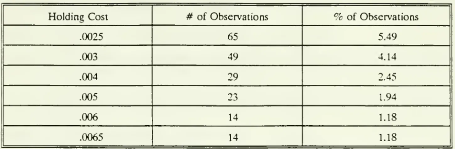
Table

I reports the

number

and percentage

of observations

which

violates the

no

arbitrage conditions for different levels ofthe

holding cost.

INSERT

TABLE

I

Table

I reveals that a

model

of holding costs alone

compares

most

favorablywith a

model

of

trading costs alone.

The

brokerage

costs estimate of

1/128%,

for both the long

and

short legs ofthe

arbitrage, plus a typical bid-ask spread of

3/32%

cited above,

would

result in 419, or

35.39%,

price

deviations

which exceed

the level of trading costs. So, holding costs

seem

to

be

quite important,

relative to trading costs, in foiling riskless arbitrage activity.

Of

course, a

model

which

incorporates

both holdingcosts

and

trading costs

does

best.

With

c

=

.006

and

these tradingcosts, forexample, only,

only 4 observations, or .34%, violate the riskless arbitrage bounds.

19

13

Returning

to the

model

of this paper, it

seemed

reasonable to settle

on

c

=

.006. This level

isin the

range

ofpriorbeliefs

and

generatesrelatively

few

violations oftheriskless arbitrage bounds.

Using

this level of holding costs

and

ignoring trading costs, figure 1 plots the individual mispricings

as a function of the riskless arbitrage

bound,

s(t).

The

two

rays are the lines

x=s

and

x=-s.:o

The

plot provides

some

additional evidence that holding costs are important inhibitors of

arbitrageactivity. Inthe

model

presentedearlier, mispricings

can

take

on

any

value

between

s(t)

and

-s(t). Consequently,

one

would

expect the variability of the mispricings to increase in s.

Looking

at

figure 1. this

seems

to be the case.

More

precisely, the standard deviation ofx is

about

.09 for

s<l,

.31 for

Ks<2,

.29 for

2<s<3,

and

.43 for

s>3.

The

next step in applying the

model

to the data at

hand

is to estimate its

parameters

_p

and

o. Recalling that d)(z)

=

z/(l+z

2₎1/2,

one

can

use (2) to transform x

and

svalues into values of the

underlying state variable, z.

Then, changes

in z can

be

regressed

on

z in order to estimate the

parameters

of the z process given by (3).21

The

results of the regression are reported in table II.

INSERT

TABLE

II

The

estimate of p is significantly negative, confirming the autoregressive nature of the

deviation process."

The

partial differential equation in (11)

can

now

be solved numerically.

Converting

the

parameters

estimated

from monthly

data to

an

annual basis gives values of

about

5.42

and

.88 for _p

and

a. respectively.

The

holding cost, c,

was

set to .6%, asdiscussed above.

The

opportunity cost of

funds, r.

was

taken to

be

9%,

a value close to the

sample

average. Finally, the original maturity of

in

' _Figure

1 alsoshowsthat the pricedeviations aremoreoftennegativethannot. Inother words,the priceof the replicating portfolio usuallyexceedsthe price of the middle bond. Thisisconsistent with a taxtimingoptionora taxclienteleeffect.See Constanunides and

Ingersoll (1984).Lilzenbergerand Rolfo(1984),and Schaefer(1982).

"'* _{Theobservations forwhich}

|x|>s were dropped from thesamplesincez is undefined in thesecases.

—

Regressing changesinxonxalso givesa significantlynegative coefficient Therefore, the functional formof$isnot responsiblefor

14

the triplet

was

set at 5 years.

The

relevant range for the underlying state variable, z, turns out to

be

well within (-2,2). In

other words, valuesofz

which

are larger inabsolute value

correspond

to mispricings

which

are larger

than those

which appear

in the data set.

Figure 2 graphs theoptimalposition sizeasa function ofzfor

two

different times to maturity.

As

predicted by Proposition 1, part i), for small mispricings it is notoptimal to take a position. Ifthe

mispricing is large

enough,

however, position size increases in the absolute value of z.

Figure 2 reveals that positionsize is not

monotonic

in time to maturity.

There

are

two

effects

at

work

here. First, since positions ofpotentially longer maturities are likely to incur larger holding

costs, investors

would

take

on

smaller positions. This might

be

called a risk effect.

Second,

since

potentially longer horizons are likelyto provide better arbitrageopportunities in the future, investors

would

be

willing to take

on

larger positions. This

might

be

called

an

option effect,

and

is related to

the

hedging

properties of

an

arbitrage position raised by claim 3.

When

z is large, realization of

current arbitrage profits is relatively

more

important than the

promise

offuture mispricings, so the

risk effect should dominate.

When

z is small,

however,

the potential of future arbitrage profits is

relatively

more

important

and

the option effect should dominate. Consequently, as

shown

in the

figure,

when

|z| is large the position size with 3.04years to maturity is greater than the position size

with 5 years to maturity.

When

|z| is small the position size with 5 years to maturity is the larger

of the two.

Although

not

shown

in the figure, the

hedging

effect described in part iii) of Proposition 1

can

be

examined through

the numerical solutions.

With

3.04 years to maturity for example, an

arbitrageur will take a position

even

when

|z|<.04.

The

instantaneous expected return

from

the

From equation (11). one only need solve for ai.wherea is the coefficient of absolute nsk aversion. Therelore.without loss ot

15

position is positive,

however,

only

when

|z|>.2. In terms ofthe dollar mispricing, x, the arbitrageur

will take a position

even

for a mispricing of less than

6

cents for every

$100

face value

bought

or

shorted.

The

expected

return over the next instant is positive,

however,

only

when

the mispricing

exceeds 31 cents

on

the

$100

position.

A

similar

comparative

static might

have

arisen with respect to o.

Larger

values ofo

make

the

arbitrage position riskier but raise the likelihood of future profit opportunities.

One

might reason,

as before, that the risk effect

would

dominate

for large mispricings while the option effect

would

dominate

for small mispricings.

As

it turns out,

however,

the

parameters determined

by the data

generate position sizes

which

increase in a: the option effect

dominates

for all relevant levels of

mispricing.

The

certaintyequivalent ofarbitrage activitycan

be

defined as the

amount one would

pay to

become

an

arbitrageurin a particulartriplet.24 Figure 3 graphs this certaintyequivalent as a function

of z for three different times to maturity.

As

expected, the certainty equivalent increases in the

absolutevalue ofz.

More

interestingly, the certaintyequivalent increases in time to maturity. It might

have

been

the case that the risk effect

would

cause the certainty equivalent to fall with time to

maturity since longer maturities run the

chance

of incurring larger holding costs.

Once

again,

however,

for the

parameters

in the Treasury market, the option effect reigns.

rv.

Conclusion

and

Suggested Extensions

This

paper

models

the effectofholdingcosts

on

the activities ofriskaverse arbitrageurs.

The

exogenous

mispricing process

was chosen

to allowprices to deviate

from fundamental

value without

allowing for riskless arbitrage opportunities. Solving for the optimal investmentpolicyofarbitrageurs

16

in such

markets

reveals behavior consistent with the casual empirical observation that professional

arbitrageurs consistently take limited arbitrage positions.

Furthermore,

a risk effect

and an

option

effect

were

identified as driving the

comparative

statics of optimal position size

and

of thevalue of

being

an

arbitrageur.

Data

from

theTreasury

bond

market supported

the

importance

of holdingcosts

in arbitrage activity, provided

parameter

estimates of the model,

and

led to

some

insights

about

the

relative

importance

ofthe risk

and

option effects.

Two

pathsoffutureresearch

emerge

from

thisanalysis. First, there is a

need

tocollectbetter

data

about

the size of holding costs in the various

markets

mentioned

in section I. Second, the

analysis of this

paper

concentrated

on

the investment

problem

facing arbitrageurs.

The

next step

would

be

to

model

the factors generating price deviations

from

fundamental

value

and

thus

endogenize

the deviation process. This

avenue

of research

would

clearly benefit

from

some

17

Appendix

1

Proof

of

PROPOSITION

1

Recall that the

Bellman

equation associated with the

CARA

arbitrageur's optimization

problem

is

F

_T

=

max, { (u

+

o

2

F

_z

)ai4o

2(ai)2 } -

pzF

z

+

lo^-F,

2 ) (11) with

u

given by u(z,t)

=

pz

- 4-o2<t>74>'

+

c(<(>-€)/s4>' (6)

and

with e being the sign of i.

The

boundary

conditions are

F(z,0)

=

0;

(Al)

F(

+

oo,_T)

=

_F(-«,t)

=

+».

(A2)

Unfortunately, condition

(A2)

is not precise

enough

to characterize the value function F(v).

Indeed

it

may

be

possible, a priori, that the arbitrageur reaches

an

unbounded

value of

F

for every

z. It is therefore necessaryto

show

that

F

can be

bounded

by thevalue function ofa control

problem

which

admits

an

explicit solution.This will

be

done

laterby the choice ofa particularfunction 4>.

For

the

moment,

assume

that the function

F

and

its derivatives are well defined

and

that <\> is a

smooth

increasing

mapping

from

(-°°.«>) into (-1.

+

1) such that 4>(-z)

=

-<J>(z).

The

symmetry

of the

problem

yields that

F(-z,t)

=

F(z,t)

(A3)

so that

F

_z(0,t)

=

for every t.

(A4)

We

can

now

proceed

with the proof of Proposition 1.

18 i(z,x)

=

i L (z,t) ifi L

(z,t)>0

(A5a)

i(z,t)

=

i s (z,t) ifi s (z,-c)<0

(A5b)

i(z,t)

=

otherwise

(A5c)

with i L (z,t)

=I-£.z-I*_-i.J_i^

+

F

7

when

i>0;

(A5d)

a

_a

2 ₂ tf 2 s(t) 4/ i s

(z,t)

=I-P-z

-1*1

+

^_L1^

*F

_wheni<0.

(A5e)

a

_o

2 ₂

<j/ 2 s(t) <j/

From

(A4), it follows that

i

L

(0,t)

<

0; i

s

(0,-r) >0.

(A6)

Therefore

i(0,t)=0and, bycontinuity, theoptimal investmentdecision forsmall mispricingsis totake

no

position. This proves i).

Proof of

ii): ii) follows

from (A5)

above.

Proof

ofHi):

From

the

symmetry

of F(z,t) with respect to z it follows that

F

z(z,t) has the

same

sign

as z. i.e. arbitrageurs are better offwith large |z|.

As

a result,

i

=

u/o

2

₊

F

_z

can be positive

even

if

u

is negative

and

vice versa.

Boundedness

ofF(z,r)

and

growth conditions:

As

mentioned

above,

growth

conditions for large z are

critical for the numerical analysis. If4>(z)=z/(l+z2₎1/2 then

i \ 3 2 z r 1+z

2

A7

,

u(z,t) =

_pz

+

_-a'

. .

(A7)

2 _1+z2

l-e

_rT f. 2

To

provide the

bounds and growth

conditions of the value function, consider a class of control

19

value function

V

M

<

->(w,z,t)

=

max,

E[U(W

_T

_)]

subject to the

dynamics

dw,

=

i

t (M(t)z,dt

- odb,)

and

dz,

=

-pz,dt

+

odb, tsT.

The

function

V

M()

can be

explicitly derived

and

is of the

form

V

m

<>(w,z,t)

=

-

exp

{-aW-F

M

()(z,t)}

where

F

M() is quadratic with respect to z:

F

m

«(z.t)

=

1k

2(t)z

:

_-K

1(t)z

^KoCt).

By symmetry

Kj(t)=0.

The

functions

K

;(t)

and

K^t)

solve the ordinary differential equations

dK«

i ,

dIC

i

,

J^

= '

_o'K.

_and

—:

= _L

M(x)

2 *

2(M(t)-

P))IC,(t)

(A8)

dt

2

dt

_a

-and

are easy to calculate.

Returning

to the original problem, observe that there exists a positive constant

M,

such that

|u(z,t)| s M|z|, for every z.

(A9)

Recalling that i,

and

z,

must have

the

same

sign, it follows that for every policy i t

dw

(

=

i, [u(z,,i)dt -

odb

t] <.

Mi

t z,dt - oi t

db

t .

(A10)

Hence

V(w,z.t) ^

V

m

(w.z,t)

<

U(«).

It follows that the control

problem

faced by the arbitrageur is

bounded

and

admits a

smooth

value function.

(See

Vila

and

Zariphopoulou

(1989)

on

proving the regularity ofthe value function

in a similar context.)

Growth

conditions can be derived by considering the

dominant term

in u(z,t) for large z.

From

(A7)

it follows that for large z, u is approximately linear in z i.e.

u(z,t) -

_(p-

_{L_)z}

=

R(t)z

.

(All)

20

Let t"

be such

that

R(t')=0.

Then

under

certain

parameter

restrictions, easily satisfied by thedata,

for every -est*

and

every z the

expected

gain u(z,t)i is nonpositive for every arbitrage position i. It

follows that the function F(z,t) = 0, for tst*.

For

t;>t\

growths

conditions are obtained by

considering the function

V

M(T)(w,z,t) with

M(t)

=

_max

{R(t);0}.

Therefore

the numerical analysis

used

the

growth

condition

1 ->

22

References

Amihud,

Y.,

and Mendelson,

H., (1991), "Liquidity, Maturity,

and

the Yields

on

U.S.

Treasury

Securities," Journal

of

Finance,

46

(4), pp. 1411-1425.

Andersen,

T., (1987),

Currency

and

Interest-Rate

Hedg

_{in g}.

New

York

Institute of Finance.

Brennan,

M.,

and

Schwartz, M., (1990), "Arbitrage in Stock

Index

Futures,"_{Journal of}Business,vol.

63(1), pt. 2, pp. s7-31.

Constantinides,

G. and

Ingersoll, J., (1984), "Optimal

Bond

Trading

with Personal Taxes." Journal

of

Financial

Economics,

13, pp. 299-335.

Cox. J.,

and

Rubinstein, M., (1985),

Options Markets

. Prentice-Hall, Inc.

De

Long,

J. B.,

A

Shleifer, L.H.

Summers,

and

R. J.

Waldmann,

1990,

Noise

trader risk in financial markets.Journal

of

Political

Economy

98, 703-738.

Dumas,

B.,

and

Luciano, E., (1991),

"An

Exact Solution to the Portfolio

Choice

Problem

Under

Transactions Costs,"Journal

of

Finance, 46(2), pp. 577-595.

Duffle, D., (1989), Futures

Markets

, Prentice-Hall. Inc.

Fleming, W.,

Grossman,

S.,Vila,J.L.,

Zariphopoulou,

T,

(1989),

"Optimal

Portfolio

Rebalancing

with Transaction Costs," unpublished manuscript.

Grossman,

S.,

and

Vila, J.L., (1989), "Optimal

Dynamic

Trading

with

Leverage

Constraints."Journal

of

Financial

and

Quantitative Analysis, (forthcoming).

Hodges,

S..

and

Neuberger,

A,

(1989) "Optimal Replication of

Contingent

Claims

Under

Transactions Costs,"

The Review

of Futures Markets, vol. 8(2), pp. 222-242.

Holden.

C,

(1990),

"A Theory

of Arbitrage

Trading

in Financial

Market

Equilibrium," Discussion

Paper #478,

Indiana University.

Lee,

CM.,

A

Shleifer

and

R. H. Thaler. 1991, Investor

Sentiment and

the

Closed-End

Fund

Puzzle.

Journal

of

Finance, 46, 75-109.

Litzenberger, R.,

and

Rolfo,J., (1984),"ArbitragePricing, Transactions Costs

and

Taxation ofCapital Gains,"Journal of Financial

Economics,

13. pp. 337-351.

Merton,

R., (1973),

"An

Intertemporal Capital Asset Pricing

Model,"

Econometrica, vol. 41. _pp. 867-887.

23

of Paul H. Cootner. Sharper, W.,

and

Cootner,

C,

eds., Prentice Hall. pp. 159-178.

Schwartz, E.. Hill, J.,

and

Schneeweis, E., (1986), Financial Futures,

Richard

Irwin. Inc.

Stigum, M., (1983),

The

Money

Market, 2nd

edition,

Dow

Jones-Irwin.

Stigum, M., (1990),

The

Money

Market,

3rd edition,

Dow

Jones-Irwin.

Vila, J.L.,

and

Zariphopoulou.

T., (1989),

"Optimal

Consumption

and

Portfolio

Choice

with

24

Table

I

Frequency

of riskless arbitrage

bound

violations as a function of the level ofholding costs

Table

I reports the

number

and

percentage of observations

which

violates the

no

arbitrage

condition |x,|<s(t) for different levels of the holding cost.

There

are

1184

observations in all.

25

Table

II

OLS

regression results

from

estimating the process

dz

=

-pzdt

+

odb

with

monthly

observations.

Zt₊l " *!

=

P2!

+

€t

p

=

-.452

The

regression

model

is:

with 1125 observations.

The

estimated value of p is:

with a standard error of.0257.

The

R

squared

is:

R

2

₌

.216

The

estimated value of

a

is taken to be the standard error of the residuals:

Figure 1

$ Mispricing per

$100 Face

Value

co rb ro CO

-Figure 2

Position Size

in

Face

Value

(Thousands)

a*

o

en

O

o

CO

o

O

O

O

O

CO

O

O

cn

O

(J)

O

c

D

Q. CD

<

5' CO C/5 r+ 0) CD

<

Q) Q)' C£ CO

N

Figure 3

Date

Duef

-fr-*

,11 UBRARItS