Vehicle routing problems with multiple trips

HAL Id: emse-01250603

https://hal-emse.ccsd.cnrs.fr/emse-01250603

Submitted on 3 Feb 2016

HAL is a multi-disciplinary open access

archive for the deposit and dissemination of sci-entific research documents, whether they are pub-lished or not. The documents may come from teaching and research institutions in France or abroad, or from public or private research centers.

L’archive ouverte pluridisciplinaire HAL, est destinée au dépôt et à la diffusion de documents scientifiques de niveau recherche, publiés ou non, émanant des établissements d’enseignement et de recherche français ou étrangers, des laboratoires publics ou privés.

Vehicle routing problems with multiple trips

Diego Cattaruzza, Nabil Absi, Dominique Feillet

To cite this version:

Diego Cattaruzza, Nabil Absi, Dominique Feillet. Vehicle routing problems with multiple trips. 4OR: A Quarterly Journal of Operations Research, Springer Verlag, 2016, 14 (3), pp.223-259. �10.1007/s10288-016-0306-2�. �emse-01250603�

Vehicle routing problems with multiple trips

Diego Cattaruzza

, Nabil Absi

, and Dominique Feillet

1

_{Univ. Lille, CNRS, Centrale Lille, UMR 9189 - CRIStAL - Centre de Recherche}

en Informatique Signal et Automatique de Lille, F-59000 Lille, France , Tel.:

+33-3-20335494

2,3

_{Ecole des Mines de Saint-Etienne and LIMOS UMR CNRS 6158, CMP Georges}

Charpak, F-13541 Gardanne, France

Abstract

This paper presents a survey on the Multi-Trip Vehicle Routing Problem (MTVRP) and on related routing problems where vehicles are allowed to perform multiple trips. The first part of the paper focuses on the MTVRP. It gives an unified view on mathematical formulations and surveys exact and heuristic approaches. The paper continues with variants of the MTVRP and other families of routing problems where multiple trips are sometimes allowed. For the latter, it specially insists on the motivations for having multiple trips and the algorithmic consequences. The expected contribution of the survey is to give a comprehensive overview on a structural property of routing problems that has seen a strongly growing interest in the last few years and that has been investigated in very different areas of the routing literature.

1

Introduction

Since the introduction of the Vehicle Routing Problem (VRP) by Dantzig and Ramser in 1959 [40], the vast majority of papers interested in vehicle route optimization share the same assumption (largely realistic in practice) that each vehicle is restricted to perform at most one trip. The first visible attempt to address a vehicle routing problem with multiple trips dates back from Fleischmann [44] under the name Vehicle Routing Problem with Multiple Use of Vehicles, in the context of the solution of a series of distribution problems involving a heterogeneous fleet of vehicles and time windows (see Section 3).

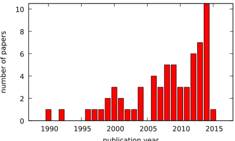
Despite the clear improvements that could be obtained, in some situations, by allowing vehicles to perform multiple trips, this feature remained very punctually investigated for years. However, a significant increase of the number of publications dealing with this subject can be observed in the recent literature, as shown in Figure 1. One important reason for this gain of interest is the development of new distribution schemes in cities. Nuisances related to congestion and pollution pushed scholars, communities and enterprises to study new delivery policies to increase city livability. Common approaches envisage the use of electrical vehicles and/or forbid heavy trucks to enter city centers. Moreover, physical city structures often force final deliveries to be accomplished by small-sized vans that can go through narrow streets.

The usage of electrical vehicles or small-sized vans ends up in delivery trips shorter than the working day due to, respectively, limited autonomy and capacity. Unless multiple trips are allowed for vehicles, a consequence is the bad exploitation of the time horizon and the need of an oversized fleet to satisfy all the customers (Cattaruzza et al. [22]). Operations, then, assume the possibility to

0 2 4 6 8 10 1990 1995 2000 2005 2010 2015 number of papers publication year

Figure 1 – Number of publications per year cited in this survey and dealing with multi-trip trans-portation (PhD theses excluded)

re-load vans when they are back at the depot and route them for another trip. As it will be seen in the subsequent sections, many other sources of motivation can however be found, in domains as far to city logistics as maritime transportation.

The aim of this survey is to give a clear overview of the work devoted to vehicle routing problems with multiple trips, and to highlight how the possibility to link up several trips for a vehicle impacts solution methods.

An important difficulty to meet our goal was the naming of these problems. The Multi-Trip Vehicle Routing Problem (MTVRP) appears in the literature under several names. In addition to the already mentioned VRP with multiple use of vehicles used by Fleischmann [44], it has been addressed as multitrip VRP (Prins [72]), VRP with multiple routes (Azi et al. [8]), VRP with multiple trips (Olivera and Viera [66]), VRP with multiple depot returns (Tsirimpas et al. [89]) and multiple trip VRP (Battarra et al. [12]). Taniguchi and Van Der Heijden [87] allow vehicles to make multiple traverses, while the multiple usage of vehicles has been called recycling of trucks in Van Buer et al. [92]. The differences in the problem naming, made the research of papers difficult. Moreover, several works dealing with multi-trip routing problems do not mention this aspect in the title, nor in the abstract, making the hunt even harder. For this reason there could probably be some fishes that escaped our net.

A previous literature review was proposed by S¸en and B¨ulb¨ul [39] but with a very limited scope: only the pure MTVRP was surveyed. In this paper we address a broader class of problems, whose limits are precisely defined in the next paragraphs. However, before making clear the class of problems we consider, we need to clarify some terminology.

All along the paper we refer to a trip as a sequence of customer services preceded and followed by a visit to a depot and without intermediate stop at a depot. Note that the empty trip is included in this definition. A sequence of trips performed by the same vehicle is called journey. Note that the definitions of trip and journey are not limited to the single-depot case, i.e., the starting and the ending depots can differ if the problem involves several depots. In the literature trip and journey can, for example, be respectively referred to trip and tour, tour and multi-tour (Aghezzaf et al. [2]), route and schedule (Mingozzi et al. [62]) or to voyage and route (in maritime context, Section 3.3). To further clarify, we say that a problem involves the multi-trip aspect, when vehicles have the possibility to accomplish, during the same working day, journeys made by more than one trip.

Stochastic routing problems where returns to the depot can be implied by recourse strategies are not considered in this survey. In these problems, anticipated returns to the depot result from the realization of the uncertainty, for example because of underestimated demands. However, since these returns are not part of the initial plan, we decided to exclude this category of problems from

the survey. Similarly, several papers deal with special routing problems, where the weight of routing decisions is very limited. An example is given by Ronen [78] that considers multiple trips in Full Truckload distribution. Another example is found in Tsirimpas et al. [89], where the optimization of an automated guided vehicle system along fixed paths is addressed. These papers are also excluded from the survey.

On the contrary, we decided to include multi-trip routing problems where the fleet is composed of a single vehicle. In the VRP literature the single vehicle case (Traveling Salesman Problem, Gutin and Punnen [50]) and the multi-vehicle case (VRP, Toth and Vigo [88]) are usually distinguished because of the strong differences between these problems (one can just look at the largest instances solved exactly for these two problems to be convinced). When multiple trips are allowed, a single-vehicle solution has the same characteristics as a VRP solution and we believe that this case thus deserves to be part of this survey.

The paper is structured as follows. In Section 2 we introduce the MTVRP and survey the related literature. Section 3 deals with important variants of the MTVRP. The section is decomposed in five subsections. In Subsection 3.1, we present direct extensions of the MTVRP for which benchmarks exist and an on-going “horse race” is run. Subsection 3.2 is devoted to multiple trips in the context of combined routing, production and/or inventory optimization. In Subsection 3.3, we focus on multi-trip routing in the context of maritime transportation. Subsection 3.4 investigates multi-multi-trip vehicle routing in the context of multi-level distribution. This section is finally concluded with Subsection 3.5, where other types of constraints met in multi-trip vehicle routing problems are reviewed. Section 4 concludes the paper.

2

The Multi-Trip Vehicle Routing Problem

As explained above, the Multi-Trip Vehicle Routing Problem was introduced in different papers, under different names and sometimes with some slight differences in the definition. We propose here to retain the following definition.

Let G = (N , A) be a directed graph, where N = {0, 1, . . . , N } is the set of nodes and A = {(i, j)|i, j ∈ N } is the set of arcs. Arcs (i, j) ∈ A are characterized by their travel time Tij. Node 0

represents the depot where a fleet V of identical vehicles with limited capacity Q is available at time 0 and has to be returned at time TH. Nodes 1, . . . , N represent the customers to be served, each one

requiring a certain non-negative quantity Qi of a product. The MTVRP calls for the determination

of a set of trips and an assignment of each trip to a vehicle, such that the traveled time is minimized and the following conditions are satisfied:

(i) each trip starts and ends at the depot,

(ii) each customer is visited exactly once,

(iii) the sum of the demands of the customers in any trip does not exceed Q,

(iv) the sum of the durations of the trips assigned to the same vehicle (journey) does not exceed TH (a trip duration being the sum of the travel times on arcs used in the trip).

Note that vehicles are not necessarily all used. In papers on the pure MTVRP, loading times are not introduced. Service times are sometimes included (e.g., Taillard et al. [85]), sometimes not (e.g., Olivera and Viera [66]). In the benchmark instances issued from Taillard et al. [85] (see Subsection 2.2), they are set to zero. For this reason we did not include service times nor loading times in this definition. Note that one can however consider them being included in the travel time matrix.

In most papers (and in the aforementioned instances), the travel time matrix is symmetric. The problem can then indifferently be defined on a directed or an undirected graph. Depending on the

papers, one of this two options is chosen. To be as general as possible, and following usual trends when time is part of the problem definition (and induces an implicit orientation of routes), we decided to define the MTVRP on a directed graph. As far as we can see in the surveyed literature, the issue of the travel time matrix being symmetric or not is not a major issue.

Olivera and Viera [66] shortly prove that the MTVRP is N P-hard as being a generalization of the VRP. Quoting Olivera and Viera [66], “any VRP instance can be transformed to an equivalent MTVRP instance, setting |V| = N and TH = P_(i,j)∈Atij”. Apart from this short proof, we did

not find any discussion on the complexity of the MTVRP in the literature. Implicitly, the proof by Olivera and Viera [66] assumes that an unlimited fleet of vehicles is available in the VRP. We propose below a more formal proof, where this assumption is removed.

Proposition 1. The MTVRP is an N P-hard problem

Proof. We prove it by reduction to the VRP. Given a VRP instance, we duplicate it to construct a MTVRP instance where: (i) parameter TH is added and is set to 2 ×

P

(i,j)∈ATij and, (ii) travel

times on arcs returning to the depot are increased by TH

2 . Note that no vehicle can perform more

than one trip in this MTVRP instance. The solution sets of the VRP and MTVRP instances are identical, with identical cost evaluation functions. Seeing that the VRP is N P-hard (Lenstra and Rinnooy Kan [58]), it proves that the MTVRP is N P-hard.

2.1

Mathematical formulations for the MTVRP

As far as we know, the only compact formulation proposed for the MTVRP is by Koc and Karaoglan [55]. However, several very different formulations exist for extensions of the MTVRP, from which formulations can be deduced for the MTVRP. We review these formulations below. We exclude extended formulations that are discussed in Section 2.3.

For the sake of consistency, we sometimes slightly modify the models found in the papers (in addition to removing all the variables and constraints that do not relate to the MTVRP). In these models, M represents a large enough constant. The objective in this section is not to compare these formulations (information is lacking) but rather to present an unified view of the literature.

4-index formulations

The most common formulation is an extension of the 3-index vehicle flow formulation (3VFF-VRP) initially introduced for the VRP, where a fourth index is added for trips. In this formulation a pair composed of a trip and the vehicle that performs this trip exactly plays the role played by a vehicle in 3VFF-VRP. All constraints from the 3VFF-VRP can thus just be translated. An additional constraint is needed in order to limit the total duration of the journey for each vehicle.

A limit of this formulation is that the number of trips that can be envisaged for each vehicle is unknown. An easy upper bound is N , but it then conducts to a very weak formulation with a large number of variables. In some papers where the maximal number of trips per vehicle is bounded, this limit is withdrawn. We present this 4-index formulation below, adapted from the 3VFF-VRP given in Chapter 1 of Toth and Vigo [88]. It relies on the following decision variables:

xvr_ij = (

1 if trip r ∈ R of vehicle v ∈ V travels through arc (i, j) ∈ A, 0 otherwise,

y_ivr = (

1 if trip r ∈ R of vehicle v ∈ V visits vertex i ∈ N , 0 otherwise,

where R = {0, . . . , N − 1}. The model is then as follows: min X (i,j)∈A Tij X v∈V X r∈R xvr_ij (1) s.t. X v∈V X r∈R y_ivr = 1 ∀i ∈ N \ {0}, (2) X j∈N xvr_ij =X j∈N xvr_ji = y_ivr ∀i ∈ N , v ∈ V, r ∈ R, (3) X i∈N \{0} Qiyvri ≤ Q ∀v ∈ V, r ∈ R, (4) X i∈S X j∈S xvr_ij ≤ |S| − 1 ∀S ⊆ N \ {0}, |S| ≥ 2, v ∈ V, r ∈ R, (5) X r∈R X (i,j)∈A Tijxvrij ≤ TH ∀v ∈ V, (6) xrv_ij ∈ {0, 1} ∀v ∈ V, r ∈ R, (i, j) ∈ A, (7) y_irv ∈ {0, 1} ∀v ∈ V, r ∈ R, i ∈ N . (8) Constraints (1)-(5) are taken from Toth and Vigo [88]. Constraints (6) limit to TH each vehicle’s

journey. Trip index on xvr_ij variables is needed because of capacity constraints (4). Vehicle index is needed because of constraint set (6) and because the fleet size is limited (one cannot simply bound the outgoing flow from the depot to limit the number of vehicles used, because of the multi-trip feature). To the best of our knowledge, the first appearance of this formulation dates back from 2006, in Gribkovskaia et al. [49], for a complex livestock collection problem. Since then, several authors proposed the same type of formulation (e.g., Azi et al. [8], Alonso et al. [3]).

Lei et al. [57] propose a different 4-index formulation extended from the single-commodity flow formulation of the VRP (Toth and Vigo [88]). In this formulation, flow variables qvr

ij are added and

represent the load in vehicle v when traversing arc (i, j) during its trip r. Constraints (4)-(5) are then replaced with:

X j∈N q_jivr−X j∈N qvr_ij = Qi ∀i ∈ N \ {0}, v ∈ V, r ∈ R, (9) q_ijvr ≤ Qxvr ij ∀(i, j) ∈ A, v ∈ V, r ∈ R, (10) qvr_ij ≥ 0 ∀(i, j) ∈ A, v ∈ V, r ∈ R. (11) Note that these constraints manage both vehicle capacity and subtour elimination.

3-index formulations with vehicle index (without trip index)

Surprisingly, Lei et al. [57] conserved the trip index in the above formulation while it is apparently not necessary anymore. Actually, Aghezzaf et al. [2] propose an equivalent formulation where the trip index is removed:

min X (i,j)∈A Tij X v∈V xv_ij (12)

s.t. X v∈V y_iv = 1 ∀i ∈ N \ {0}, (13) X j∈N xv_ij =X j∈N xv_ji= yv_i ∀i ∈ N , v ∈ V, (14) X j∈N q_jiv −X j∈N q_ijv = Qi ∀i ∈ N \ {0}, v ∈ V, (15) q_ijv ≤ Qxv ij ∀(i, j) ∈ A, v ∈ V, (16) X (i,j)∈A Tijxvij ≤ TH ∀v ∈ V, (17) xv_ij ∈ {0, 1} ∀v ∈ V, (i, j) ∈ A, (18) y_iv ∈ {0, 1} ∀v ∈ V, i ∈ N , (19) q_ijv ≥ 0 ∀(i, j) ∈ A, v ∈ V. (20) Constraints (12)-(14) and (17) come from (1)-(3) and (6), respectively. Constraints (15)-(16) come from (9)-(10).

Coming back to vehicle flow formulations, Buhrkal et al. [18] propose a 3-index formulation extended from the 2-index vehicle flow formulation of the VRP. To get rid of the trip index, capacity constraints are expressed using Miller-Tucker-Zemlin-like constraints [61]. The resulting formulation is similar to (12)-(20), replacing (15)-(16),(20) with:

q_iv+ Qi ≤ qjv+ Q(1 − x v

ij) ∀i ∈ N \ {0}, j ∈ N , v ∈ V, (21)

0 ≤ q_iv ≤ Q ∀i ∈ N , v ∈ V, (22) where qv

i represents the accumulative load in vehicle v before serving customer i. Note that these

constraints also eliminate subtours.

In both formulations, the vehicle index is kept because of constraints (17) and the limited fleet size.

3-index formulations with trip index (without vehicle index)

Two 3-index formulations have been proposed where the vehicle index is removed instead of the trip index (Azi et al. [9], Hernandez et al. [54]). As stated above, the difficulty is then to handle the time-horizon constraint and the size of the fleet.

In Azi et al. [9], the problem addressed involves time windows and time variables tr

i are present:

tr_i indicates the time at which trip r visits customer i, if i is visited in r, 0 otherwise; tr₀ indicates the starting time of trip r; tr

N +1 indicates its ending time. These variables are needed when translating

the model to the MTVRP, even if the time windows are removed. New binary variables zrs (with

r < s) are also introduced to detect consecutive trips: zrs= 1 if and only if trip r is followed by trip

s on the same vehicle. The resulting model is:

min X (i,j)∈A Tij X r∈R xr_ij (23)

s.t. X r∈R yr_i = 1 ∀i ∈ N \ {0}, (24) X j∈N xr_ij =X j∈N xr_ji = y_ir ∀i ∈ N , r ∈ R, (25) X i∈N \{0} Qiyir ≤ Q ∀r ∈ R, (26) tr_i + Tij ≤ trj + M (1 − x r ij) ∀i ∈ N , j ∈ N \ {0}, r ∈ R, (27) tr_i + Ti0 ≤ trN +1+ M (1 − x r i0) ∀i ∈ N \ {0}, r ∈ R, (28) tr_{N +1}≤ ts₀+ M (1 − zrs) ∀r, s ∈ R, r < s, (29) tr_{N +1}≤ TH ∀r ∈ R, (30) |R| −X r∈R X s∈R,r<s zrs≤ |V| , (31) X r∈R,r<s zrs ≤ 1 ∀s ∈ R, (32) X r∈R,s<r zsr ≤ 1 ∀s ∈ R, (33) xr_ij ∈ {0, 1} ∀r ∈ R, (i, j) ∈ A, (34) yr_i ∈ {0, 1} ∀r ∈ R, i ∈ N , (35) tr_i ≥ 0 ∀r ∈ R, i ∈ N ∪ {N + 1}, (36) zrs ∈ {0, 1} ∀r, s ∈ R, r < s. (37)

Constraints (23)-(26) correspond to (1)-(4). Time variables are computed with constraints (27)-(29) The time-horizon constraint is expressed with constraints (30). Constraints (31) are added to limit the number of vehicles. The left-hand side of the constraint indicates the number of vehicles used, based on the observation that the number of consecutive trips in a journey is equal to the number of trips in the journey minus one. Constraints (32) and (33) prevent variables zrsfrom being artificially

set to one. They are needed to make sure that the left-hand side of Constraint (31) indeed represents the number of vehicle used. Note that these two constraints are forgotten in Azi et al. [9].

Hernandez et al. [54] propose an alternative for constraints (31)-(33). They replace binary variables zrs with variables zrsv such that zrsv = 1 when r is scheduled before s on vehicle v (note

that these variables are defined for all r, s ∈ R and that they are equal to 1 even if r and s are not consecutive). They introduce binary variables σv

r where σrv = 1 indicates that a trip r is assigned to

a vehicle v. Constraints (29), (31)-(33), (37) are replaced with:

tr_{N +1}≤ ts₀+ M (1 − z_rsv ) ∀v ∈ V, r, s ∈ R, r 6= s (38) 1 − z_rsv − zv sr ≥ 0 ∀v ∈ V, r, s ∈ R, r 6= s, (39) X v∈V σv_r = y₀r ∀r ∈ R, (40) σ_rv+ σv_s ≤ 1 + zv rs+ z v sr ∀v ∈ V, r, s ∈ R, r 6= s, (41) z_rsv ∈ {0, 1} v ∈ V, r, s ∈ R, r 6= s, (42) σ_rv ∈ {0, 1} ∀v ∈ V, r ∈ R. (43) Constraints (38) come from (29). Constraints (39) impose an order between trips assigned to the same vehicle. The assignment of trips to vehicles (variables σ_rv) is managed with constraints (40). Constraints (41) are coupling constraints.

2-index formulations (without vehicle index nor trip index)

Finally, two two-index formulations were also proposed by Koc and Karaoglan [55] and Rivera et al. [76].

In Koc and Karaoglan [55], binary variables x0_ij are introduced to detect when a trip finishing with customer i is followed (on the same vehicle and after a stop at the depot) by a trip visiting j as first customer (x0_ij = 1). The role played by these variables is very similar to the role played by variables zrs in the 3-index formulation proposed by Azi et al. [9], and so are the constraints

involved. min X (i,j)∈A Tijxij (44) s.t. X j∈N xij = 1 ∀i ∈ N \ {0}, (45) X j∈N xij = X j∈N xji ∀i ∈ N , (46) qi+ Qi ≤ qj + Q(1 − xij) ∀i ∈ N \ {0}, j ∈ N , (47) ti+ Tij ≤ tj + M (1 − xij) ∀i ∈ N , j ∈ N \ {0}, (48) ti+ (Ti0+ T0j) ≤ tj + M (1 − x0ij) ∀i, j ∈ N \ {0}, (49) T0i≤ ti ≤ TH − Ti0 ∀i ∈ N \ {0}, (50) X j∈N \{0} x0_ij ≤ xi0 ∀i ∈ N \ {0}, (51) X i∈N \{0} x0_ij ≤ x0j ∀j ∈ N \ {0}, (52) X j∈N \{0} x0j − X i∈N \{0} X j∈N \{0} x0_ij ≤ |V| , (53) xij ∈ {0, 1} ∀(i, j) ∈ A, (54) x0_ij ∈ {0, 1} ∀i, j ∈ N \ {0}, (55) 0 ≤ qi ≤ Q ∀i ∈ N , (56) ti ≥ 0 ∀i ∈ N \ {0}, (57)

Note that in this formulation yi variables are not introduced anymore, because they would directly

be constrained to 1. Note also that variable t0 is not introduced. The objective function (44)

corresponds to (1), while Constraints (45)-(46) correspond to (2)-(3). Capacity constraints (47),(56) are equivalent to (21)-(22). Constraints (48) participate to the computation of visiting times and are equivalent to (27). Constraints (49)-(50) complete the computation of time variables and impose finishing journeys before the end of the time horizon. Constraints (53) impose the fixation of variables x0_ij to satisfy the fleet size. Constraints (51)-(52) then connect these variables with returns to the depot.

Rivera et al. [76] propose a formulation based on the same type of variables, but instead of coming back to the depot between two consecutive trips, vehicles use replenishment arcs that have been added to the graph. Variables x0_ij then represent the flow on these arcs. Constraints (51)-(52)

are removed, constraints (45)-(46) are replaced by X j∈N xij+ X j∈N \{0} x0_ij = 1 ∀i ∈ N \ {0}, (58) X j∈N xji+ X j∈N \{0} x0_ji = 1 ∀i ∈ N \ {0}, (59)

and constraints (53) are replaced by

X

i∈N \{0}

x0i ≤ |V| . (60)

Note that in addition capacity constraints are managed with a single-commodity flow formulation (see Constraints (9)-(11)). Constraints (47),(56) are then changed to:

X j∈N qji− X j∈N qij = Qi ∀i ∈ N \ {0}, (61) qij ≤ Qxij ∀i ∈ N \ {0}, j ∈ N , (62) q0j ≤ Q(x0j + X i∈N \{0} x0_ij) ∀j ∈ N \ {0}, (63) qij ≥ 0 ∀(i, j) ∈ A. (64)

2.2

Instances for the MTVRP

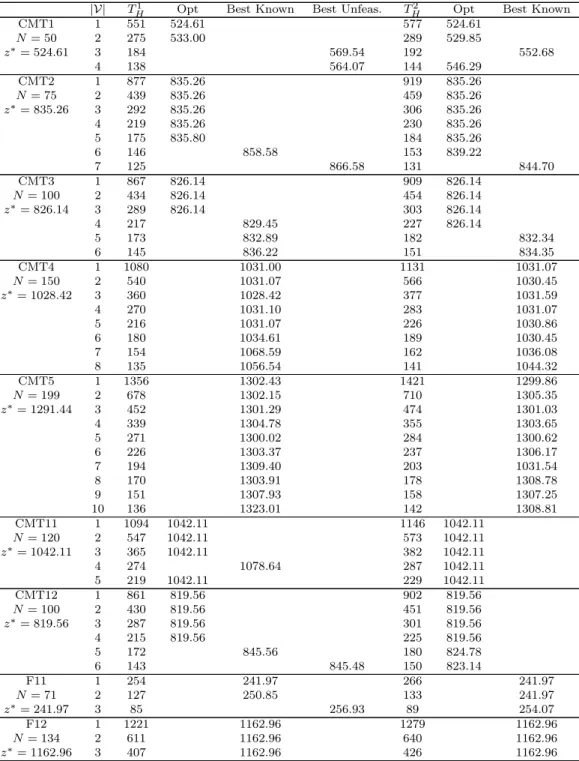
The benchmark of instances for the MTVRP was introduced in Taillard et al. [85] and is constructed from the instances 1–5 and 11–12 proposed by Christofides et al. [29] (usually denoted CMT1– CMT5 and CMT11–CMT12) and instances 11–12 proposed by Fisher [43] (F11-F12) for the VRP. All these instances are Euclidean: customer locations are described with coordinates and travel times computed accordingly. As a consequence the triangle inequality is satisfied.

From each VRP instance, several instances are constructed with different values for the number of available vehicles |V| and two different values for the time horizons TH, given by TH1 =

h 1.05z∗ |V| i and T2 H = h 1.1z∗ |V| i

where z∗ is the solution cost of the original VRP instance found by Rochat and Taillard [77] and [x] represents the closest integer to x. It results in a benchmark set of 104 instances. Surprisingly, Taillard et al. [85] adopted the following convention when reporting their experi-ments. First, they changed the problem definition by allowing overtime, penalized by a factor 2. Then, they only reported solution costs when they were not able to find a feasible solution. When a feasible solution was found, they just indicated it. Note that in this case, unfeasible solutions can cost less than feasible solution. Aside from a few exceptions, next researchers followed the same scheme.

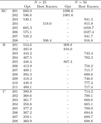
Optimal solutions are known for 42 out of the 104 instances. Feasible solutions have been found for all remaining instances except for 5. Optimal and best known solution values on this benchmark set are reported in Appendix A. For the 5 instances for which no feasible solution has been found, the cost including the penalty for overtime is given.

One can observe from the results given in Appendix A that for all instances but 7 for which the optimal solution is known (that is 35 out of 42), the value obtained is equal to z∗. When |V| = 1 it is not surprising as it is a direct consequence of the way the instances are constructed: the optimal VRP solution can be interpreted as a set of trips assigned to the single vehicle involved in the instance. When, |V| > 1 it tends to indicate that the routes present in the optimal VRP solution can in many cases be combined to form feasible journeys. It also means that a solution method able to first

find the optimal VRP solution and then to find an optimal assignment of the trips obtained to the vehicles, would certainly obtain many optimal solutions. Actually, next sections will show that it is a scheme that has been followed by many researchers. A second observation that can be made from these results, is that when the number of vehicles increases (and the horizon decreases), solution costs tend to increase and it seems more difficult to find optimal or even feasible solutions. It probably means that the packing of trips into vehicles is more challenging and that the two components of the problem (construction of trips and packing of these trips) are more deeply interlinked.

We review in the following subsections the solution algorithms proposed for the MTVRP. We restrict ourselves to algorithms that present numerical results on the above instances, which is the case for all papers addressing the pure MTVRP plus a few papers that tackled more general problems.

2.3

Exact methods

The first exact method we are aware is by Koc and Karaoglan [55]. They propose a branch-and-cut algorithm where cuts are valid inequalities taken from the VRP literature that remain valid for the MTVRP. They propose preliminary results limited to the 8 instances constructed from CMT1 in the benchmark set (50 customers) and are able to find 3 optimal solutions.

Mingozzi et al. [62] propose a much more sophisticated exact method based on branch-and-price. This method extends previous works from the same authors applied to the VRP and variants. It combines two set partitioning formulations. The first formulation defines columns as trips. The master problem is then in charge of selecting trips and combining them to form journeys. The second formulation defines columns as journeys. The master problem then only has to select journeys. These two formulations are successively used to compute the best possible lower bound. It is interesting to note that in the first formulation the pricing problem is very similar to what can usually be found when applying branch-and-price to vehicle routing problems, while it is the master problem for the second formulation. This algorithm is able to find an optimal solution for 42 instances, the ones indicated above for which the optimal solution is known.

Note there are some inconsistencies between the branch-and-cut method by Koc and Karaoglan [55] and the branch-and-price method by Mingozzi et al. [62]. Indeed, Koc and Karaoglan [55] report an upper bound on instance CMT1, |V| = 4, TH = 144 lower than the optimal solution value reported

later by Mingozzi et al. [62].

2.4

Heuristics

The first heuristic approach for the MTVRP can be found in Taillard et al. [85]. They propose a two-phase algorithm. In the first phase, several VRP solutions are created and the trips forming these solution are inserted in a list. In the second phase, MTVRP solutions are constructed with a Bin Packing Problem (BPP) heuristic where the trips are the objects to be packed into bins with capacity equal to TH. Once a trip is selected from the list, trips serving the same customers are discarded.

The VRP solutions of the first phase are built using a tabu search algorithm with adaptive memory (Taillard [84]). The BPP heuristic is a simple greedy algorithm completed with swaps of trips.

Petch and Salhi [70] reproduce this two-phase scheme but completes it with a third phase improv-ing the MTVRP solutions found. In the first phase, VRP solutions are obtained from two sources: a parametric savings algorithm (Yellow [94]) and a sweep approach. The second phase is carried out with a simple BPP heuristic similar to the one used in Taillard et al. [85]. Compared to Taillard et al. [85], the effort made in these two phases is very limited, which explains (and is explained by) the third phase.

The authors propose several components to improve the MTVRP solutions in the third phase. First, they introduce an original local search operator defined as follows:

• one of the two resulting trips is moved to another vehicle.

Note that this operator cannot improve the length of the trips (as long as the triangle inequality is satisfied) but can contribute to a better packing (decreasing overtime). In addition, a standard VRP local search is applied to each vehicle separately, by addressing the trips forming the journey of a vehicle as a VRP solution. Finally, this local search is completed with attempts of reallocation of customers between vehicles.

Other authors abandon this principle of a two-phase algorithm focusing first on VRP solutions. Instead, they apply and adapt existing metaheuristic schemes to the MTVRP.

Several authors propose tabu search (TS) algorithms. Brand˜ao and Mercer [17] adapt to the MTVRP a TS algorithm initially designed for a practical problem involving multi-trip vehicle routes (Brand˜ao and Mercer [17]). Alonso et al. [3] propose a TS approach for a periodic MTVRP. In both cases, the algorithm uses standard VRP local search operators. Apart from the construction of the initial solutions, the fact that multiple trips are assigned to vehicles only influences the evaluation of the solutions with regard to overtime.

Olivera and Viera [66] follow Taillard et al. [85] by using a TS algorithm with adaptive memory, but applying the approach to MTVRP solutions. As usual in TS with adaptive memory, the memory is composed of trips. When a set of trips is selected to form a new VRP solution, this solution is changed to a MTVRP solution with a BPP heuristic. Then, after each move of the TS algorithm, the BPP heuristic is repeated to search for better assignment of the trips to the vehicles. The local search operators used in the TS are standard VRP local search operators that move customers between trips: no operator can change the assignment of trips to vehicles.

Salhi and Petch [80] address the problem with a genetic algorithm, completed with local search. In this method a chromosome is a sequence of strictly increasing angles, measured with respect to the depot, and dividing the plane into sectors. Chromosomes are decoded as follows: customers are assigned to the sector they occupy; in each cluster, the Clarke and Wright [31] savings heuristic is applied; the resulting VRP solution is finally transformed to a MTVRP solution with a BPP heuristic. Local search is managed as in Petch and Salhi [70].

Cattaruzza et al. [21] also propose a population-based algorithm. They apply the giant tour coding popularized by Prins [73]. To decode chromosomes, they first execute the split procedure initially proposed by Prins [73] for the VRP. They then compute by dynamic programming the best MTVRP solution that can be obtained with the trips of this solution. Local search is composed of standard VRP local search operators improved with what the authors call combined local search. They observe that completing a move with a swap of trips can make beneficial a non-beneficial move. They propose several rules to apply these combined moves with a limited impact on computing times. Note that the local search operator introduced by Petch and Salhi [70] can be seen as an example of combined move.

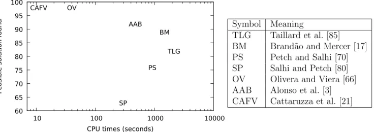
Figure 2 gives algorithm comparison. The reported CPU times are the original ones: no scale factor is considered. The machines used to run the algorithms are reported in Table 1. State-of-the-art algorithms are provided by Olivera and Viera [66], Cattaruzza et al. [21]. Detailed algorithm comparison can be found in Cattaruzza et al. [21]. The algorithm proposed by Alonso et al. [3] is proposed to solve a richer problem that considers a multi-period horizon and accessibility constraints.

3

Variants of the MTVRP

This section surveys several important categories of routing problems with multiple trips. The first category (Section 3.1) consists of direct (academic) extensions of the MTVRP for which benchmarks exist and are subject to competition between authors. This section contains two other papers (Anaya-Arenas et al. [4] and Chbichib et al. [25]) that are not involved in this competition but address the same problems motivated by a real-life application. The second category consists of complex routing,

60 65 70 75 80 85 90 95 100 10 100 1000 10000

Feasible solution found

CPU times (seconds)

TLG BM PS SP OV AAB CAFV Symbol Meaning TLG Taillard et al. [85]

BM Brand˜ao and Mercer [17] PS Petch and Salhi [70] SP Salhi and Petch [80] OV Olivera and Viera [66] AAB Alonso et al. [3] CAFV Cattaruzza et al. [21]

Figure 2 – Algorithm comparison on benchmark instances

Paper Machine RAM

TLG 100 Mhz Silicon Graphics Indingo -BM HP Vectra XU Pentium Pro 200 Mhz -PS Ultra Enterprise 450 dual processor 300 Mhz -SP Ultra Enterprise 450 dual processor 300 Mhz

-OV 1.8 Ghz AMD Athlon XP 2200+ 480 Mb AAB DELL Dimensio 8200 1.6 Ghz 256 Mb CAFV Intel Xeon 2.8 Ghz

production and/or inventory optimization problems where multiple trips are allowed for distribution. The third category is composed of multi-trip routing problems motivated by maritime transportation. The fourth category comprises multi-trip routing problems appearing in the context of multi-level distribution.

These four categories are reviewed in the next four subsections. A final subsection reviews other types of constraints that have punctually been considered in multi-trip routing problems.

3.1

Main academic extensions of the MTVRP

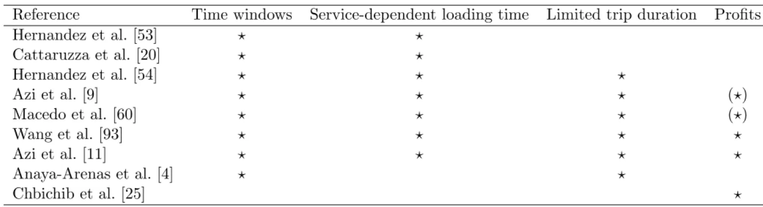
In this section, we are interested in a relatively limited number of papers and problems summarized in Table 2. We first describe the different extensions investigated and then discuss about mathematical formulations, available benchmark instances and solution methods. Detailed numerical results on all the instances tackled by the methods surveyed in this section are provided in Appendices B and C.

Reference Time windows Service-dependent loading time Limited trip duration Profits

Hernandez et al. [53] ? ? Cattaruzza et al. [20] ? ? Hernandez et al. [54] ? ? ? Azi et al. [9] ? ? ? (?) Macedo et al. [60] ? ? ? (?) Wang et al. [93] ? ? ? ? Azi et al. [11] ? ? ? ? Anaya-Arenas et al. [4] ? ? Chbichib et al. [25] ?

Table 2 – Main academic extensions of the MTVRP

Time windows (TW) indicates that with each customer i is associated a time interval [Ei, Li]

during which service should take place. Arriving at customer location earlier than Ei is allowed,

but makes the driver wait until the opening of the time window. On the opposite, late arrival is forbidden. The time horizon can then equivalently be represented by a time window [E0, L0] = [0, TH]

associated with the depot. When introducing time windows, authors generally also introduce service times Si at customers and a loading time S0 at the depot. Also, authors often introduce the notions

of travel cost or travel distance on arcs, both equal to Tij, in order to distinguish clearly between the

objective function and journey duration. The introduction of time windows has several important consequences. First, the duration of a trip is a function of the time at which it starts. Condition (iv) introduced when defining the MTVRP thus does not make sense anymore. Each trip is time-stamped in a solution and journeys are composed of trips that do not overlap. Furthermore local search becomes more complicated as modifications in a trip impact the rest of the journey. Secondly, solution schemes cannot exploit anymore a decomposition of the problem in two successive phase: a routing phase where trips are constructed and a packing phase where they are packed together to obtain journey. With time windows, trips cannot be properly evaluated as long as their starting time is not known and the construction of journeys is not anymore a question of packing but of scheduling. A simple illustration is given by the case where a single vehicle is available and the time horizon is large: while the MTVRP is equivalent to the VRP (with an unlimited fleet of vehicles), it is unlikely that a VRPTW solution can be transformed to its multi-trip counterpart.

Service-dependent loading times indicates that the loading time of a vehicle at the depot depends on the customers visited during the trip. All authors that consider service-dependent loading times consider a loading time proportional to the total service time of the trip. We note β the coefficient applied. A difficulty met with service-dependent loading times is the fact that any modification of a trip can influence the departure time of the vehicle from the depot (this is however not specific to the multi-trip situation).

Limited trip duration indicates that trip duration is limited by a value Tmax. For most authors,

the duration of a trip is the elapsed time between the departure time of the vehicle from the depot, after it has been loaded, and the moment the service starts at the last customer in the trip. These constraints are motivated by the fact that perishable goods must be delivered before a certain amount of time has passed from the moment they have been loaded. The only exception is Anaya-Arenas et al. [4] that address biomedical sample collection. The trip length is then the elapsed time between the arrival at the first customer of the trip and the arrival at the laboratory.

Profits indicates that serving all customers is not mandatory and a profit Pi is associated with

each customer i and represents the profit of serving customer i. In practice, the proposed instances consider equal profit customers and the objective function consists in minimizing the number of customers not served, breaking ties in favor of the minimum traveled distance. Parenthesis are added in Table 2 for Azi et al. [9] and Macedo et al. [60] because in their experiments all customers are visited most of the times; comparisons with Hernandez et al. [54] (that enforce the visit of all customers) are thus possible.

All these extensions are trivially N P-hard because they admit the MTVRP as a special case.

Mathematical formulations

Though no compact formulations have been proposed for the variants cited above, one can easily update the 4-index model introduced in Section 2 from other papers in the literature.

For time windows, we propose to add variables tvr

i defined as the time variables added in the

three-index formulation of the MTVRP proposed by Azi et al. [9]: tvr

i indicates the time at which

trip r of vehicle v visits customer i, if i is visited in the trip, 0 otherwise; tvr₀ indicates the starting time of trip r of vehicle v; tvr

N +1indicates its ending time. Time windows are then added by replacing

Constraints (5)-(6) with the following constraints:

tvr_i + Si+ Tij ≤ tvrj + M (1 − x vr ij) ∀i ∈ N , j ∈ N \ {0}, v ∈ V, r ∈ R, (65) tvr_i + Si+ Ti0≤ tvrN +1+ M (1 − x vr i0) ∀i ∈ N \ {0}, v ∈ V, r ∈ R, (66) tvr_{N +1}≤ tv,r+1₀ ∀v ∈ V, r ∈ R \ {N − 1}, (67) Eiyivr ≤ t vr i ≤ Liyvri ∀i ∈ N \ {0}, v ∈ V, r ∈ R, (68) tvr_{N +1}≤ TH ∀v ∈ V, r ∈ R, (69) tvr_i ≥ 0 ∀v ∈ V, r ∈ R, i ∈ N ∪ {N + 1}. (70) Constraints (65)-(67) compute time variables. Constraints (68) guarantee customer time windows. Constraints (69) impose that trips are finished before the end of the time horizon.

To take the service-dependent loading time into account, variables S₀vr are added, where S₀vr is the loading time for trip r of vehicle v. Constraints (65) are then changed to:

tvr_i + Si+ Tij ≤ tvrj + M (1 − x vr ij)∀i ∈ N \ {0}, j ∈ N \ {0}, v ∈ V, r ∈ R, (71) tvr₀ + S₀vr+ T0j ≤ tvrj + M (1 − x vr 0j)∀j ∈ N \ {0}, v ∈ V, r ∈ R, (72) and constraints S₀vr = β X i∈N \{0} Siyivr ∀v ∈ V, r ∈ R, (73) S₀vr ≥ 0 ∀v ∈ V, r ∈ R, (74) are added. Constraints (71)-(72) decompose constraints (65) to deal with the fact that the loading time at the depot becomes a variable. Constraints (73) compute this variable.

Limited trip duration is obtained adding:

tvr_i ≤ tvr

except for Anaya-Arenas et al. [4] where it is instead

tvr_{N +1}≤ tvr

i + Tmax ∀i ∈ N \ {0}, v ∈ V, r ∈ R. (76)

Finally, profits can be introduced by changing the objective function (1) to

max MP X i∈N \{0} X v∈V X r∈R Piyivr− X (i,j)∈A Tij X v∈V X r∈R xvr_ij (77)

and changing constraints (2) to

X

v∈V

X

r∈R

y_ivr ≤ 1 ∀i ∈ N \ {0}. (78)

where MP is a large constant that always makes beneficial increasing the profit, whatever the impact

on the traveled distance. Constraints (78) relax the obligation to visit customers.

Instances

Experiments in the above papers are all carried out on benchmark instances obtained from Solomon’s instances [82] and their extension proposed by Gehring and Homberger [45]. Solomon’s instances with small TW (groups R1, C1 and RC1) have however been excluded as, according to Azi et al. [9], they are not adapted to journeys with multiple trips. Following current practices for the VRPTW, smaller instances are generated by considering only the first customers.

Several parameters as the number of vehicles, the capacity of these vehicles or service times have been modified to increase the chance that vehicles perform multiple trips without obliterating the set of feasible solutions. For the case of service-dependent loading times, parameter β is always set to 0.2. For the case of limited trip duration, different values have been proposed for Tmax. For the case

of profits, profits are set to 1 for all customers. Customer locations in Gehring and Homberger [45] instances have been normalized in order to fit the 100×100 square as in Solomon instances.

Exact methods

Hernandez et al. [53] propose a branch-and-price algorithm for the MTVRP with time windows (MTVRPTW) and service-dependent loading times. They explain that the method developed by Mingozzi et al. [62] for the MTVRP cannot easily be extended because time windows strongly modify the structure of the problem. They investigate two formulations. In the first formulation, columns are journeys; in the second formulation column are trips (with a fixed schedule). The first formulation does not specially bring difficulties up, except for the size of the pricing problem solution space. The second formulation necessitates to solve a complex pricing problem, where column reduced cost depends on their timing. Note that in both cases the authors tackle the difficulty implied by service-dependent loading times by applying backward strategies when solving the pricing problems. Experiments show that the second formulation is more efficient. It is able to solve most instances with 25 customers (25 out of 27) and a few instances with 50 customers (5 out of 27). Values are reported in Appendix B, Table 4.

Several authors address the special case where trip duration is limited. This feature plus the presence of TW and the limited vehicle capacity that allows only few customers to be served in each trip, make the enumeration of all feasible trips achievable for small and medium size instances. The proposed exact methods are based on this observation. They all proceed in two phases. The first phase consists in listing all the candidate trips. The second phase aims at constructing the vehicle routes.

In the first phase, all authors apply the same method, based on labeling. Trips are constructed by extending labels from the depot in all feasible directions. Dominance rules are applied to delete trips that do not visit customers following the optimal sequence.

Three different methods are proposed for the second phase. In Azi et al. [9], an auxiliary graph is constructed, with a vertex and a TW for each trip. Arcs represent possible successions of trips. Phase 2 is then addressed as a VRPTW with profits and solved with a branch-and-price algorithm. In Macedo et al. [60], the second phase relies on a time-indexed graph. Nodes correspond to discrete time instants and arcs either correspond to waiting times at the depot or elapsed time during a given (time-stamped) trip. Phase 2 can then be addressed as a min-cost flow problem. In Hernandez et al. [54], a set covering formulation is proposed and solved with branch-and-price. Columns represent time-stamped trips. The pricing problem simply consists of finding a convenient starting time for trips.

In addition, Azi et al. [8] address the single vehicle case. They introduce the same auxiliary graph as in Azi et al. [9]. Because a single vehicle route is searched for, the problem they face is very similar to the pricing problem of Azi et al. [9]. They apply an equivalent dynamic programming procedure.

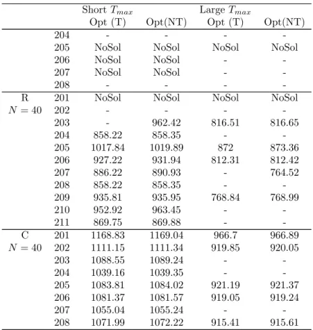
Experiments show that Macedo et al. [60] and Hernandez et al. [54] obtain comparable results and significantly improve upon Azi et al. [9]. The methods developed in Macedo et al. [60] and Azi et al. [9] are however more general as they solve the problem with the Profits feature described above. Optimal solutions are reported in Appendix C, Table 5 when all customers can be visited and Table 6 when the optimal solution only visits a subset of customers.

It can be observed from the results that, as expected, instances with short time limits and small feasible trip sets are easier to solve. Actually, one could note that none of the above approaches is specifically designed for problems with limited trip duration: they can be applied as soon as, and only when, the set of feasible trips is small.

Heuristics

We are not aware of any algorithm developed for the heuristic solution of the MTVRPTW. Cattaruzza et al. [20] however propose a population-based procedure for the more general MTVRPTW with Release Dates (see Section 3.5) and evaluate this procedure on the instances used by Hernandez et al. [53]. The principle of the algorithm is the same as in Cattaruzza et al. [21] (see Section 2), the main difference being the split procedure used for decoding chromosomes. In order to deal with time constraints, the assignment of trips to vehicles is managed within the split procedure, which turns out to search for a resource constrained shortest path. An adaptive heuristic dominance rule is introduced to limit computing times. All optimal solutions computed in Hernandez et al. [53] are obtained except one. Best known solutions are reported in Appendix B, Table 4.

When trip duration limits are added, we are aware of three papers. Anaya-Arenas et al. [4] propose two constructive heuristics completed by local search. The first heuristic creates trips and packs them into journeys. The second heuristic directly create journeys. Local search considers insertion of visits in later positions. The procedure is evaluated on a set of dedicated instances developed by the authors and based on real-world biomedical sample transportation. In both other papers, profits are considered. The first is from Azi et al. [11]. They propose an adaptive large neighborhood search. Destruction and insertion operators are developed for customers, trips and journeys. The second is by Wang et al. [93]. They propose an algorithm based on the Adaptive Memory Procedure paradigm. Each solution that is constructed is inserted in a memory M. When M reaches a certain size, a solution is constructed selecting trips randomly with a distribution based on the quality of the solution they belong to. Results obtained by Wang et al. [93] outperform those provided by Azi et al. [11] with respect to quality, but the procedure is on average three time more expensive in terms of CPU time.

Chbichib et al. [25] consider the MTVRP with profits but without TW nor limited trip duration. A two-phase algorithm is designed. Solution construction is guided by the net profit : next inserted customers maximize the difference between the profit and the extra routing cost needed to serve the customer. Improvement is carried out with a variable neighborhood descent algorithm and a hill climbing procedure. Both are based on swap, insertion and cross-exchange moves.

3.2

Production, inventory, routing problems

Many times, vehicle routing optimization is only a step in a more complex decision-making process involving also production and inventory management. Traditionally, these problems are decoupled and optimized separately. There are however several reasons that can motivate to address them simultaneously. Firstly, because of strong temporal constraints, it might be necessary to synchronize the different types of operations (production and transport). Secondly, a coordinated optimization can often allow reaching a better global efficiency. Recently, these issues have received a lot of attention in the literature. It resulted in the publication of several survey papers (Chen [26], Coelho et al. [32], Bertazzi et al. [14], Adulyasak et al. [1]). In this large amount of literature, a few papers allow multiple routes in the routing phase. We focus on these papers below. We organize the section by splitting them in three subgroups: production-routing, inventory-routing, production-inventory-routing.

Synchronization between production and routing is particularly important in make-to-order poli-cies where customized products are produced and delivered to clients within short time. No (or almost not) inventory is considered and then addressing simultaneously production and transportation is cru-cial. In the context of newspaper production and distribution, Van Buer at al. [92] explain that (daily overnight) distribution starts long before the production is finished, vehicle routes are relatively short and it is important to organize journeys with successive trips to satisfy drop-off time windows with a limited fleet of vehicles. Ullrich [91] considers an academic but practice-oriented production-routing problem with similar characteristics. Lee et al. [56] address the integrated production-distribution of radioisotopes for medical treatments. Because of the very short lifespan of this medicine, distribution with multiple trips is required. Besides, due to the natural decrease of radiation levels, the quantities produced depend on the delivery times. Geismar et al. [46] finally consider the distribution of an adhesive of limited lifespan with a single vehicle. In their case, production is performed at a fixed production rate and the successive trips of the vehicle have to be scheduled in accordance with the product availability. A few other papers also consider multiple trips, but with very small routes (one or two customers, e.g., Chang and Lee [24]), which falls beyond the scope of this survey. In all the aforementioned papers, solution methods concentrate on the complex synchronization between production and routing and are not specifically innovative in the way multiple trips are handled. The only exception can be found in Lee et al. [56] that give a polynomial time procedure to assign a set of time-stamped trips to a minimum number of vehicles.

Aghezzaf et al. [2] introduce the possibility of multiple trips in inventory routing. In this class of problems, a set of customers consumes a product at a certain rate; the supplier needs to determine, over a time horizon of several periods, when to visit customers, which quantity to deliver at each visit and how to organize routes. By allowing multiple trips in routes, Aghezzaf et al. [2] permit to replenish with a vehicle a set of customers whose demand is larger than the vehicle capacity. Higher delivery quantities are then possible at the cost of traveling additional distance to reload the vehicle at the depot. The authors show how it impacts the economic order quantities and eventually decreases total inventory holding costs and ordering costs. Raa and Aghezzaf [75] and Raa and Aghezzaf [74] pursue this line of research, but limiting the driving time per period and giving the possibility of assigning different frequencies to the trips of a vehicle, respectively. Solution approaches in the three papers are based on an equivalent heuristic column generation procedure where new columns are obtained with a modified savings algorithm. In this algorithm, the savings

obtained when joining two vehicle journeys is computed by evaluating the savings (and feasibility) for all possible combinations of ending trip for the first journey and starting trip for the second.

Cornillier, et al. [33] address inventory routing in the context of petrol station replenishment. Vehicles are allowed to perform several trips during each period. Several side constraints are present: the fleet of vehicles is heterogeneous, vehicles have different compartments, trip duration is limited, among others. A multi-phase heuristic is proposed. Trips are first constructed for each period and then packed into vehicles. Cornillier et al. [36] extend this work to the case of time windows.

Oppen and Løkketangen [68] and Oppen et al. [69] study a livestock collection problem that deals with transportation of live animals from farmers to slaughterhouses. Inventory constraints are imposed at the slaughterhouse: on one side, non-working periods should be avoided, on the other side animals cannot spend more than one overnight at the slaughterhouse. Rules to secure animal welfare are considered: mixing animals of different types in the same vehicle compartment is not allowed; animals with and without horns cannot be mixed; herds that are infected should be collected as the last of the trip. The fleet of vehicles is heterogeneous. A tabu search and a column generation approach are proposed.

Finally, Lei et al. [57] seek to optimize conjointly production, inventory and distribution in the chemical industry. The problem involves several production sites, each one with its own fleet, and vehicles are allowed to perform several delivery trips at each period. The authors propose a two-phase approach. In the first phase, a mixed-integer program is solved where vehicles are allowed to serve customers only via direct shipment. In a second phase shipments are heuristically consolidated.

3.3

Multi-trip in maritime transportation

Vehicle routing problems have mainly been developed in relationship with the transportation of goods or passengers on road networks. Models used for vessel route optimization however share obvious similarities with the VRP: optimized sequences of port visits where cargoes are picked-up and/or delivered are searched for. There are however important differences that we list below, before moving to MTVRP-related papers. Readers interested in maritime transportation are referred to Christiansen et al. [28] and Christiansen et al. [27].

First of all, the usual goal in maritime transportation problems is to minimize sailing costs and time charter costs, i.e., costs due to the rent of vessels. Classical vehicle routing problems usually focus on minimizing travel costs; when vehicle costs are considered, because the fleet needs to be sized, it is simply modeled with fixed costs. Conversely, the integration of charter costs can be more tricky. Second, in maritime transportation the size of vessels is generally critical: different sizes of vessels are usually available, with different renting costs and characteristics (capacity, sailing speed, accessibility to ports, etc.). Classical vehicle routing problems usually consider a homogeneous fleet. Other differences are the length of the time horizon TH that goes from a working day in standard

vehicle routing problems to weeks in the maritime case; truck routing times are shorter than vessel sailing times; problem sizes are generally bigger in land transportation than in maritime. Another remarkable difference is that usually the notion of depot is absent in maritime problems.

There are however a few practical situations that fall into the multi-trip definition we gave in Section 1. We identified two: the supply of offshore platforms from an onshore depot and short-haul hub-and-spoke feedering.

Fagerholt [41] investigates a liner shipping problem (LSP) in order to find a set of vessels and an order of visits to offshore platforms to minimize sailing and charter costs respecting capacity and time constraints. Vessels are allowed to be re-sailed once they are back at the onshore supply depot. The author proposes a three-phase method to solve the problem. First, for each type of vessel, all the feasible trips are generated. Second they are packed together into feasible journeys. The largest size vessel associated with trips forming the journey is associated to the journey itself. Third, a set partitioning problem is formed on the set of trips and journeys determined in phase one and two.

A real instance formed by 15 nodes and 5 different vessels available is solved. Moreover, three test instances with 20, 30 and 40 customers are evaluated.

Suprayogi et al. [83] adapt this algorithm for the case when port’s water depth is taken into account and ships cannot have access to all ports. The study is motivated by oily liquid waste collection from ports in the Indonesian territory.

Fagerholt and Lindstad [42] extend the work initiated in [41] by introducing temporal aspects. Some offshore platforms close overnight, generating a time window for service. The algorithm pro-posed follows the same scheme: first, all the feasible trips are generated, then a solution is constructed solving an integer programming model.

Halvorsen-Weare et al. [52] pursue this line of research with a much more complicated problem. Offshore platforms require several visits during the time horizon. Departures from the onshore supply depot to the same offshore platform need to be evenly spread. Onshore and offshore platforms are constrained by opening hours. Finally trips need to be neither too short (for better capacity exploita-tion) nor too long (sailing times uncertainty increases in long time periods). Again, Halvorsen-Weare et al. [52] adapt the scheme initially proposed in Fagerholt [41]. Instances with up to 14 offshore platforms are considered. Visits to platforms vary between 1 and 6 during the time horizon. Shyshou et al. [81] address the same problem with a large neighborhood search. An interesting issue deserves to be underlined here. The problem can somewhat be classified in between the classes of multi-trip and periodic problems. It is not a standard periodic problem (which would fall out of the scope of this survey) because journeys can cover several periods. However, contrary to usual multi-trip problems, time is discretized in the sense that a vessel is not allowed to finish and start a trip on the same day. Improving the duration of a trip by a few hours can thus sometimes save a whole day. This is all the more important in this context given that the main objective of the problem (and the main strategy of the local search procedure) is to limit the number of vessels used.

Bendall and Stent [13] are concerned with short-haul hub-and-spoke feedering. They investigate the profitability of fast cargo services, where a great number of round voyages can be achieved quickly. In their model, ships start from the container terminal and can visit any number of times each port. The objective is to maximize the revenue earned from transported containers minus shipping costs. The solution method starts by computing a set of possible trips. A mathematical model is then solved in order to determine how many times each trip is performed (possibly zero). Trips are finally heuristically packed into journeys. A simple case study based on South East Asia is given as an example.

3.4

Multi-level distribution with multi-trips

Another category of problems involving multiple trips can be found in the context of multi-level distribution. The main peculiarity in these problems concerning the multi-trip aspect is the presence of multiple depots. Contrary to the common practice for the multi-depot VRP, the fact that vehicles can perform multiple trips leaves the possibility that a trip starting at a depot ends at another depot. The literature on the multi-depot VRP has largely been influenced by the possibility of a two-phase strategy: first assign customers to a depot, then optimize routes for this depot. With the new option offered when multiple trips are allowed, algorithms based on this strategy are dismissed and the movements of the vehicles planned from the different depots are much more deeply interlinked.

Examples of papers dealing with this issue are Crainic et al. [37], Nguyen et al. [64], Nguyen et al. [65] and Grangier et al. [48]. All these papers address multi-level distribution for city logistics. Delivery flows are organized as follows. Direct delivery to customer is forbidden. Goods are first delivered to satellites by first-tier vehicles, from where they are loaded in small-capacity vehicles (second-tier vehicles) for final delivery to customers. No storage is allowed at the satellites. A journey of the second-tier vehicles typically starts from (and ends at) a central depot and is constituted of several successive trips, each possibly starting and ending at different satellites.

In Crainic et al. [37], Nguyen et al. [64] or Nguyen et al. [65], second tier-vehicles have to reach satellites during very restrictive time windows, derived from the arrival times of first-tier vehicles. Thanks to these time windows, the optimization of the trips can almost be decoupled. This is the approach proposed in Crainic et al. [37]. They first compute vehicle trips for the different satellites and then constitute journeys by solving a minimum cost network flow problem. As shown in Nguyen et al. [64], the weakness of this approach is to badly intertwine the routing and the satellite assignments. Nguyen et al. [64] propose instead a tabu search approach. In addition to standard routing moves, relocation and exchange of trips between vehicles are introduced. Nguyen et al. [65] extend the algorithm to a more complex problem involving both inbound and outbound flows.

Grangier et al. [48] optimize simultaneously the first-tier and two-tier fleets of vehicles. They thus have to manage the synchronization of the two types of vehicles at the satellites. They tackle the problem with an adaptive large neighborhood search heuristic. The focus is then more on the synchronization between the two fleet of vehicles than on the synchronization between the successive trips of second-tier vehicle.

Plenty of more distant problems where a relatively similar situation is found are treated in the literature. Illustrative examples are given by the multi-depot VRP with inter depot routes (Crevier et al. [38]) or other papers dealing with intermediate facilities for recharge and refill (see Gianessi [47] for a recent survey). Reviewing in details this paper is out of the scope of this survey.

3.5

Other variants of the MTVRP

Many other variants of the MTVRP have been studied in the literature. We propose in this subsection to elaborate on the characteristics of the problems that interfere the most with the multiple trip component. We then explain how the challenges raised by these characteristics have been dealt with.

Original temporal constraints

Several original temporal constraints have emerged in the context of VRP with multiple trips. A first noteworthy constraint is the so-called double time window for the depot considered in Hajri-Gabouj and Darmoul [51]. In general, the time window associated with the depot is defined by two parameters: an opening time, before which vehicles are not allowed to start, and a closing time, before which vehicles must have finished their journey at the depot. Hajri-Gabouj and Darmoul [51] introduce a third parameter: the latest time at which a vehicle is allowed to start one of its trips from the depot. This new constraint is motivated by the fact that facilities used for loading the vehicles can be closed earlier than the depot. Though the constraint sounds important practically, its impact on solution methods seems rather limited (a genetic algorithm in the case of Hajri-Gabouj and Darmoul [51]).

Battarra et al. [12] impose the duration of the journey (difference between the instant the vehicle is back at the depot after performing the last trip and the instant at which loading operations of the first trip start) not to be longer than the spread time ST. The spread time differs from the time

horizon TH and it is usually strictly shorter (the spread time becomes meaningless when it coincides

with the time horizon). The spread time models the driver working day length, when this is shorter than the depot opening hours. A vehicle starting its journey before TH − ST (assuming the depot

opens at time 0) must not take longer than the spread time; while on the other case must be back at the depot before the time horizon is over. Battarra et al. [12] solve the problem with an adaptive guidance approach that penalises the creation of trips that heavily overlap on certain time intervals. This is to favour trip packing into journeys.

Cattaruzza et al. [20] introduce so-called release dates. A release date represents the time at which goods are available at the depot for the final delivery to a customer. Note that commodities are not transferable between customers. It is motivated by distribution from mutualized platforms:

given a customer request, goods are first supplied by trucks in the platform at the time of the release date, and are then available for final distribution (with eco-friendly vans). These constraints raise the difficulty of finding a balance between starting trips early to optimize the use of the vehicles and waiting at the depot to reach a more effective consolidation of the merchandises. The authors address the MTVRPTW with Release Dates with the genetic algorithm described in Section 3.1. They explain how the split procedure and local search moves can be adapted when release dates are introduced.

Mu and Eglese [63] study a relatively similar situation except that a single commodity is involved. Part of the commodity that has to be delivered is supposed to arrive late at the depot (the time and the quantity are known). This simulates the disruption of one of the vehicles in charge of delivering the merchandise to the depot. The objective is then to minimize a weighted sum of service delay, drivers overtime, and the deviation from the original plan that is calculated supposing all the merchandise available at the beginning of the day. Vehicles are allowed to wait at the depot until the late merchandise arrives or can leave the depot for a first delivering trip and possibly perform a second trip when they are back. Note that journeys are made by not more than two trips: one that starts before the late arrival of merchandise and one that starts after. The problem is called Disrupted Capacitated Vehicle Routing Problem with Order Release Delay and is solved by means of a tabu search algorithm.

Another situation investigated in Azi et al. [10] is the dynamic setting where new requests arrive during the day. New requests can then either be rejected or be integrated in future trips of the vehicles.

Distribution of incompatible products

Another interesting situation is found when multiple incompatible commodities are transported (Bat-tarra et al. [12], Cattaruzza et al. [22]). The context is the distribution of different types of products to supermarkets located in a regional territory. Commodities are said incompatible because they cannot be transported together in a vehicle. If multiple trips were not allowed, each vehicle could be assigned to a commodity and the distribution problem would naturally decomposes in one routing problem per commodity. On the contrary, in Battarra et al. [12] and Cattaruzza et al. [22], vehicles can perform several trips; hence, the different trips of the journey of a vehicle can be devoted to the distribution of different commodities. This possibility strengthens the connection between the different commodities and complicates the problem. The definition of the problem considers a fixed maneuvering time between each pair of successive trips in addition to loading times that depend on the quantity transported in the trip. The maneuvering time can be seen as the time needed to prepare the vehicle for the next trip and can include cleaning operations when service switches to a different commodity.

Limited number of trips

An easier type of constraint explored in the literature is the limitation of the number of trips allowed in the journeys (Povlovitsch and Bergsten Mendes [71], Alonso et al. [3], Gribkovskaia et al. [49]).

As seen in Section 2.1, a positive consequence of this constraint can be a tighter integer pro-gramming formulation for the problem. Indeed, considering for example the 4-index formulation, less values are needed for the index on the number of trips and less variables are involved in the formulation.

Fleet size minimization an other objectives

In several references (Prins [72], Battarra et al. [12], Cattaruzza et al. [22]) the objective of minimizing the fleet size is introduced. Considering a limited fleet of vehicles or trying to minimize this fleet