All-optical method of nanoscale magnetometry for ensembles of nitrogen-vacancy defects in diamond

All-Optical Method of Nanoscale Magnetometry for

Ensembles of Nitrogen-Vacancy Defects in Diamond

by

Nicolas A. Lopez

Submitted to the Department of Nuclear Science and Engineering

in partial fulfillment of the requirements for the degree of

Bachelor of Science in Nuclear Science and Engineering

at the

MASSACHUSETTS INSTITUTE OF TECHNOLOGY

June 2015

MASSACHUSES INSTITUTE

@Nicolas

Lopez, 2015. All Rights Reserved.

MAY 12016

LIBRARIES

Author...Signature

redacted

Department of Nuclear Science and Engineering

May 8, 2015

Certified by...Signature

redacted

Paola Cappellaro

Esther and Harold E. Edgerton Associate Professor

of Nuclear Science and Engineering

Thesis Supervisor

',?A [12

Acceped bySignature

redacted

A ccepted by ... . . . . .. a. .r ....e . .. .

Michael Short

Assistant Professor of Nuclear Science abd Engineering

Chair, NSE Committee for Undergraduate Students

AUthor hereby grants to Mi p"1h80 ft sprodw _{and to}

*bue _{publicly paper and delsvnl copies of this thesis dseutm} b wioe

All-Optical Method of Nanoscale Magnetometry for

Ensembles of Nitrogen-Vacancy Defects in Diamond

by

Nicolas A. Lopez

Submitted to the Department of Nuclear Science and Engineering on May 8, 2015, in partial fulfillment of the

requirements for the degree of

Bachelor of Science in Nuclear Science and Engineering

Abstract

The Nitrogen-Vacancy (NV) defect in diamond has shown considerable promise in the field of small scale magnetometry due to its high localization and retention of fa-vorable optical properties at ambient conditions. Current methods of magnetometry with the NV center achieve high sensitivity to fields aligned with the defect axis; how-ever, with most present methods transverse fields are not directly measurable. The all-optical method of NV magnetometry provides a means to detect transverse fields by monitoring changes in the overall fluorescence profile. In this work the all-optical method is extended to ensembles of non-interacting NV centers. By establishing an external bias field aligned with the (1, 1, 1) axis, the magnitude of an unknown trans-verse field can be unambiguously identified through the measurement of the signal curvature. The angular orientation can be determined up to a two-fold degeneracy by observing the change in signal curvature produced when the bias field is shifted off-axis. The magnetometry method explored in this thesis thus provides good sensi-tivity to transverse fields, while reducing to a minimum the experimental apparatus required to operate the magnetometer.

Thesis Supervisor: Paola Cappellaro

Title: Esther and Harold E. Edgerton Associate Professor of Nuclear Science and Engineering

Acknowledgments

I would like to thank Professor Paola Cappellaro for her continued support and assis-tance throughout the duration of this project. I value the insight and intuition gained through our many discussions about the NV center and its fascinating dynamics and applications, of all of which I had no prior knowledge when beginning this project.

I am especially grateful for the numerous comments and suggestions she provided to me as I worked to develop the incoherent and unorganized scribbles of my own notes into a comprehensible text. Much of the clarity in this paper is due to her detailed feedback.

Contents

1 Introduction 15

2 Background 17

2.1 Background . . . . 17

2.1.1 Spin Structure of the Nitrogen-Vacancy Defect . . . . 17

2.1.2 Detection of Magnetic Fields with the

N V Center . . . . 18 2.1.3 All-Optical NV Magnetometry . . . . 20

2.1.4 Non-degenerate Time-Independent Perturbation Theory . . . 21

2.1.5 The Seven-Level Model of the NV Spin Level Structure . . . . 22

3 Model Details 25

3.0.6 Calculation of ij3 via Non-degenerate TIPT . . . . 26

3.0.7 Numerical Details of the Transition Rates . . . . 28 3.0.8 Reformulation of the Model Equations as a Linear Matrix System 29 3.0.9 Extension to Ensembles . . . . 31

4 Detection of Magnetic Fields 37

4.0.10 Parallel Fields . . . . 37 4.0.11 Transverse Fields . . . . 41

5 Conclusion 51

A Approximate Nullspace of M 55

List of Figures

2-1 The seven level model in the absence of an external magnetic field, con-sisting of the ground state and excited state triplets and a metastable singlet. Only spin-conserving radiative transitions and non-radiative transitions to the metastable state are considered. . . . . 18 2-2 A depiction of the Zeeman splitting of the triplet ground state. ... 19 2-3 The normalized PL intensity as a function of the transverse magnetic

field amplitude. The parallel projection onto the defect axis is held constant at B, = .03T. . . . . 21

3-1 (Left) The tetrahedral geometry to be considered. The tetrahedral

angle is 109.5' and p is the angle between B and z. (Right) The tetrahedral geometry projected into the transverse plane. The angle of symmetry is 1200 and

#

is the offset of the tetrahedron with the x-axis, which is defined along the transverse field component. . . . . 32 3-2 Rotation profiles of the observed signal within the x-y plane. p, the

angle between B and 2, increases from top to bottom from 20' to 85' to 90'. For all, BI= .03T and F is set to 10. The intensities are

normalized to the p = 0' intensities. . . . . 34 3-3 A full 47r rotation map of the NV tetrahedron. p is the polar angle of

the external magnetic field and

#

is the azimuthal angle. JBI is .M1T and F is set to 10. . . . . 35

4-1 A demonstration of the increased sensitivity of the NV center to

per-turbing transverse fields around the LAC regions - .05T and .1T. On the left is the single NV case, while on the right the full ensem-ble is considered. Circled are the 3 symmetry points about which a perturbing parallel field could be readily identified with the methods discussed in the text. F = 10 in both cases. The small deviations that occur near the LAC points are due to divergences in the coefficients coj that develop as a manifestation of the Perturbation Theory and are not physical. . . . . 38

4-2 The geometry of the perturbing magnetic field. T is the angle between the perturbing field and the z-axis, and Q is the angle between the perturbing field and the x-axis. . . . . 41

4-3 A plot demonstrating the effect of the transverse field on the observed signal when the system is biased around the excited state LAC. Clearly the observed signal approaches a steady value for B, > .002T. In generating this plot B, = .05T and F = 10. . . . . 42

4-4 A series of plots depicting the dependencies of the signal curvature on B, (Top), / (Middle) and F (Bottom). Clearly, a change in the transverse field magnitude is the dominant cause for changes in the observed signal curvature. It is therefore proposed that by monitoring the changes in the signal curvature the transverse perturbation mag-nitude can be determined. . . . . 43

4-5 (Blue) A plot of the curvature of the signal profile evaluated at B2 = .052T and F = 10 as a function of B,. (Green) A fitted curve -=

.052

58038 ;2 to extract the leading order dependence of the signal

4-6 The rotational symmetry of the total transverse field (red). The dot-ted circle represents the projections of equal B1 and is what would be observed experimentally. For a fixed transverse bias field B (black), any transverse perturbing field b1 (blue) that creates a B1 with the

observed magnitude is an allowable solution due to the rotational in-variance of the signal curvature. For the case lal > 1 there is one positive solution for b1 for all values of Q in the range [0, 27r]. For the case

|a|

= 1 there is one positive solution for b1 for all values of Q in the range

[E,

].

For the case lal < 1 there are only positive solutions for b1 for the negative angle interval when I sin QI

<

Ial. Usually there are 2 possible solutions on this interval, but when Isin

QI

= IaI there is only one tangent solution. . . . . 47

List of Tables

3.1 The rate values used in the calculations presented in this thesis. All transition rates not shown are taken to be 0. . . . . 29 3.2 The parallel and perpendicular projections of an external magnetic

field B = BXJ + Bs onto the 4 possible defect axes. The angles 0,

#

and <po are defined in the text. . . . . 32

Chapter 1

Introduction

The accurate measurement of magnetic fields at small scales can be beneficial for a variety of scientific endeavors. For example, measuring with high spatial resolution the magnetic field produced by nuclear spins of a protein can yield information re-garding its molecular structure

[1-3],

and dynamic imaging can reveal the manner in which proteins fold and unfold

[4-8].

Furthermore, intracellular processes and mechanisms can be better studied by monitoring the distribution and evolution of magnetic moments within the cell

[9-141,

with better spatial resolution yielding bet-ter understanding. Currently used methods of small scale magnetometry, including superconducting quantum interference devices [15-17], atomic vapor based magne-tometry

[18,

19], and magnetic resonance force microscopy [20-221, are either not capable of resolving changes on a nanometer scale, or require special operating condi-tions, such cryogenic temperatures or large sample sizes, which are technically chal-lenging and not suitable in certain contexts. Thus for high precision measurements that are to be performed in ambient conditions, a new method of magnetometry is necessary.

A suitable candidate is the Nitrogen-Vacancy defect in diamond, which promises nanoscale precision even when operated at room temperature

[23-25].

A NV center occurs when a nitrogen substitutional defect is located next to a vacancy in the lattice structure, which can occur naturally or can be induced through laboratory

methods [26-30]. Of interest to this project is the NV- center1, in which an additional

electron is located within the defect site.

The NV center is known as a color center because it fluoresces within the visible spectrum when optically excited. As will be discussed in more detail, the intensity of the emitted light is intimately related to the spin state of the NV center, and because quantum spins interact with magnetic fields in a well-understood manner, by monitoring changes in the intensity of the NV center fluorescence emission, the local magnetic field profile can be reconstructed.

In this work, we quantitatively analyze a method of NV magnetometry known as the all-optical method [31, 32], both analytically and numerically, and ultimately extend this model to include the effect of ensembles of NV centers rather than a single defect center. In Section II we introduce the relevant features of the NV center that make all-optical magnetometry possible. In particular, we introduce the effects of magnetic fields on the NV spin states, via the Zeeman effect, and introduce the optical rate equation model. In Section III we develop the model equations in more detail and modify them to be more convenient for computational analysis. Finally, section IV presents the results of the solved model equations and discusses the implications of the results on future experimental implementations of the all-optical method of NV magnetometry.

Chapter 2

Background

2.1

Background

2.1.1

Spin Structure of the Nitrogen-Vacancy Defect

The ground state of the NV defect is a spin-I triplet. There is a zero-field splitting of the triplet state of Dgs = 2.87 GHz due to spin-spin interactions that places the 10) state below the 1

)

states. This triplet ground state can be excited with 532 nm wavelength laser light into an excited triplet state with D,, = 1.42 GHz zero-field splitting1. The subsequent relaxation process will yield an amount of photons dependent upon the relaxation path.

The dominant mode of relaxation is through spin-conserving transitions

[33,34];

for example, a state belonging to the excited state manifold will transition to its equivalent spin state in the ground state manifold, emitting a photon in the process to satisfy overall energy conservation. However, the total number of photons emitted after repeated optical stimulations is highly dependent upon the initial polarization of the state [35,361. This is due to the finite probability that the 1t) states will transition to the 10) state via a metastable singlet state2_{, a process known as intersystem crossing}

'It is the preservation of this unique spin level structure at room temperatures that allows NV magnetometry to be operable in ambient conditions

2

Note: the opposite phenomenon, the excited 10) state transitioning to a 1 ) state via the metastable state, is negligible compared to the probability of radiative decay.

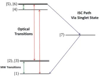
14)

ISC Path Via Singlet State

Optical

Transitions ₇

12),13)

MW Transitions

I1)

Figure 2-1: The seven level iodel in the absence of an external magnetic field. con-sisting of the ground state and excited state triplets and a inetastable singlet. Only spin-conserving radiative transitions and llon-raldiative transitiolns to the Ietasta)le state are considered.

(ISC). This transition excites phollonIs ill place of photon1s. so on average the observed number of, photolls ellitted bly the l ) states is less than that of the 10) state. Fig. 2- 1

gives a visual representation of the electronic and spin level structure of the NV defect.

2.1.2

Detection of Magnetic Fields with the

NV Center

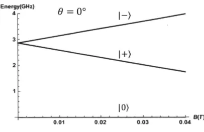
Spins interact with external magnetic fields through what is known as the Zeeman Effect. where spins alignled with the magnetic field will occupy a lower energy state than spins anti-aligneld to it. In particular for the spin- 1 triplet state of the NV defect and a magnetic field aligned with the defect axis, the energy of the 1+) state is shifted

downward by the amount pqB ~ (0.1.16 meV T) -B. the energy of the |-) is shifted upward by the same amount and the energy of the 10) state is unaffected, as can be seen inl Fig. 2 - 2.

Experimentally. this splitting cal be observed by performing microwave (MW)

Energy(GHz)

0.01 002 0.03 0.04

Figure 2-2: A dlepiction of' the Zeemiani splitting of' the triplet, grouind state.

the MW\ i's resonanit with the 10) --- ) transition at tI he applliedl mnagnietic field 1371.381. Monitoring the elet in~ resomniie (ESR ) spectra of' the NV cenlter provides a

mietlhod of extracting the mnaginitude of the external magnletic field pro jectedl onto the

defect axis (Ilie( to the known relation b)etweein the energy sp~litting andI thle external

linagnetic field: however, this (detection miethodl is in1sensitive to t ranisverse fields.

Similarly, another NV magietonietivinetlio( is the use of a Ramsey-type pulse s(jlIeiice- fo)r DC fields and~ Spin-echo measurements for AC fields 13 421. These

niethods conisists of' a resonian t MWNN pullse followedl by a period of* tree evohitioii InI

2

wvinch the ) states will pjick il) a Iphiase duel( to their interaction with the external

iagnectic field. followved bya fnal NR pu ~llse which p)rojects the s"tate b~ack onto

22

the original axis. This final pulse Zrnslates the phase iflerence obtaine (luring the periodl of free evolution (which is proportional to the magnetic field) to

a niasirahle (ifference in spin state Eopulations. An additio al pulse is Iserted in the id ale of the echo sequence 14f1 that will "flip" the state afi nd the direction of the spin evolution, allowing the phase (liflereince to continue to increase eveil as the external field magnetic field chnges sign. while canceliig (t, the (-flet s of static.

iagnetic noise, such as that arising fom a spin bath eiiviroiiiieit sp.

Whil these tecliliques cikn achieve good seisitivity, they are also insensitive to

trnsvhersdl f'tehosqe

[3

ht wl"fi"te stiat lvdrive thresiln

transitions via MW fields. Therefore, a third method of NV magnetometry, known as the all-optical method, is now introduced that is capable of directly detecting the presence of a transverse magnetic field and considerably simplifies the experimental apparatus since it only requires laser excitation and light detection.

2.1.3

All-Optical NV Magnetometry

In the absence of continuous or pulsed MW driving, an aligned magnetic field will cause no changes in the photoluminescence (PL) intensity as its magnitude is varied; the same, however, is not true for transverse fields. In strong transverse fields, the

mS basis with respect to the spin axis is not a good eigenbasis in which to analyze

the system; instead, an eigenbasis with respect to the axis of the magnetic field would serve better [44]. Eigenstates in this new basis can be expressed as superpositions of the previous m, states and as a consequence there will be a nonzero overlap between the 10) in the new basis and the ims = ) of the old basis. Through this effect, the contrast in photons emitted by the 10) and the 1 ) states is reduced; however the net intensity of the photon light is also reduced due to the larger population of

+

) states (see Fig. 2 - 3). While this behavior is intuitive for the case of a strong transverse field, this reduction in PL intensity will occur even in the regime of small transverse fields as long as the transverse field is nonzero. It may therefore be possible to detect the presence of transverse fields by monitoring a change in the intensity of emitted light.

For a single NV center, this approach is strictly limited to the detection of trans-verse fields. However for ensembles of NV centers this limitation is removed. The diamond lattice has a face-centered cubic structure; correspondingly, there are four possible spatial orientations for the NV defect [45]. An external magnetic field par-allel to one NV center will be at an angle with the symmetry axis of another NV center within the sample. Therefore, when considering ensembles of NV centers, the all-optical method of magnetometry can be used to detect magnetic fields of any orientation.

mea -Normalized Intensity 1.0 0.8 0.6 0.4-0.000 0.002 0.004 0.006 0.008 0.010

Figure 2-3: The normalized PL Intensity as a function of the transverse magnetic field amplit ude. The parallel projection onto the defect axis is held const ant at B. - .03T.

snremiienits of a small magnetic field; however. with the increased sensitivity coies an expected decrease in simplicity of experimental (esignl. The imethods developed

ill this thesis project aim to accomplish the opposite: a relatively quick and simple method of detecting simmall iiiagmietic fields at the expense of decreased precision in the

measurement. The results of this project caii le uised to develop a tool for performing fast measurements when the ultimate sensitivity is hot the primary concern (although

nanoscale spatial resolution is still obtainable, even with such aii "imprecise" device). or an apparatus that cali be lised ill tabletop demonstrations in either laboratory

settings or a presentation to a general audience, since the ineasuremnent methods will

be simple to perforum.

2.1.4

Non-degenerate Time-Independent Perturbation Theory

Perturbative anialysis is useful for systems in which small changes are made to an exact ly-solva ble unperturbed Hamiltonian, as is the case with the interaction of ai

external magnetic field with the NV defect. The total eigenstates and eigenvalies are then expanded in a power series around the small perturbation and truncated at ali appropriate order. That is to say., w(' 1)egin with an muperturbed Hamiltonian Ho

withii uiuhperturbed eigenstates 11()) such that

A small perturbation is added to the original Hamiltonian such that

Htot = Ho + 6H (2.2)

where 6H is small compared to Ho. The eigenvalues are then modified according to the equation:

I (m0| 6H |no) |2

E,= E, + n6H I no) + EO- E +.. (2.3)

m: n n m

Similarly, the eigenstates will change according to the equation:

In) = In

)

+ E E 6H E ) ... (2.4)

mon n

These results will be used in the next section to calculate the Zeeman interaction for the NV defect.

2.1.5

The Seven-Level Model of the NV Spin Level Structure

The NV system can be described by a seven-level model that comprises the electronic spin triplets in the ground and first excited state, as well as a singlet metastable level. The zero field eigenstates

{

i)} form a complete basis. Therefore, the new eigenstates

that result from the application of the external magnetic field (denoted as ji)') can be expressed as a linear combination of the original states [31]:

7

-i)

=

Z

ic (B) Ij)

(2.5)

j=1

where the coefficients aij(B) will be determined via Perturbation Theory (PT) in the following section and are functions of the external magnetic field. To describe the optical processes, we would need to work in an extended Hilbert space to analyze the time-evolution of the 7 x 7 density operator. However, only the diagonal elements of the density matrix are non-negligible and thus we can reduce the complex evolution

to rate equations for the seven population levels.

Transition rates are represented as kij for the transition from the i-th population level to the j-th population level. In a similar manner to Eq. 2.5, the new relaxation rates (denoted as k' ) will evolve as combinations of the zero-field transition rates 131]:

7

kij= I

C ajq|2_{kpq (2.6)}

p,q=1

The time evolution of the spin state populations can be well approximated with the classical rate equations [311:

dn

dt=Y k ,r - k 3mi (2.7)

j=A

However, for the purposes of the all-optical measurement approach, the above equation will be solved in the steady-state condition, with -- _dt -+ 0. Physically, this

corresponds to an experimental setup in which the NV center is optically excited long enough for transient behavior to diminish, and then photon collection will occur

while the NV center is continuously illuminated such that the steady-state condition

is maintained for the entirety of the measurement period. Thus, the equation to be solved is:

7

0 = k - k hi (2.8)

i,j=1A

where the spin state populations are denoted as hi to indicate they are the steady-state populations. The spin populations represent the probabilities for a single NV center to be in the specified spin state, thus the following normalization condition is

imposed on {ni} [31]:

7

1 (2.9)

Recall that the decay of the excited state manifold to the ground state manifold via the metastable state excites phonon production rather than photon emission, thus the only radiative decays are those from the excited state manifold directly to the

ground state manifold. Thus the rate of total radiative decay, R, is defined with the following equation 131]:

6 3

R = E k hi (2.10)

i=4 j=1

Chapter 3

Model Details

In the seven-level model the complete Hilbert space will be decomposed into 3 in-dependent subspaces - the ground state manifold, with the basis

{1)

, 12), 3)}, the excited state manifold, with the basis {4) , 5) ,16)}, and the metastable singlet {7)}.

In this manner the Hamiltonians of each subspace may be considered independently as well, as the total Hamiltonian will be of simple block-diagonal form. This will simplify the calculations, because the singlet will exhibit no Zeeman interactions, and the evolution of the excited state manifold due to the external magnetic field will be analogous to that of the ground state manifold. The dimensionality of the problem can thus be reduced from 7 to 3 by limiting the analysis to the calculation of the Zeeman interactions of the ground state manifold only. Furthermore, the subspace independence implies that there will be no state mixing between subspaces, and as such the amount of coefficients og is greatly reduced.

Defining the quantization axis to lie along the NV defect axis, the ground state Hamiltonian is thus composed of two terms1:

HgS = hDgS>z2 -41gB (3.1)

'For reference, the spin-1 operators, in the S, eigenbasis, are:

0 L- 0 0 -i 0 1 0 0

S= 0 % SU= 0 ,S 0 0 0

where only the zero-field splitting of the ground state manifold and the Zeeman interaction with the external magnetic field are considered. Here, h is the Planck constant, p is the Bohr magneton and Dg,= 2.87GHz. The analogous excited state Hamiltonian can be found be replacing Dg, with Des = 1.42GHz.

When considering a single NV center, the transverse field can be taken to lie along the x-axis without loss of generality. However, we are interested in performing our analysis in the most general way and in particular in extending it to ensemble of NVs, oriented along the four different crystal axes. We thus initially retain the most general form of the Hamiltonian. This allows us to show that even in the most general case the problem can still be reduced to a 2-parameter model, defined by a longitudinal and transverse magnetic field. Thus, the ground state Hamiltonian is:

Hgs = hDgsS - pgBzSz - pgB.S. - pgB (3.2)

3.0.6

Calculation of ai via Non-degenerate TIPT

For small transverse fields ("L < 1) the effect of the transverse field on the spin eigenstates can be calculated via Time Independent Perturbation Theory. The total Hamiltonian of the system is decomposed as follows:

Htot = HO + 6H (3.3)

with the unperturbed and perturbing Hamiltonians defined as

Ho = Hg, = hDgs S- pgBzSz

6H = -pgB.S. - pgBYSY (3.4)

The unperturbed eigenvalues are the usual Sz eigenvalues 1-), 10), 1+).

The presence of a finite Bz breaks the degeneracy of the states 1t) and thus Non-degenerate PT can be used. Applying Eq. 2.3 with the given definitions of HO and

6H the new energies are found to be:

(/ pg)2 iy2 1

E+ hDgs - pgB- + JBx + iB +..

2 (hDgs - pgBz)

Eo (-g)2 |Bx - iBy|2 _(Jig)2 _{|B, + iBY|}2 ₊

2 (hDgs

-+

gBz)) 2 _h_____pg__

E_=h~ysp(hz+s+ g(3.)...

2 (hDgs + pgBz)

and applying Eq. 2.4 the new eigenstates are found to be:

|+) =+0) - pig(Bx +iBY) 00) . S(hDgs - pgBz) 10) = 00) + tg(Bx - iBY) 0 pg(Bx + iBY)

K

(hDgS - pIgBz) /

+

ji(hD + pgBz ) -) -tg(Bx - iBY) 00\) +... (3.6) V2 (hDgs + pgBz)

Generally, the new eigenstates should be renormalized, however in this case the perturbation will be considered to be sufficiently small that the eigenvectors remain approximately normalized. The physical quantities of interest for this system are the energies of the states Ej and the norm-squared coefficients laij 2_{. From the above}

expressions it is clear that both quantities depend on the magnitude of the transverse field component (BI = B2 _{+ B 2) without regard for the orientation of the transverse}

field in the x-y plane. Therefore, for every NV center to be considered, the relevant field quantities are B11 and B1 and all formulas derived shall be written in terms of

these 2 quantities such that the generalization to ensembles is manifestly visible.

From Eq. 3.6, the coefficients ai can be easily identified, recalling the mapping of 10) -+ 1),

+)

-+ 2),I-) a 13). For completeness all non-zero aij coefficients are

listed here: a11 = 1 pgB1

a

12 V2 (hDgs - pgB11) pugB1 a13 h p gB|| /2~ (hDgs + 1uigB11) pgB1 a2 1 --/ (hDgs - pugB|1) a2 2 = 1 pugB1 \/'2 (hDgs + pgB₁₁) a33 = 1 a4 4 = 1 pgB1 a45 -a /2 (hDes - pugBj₁) pgB1 a46 - v2 _{(hDe gB)} ,pgB1 a54 -- (D - ) N/r2 _{(hDes - p~gBj )} a55 = 1 pg B1 v/2- _{(hDes + pugB} 11) a6 6 = 1 a7 7 = 1

3.0.7

Numerical Details of the Transition Rates

In this model only spin-conserving radiative transitions and ISC transitions via the metastable singlet state are considered. The metastable state is assumed to only couple with the ground state 10) and the excited state 1 ). Furthermore, the transition rates depend only on the absolute value of m, so transition rates involving the 1+) and

I-) states will be equal. Table 1 shows the exact numerical values used in developing

the results presented in this thesis [33J.

Excitation rates (kji, i E {1, 2, 3}, j E {4, 5, 6}) can be related to the

correspond-ing relaxation rates with a constant of proportionality Fij known as the optical pump-ing parameter for that transition. In general Fij is different for the different radiative decay processes. However, in this model only spin-conserving radiative transitions are considered, and as can be seen in Table 1 these transition rates are all equal. The laser excitation process can similarly be considered independent of the initial spin polarization, and thus the ratio Fij = kji/kii = F is a constant of the experiment.

Transition Rate [MHz] kgl 77 k52 77 k63 77 k57 30 k67 30 knl 3.3

Table 3.1: The rate values used in the calculations presented in this thesis. transition rates not shown are taken to be 0.

All

3.0.8

Reformulation of the Model Equations as a Linear

Ma-trix System

To simplify the analysis, it is desired to reformulate the model equations (Eqs. 2.6

-2.10) as matrix equations in order to reduce the overall number of equations to be solved directly. The evolution of the basis states (Eq. 2.5) does not aim to benefit from any reformulation, as the new basis states have already been calculated via Perturbation Theory and can thus be directly operated on in place of the original basis states. Therefore we began with Eq. 2.6.

The matrix A is defined such that:

A

=aij

12 1i) (j I (3.8)

Furthermore, the matrices K and K' are defined such that:

K ki i) (j

K' k' ji) (jj (3.9)

With these definitions, it is clear to see that Eq. 2.6 can be reformulated as:

K' = AKAT (3.10)

It should be noted that the above equation is valid for any choice of A; however, from Eq. 3.7 it can be seen the A derived for this system is symmetric, and as such A and AT will be equivalent. In fact, when only considering the first order correction to the basis states obtained via Perturbation Theory (Degenerate or Non-degenerate), the hermiticity of the Hamiltonian implies A will be always symmetric.

In reformulating Eq. 2.8 we define the vector In) such that each element of the vector is the steady-state probability hi as defined in Eq. 2.9. Upon inspection of Eq. 2.8, it is clear that there are two types of terms present: the first is a sum of the possible decays into the spin state of interest, which is dependent upon the other spin populations, while the second is a sum of all the possible decays out of the spin state of interest and is independent of the populations of the other spin states. With this recognized, it follows that Eq. 2.8 can be alternatively expressed as2

( = (K' - Diag (K'fI)))T

In)

= I~n) (3.11)

The first term i- Al represents tt utays into a spin state, wile the second teiri

represents the decays out of a spin state. In this representation, solving for the steady-state spin populations is recast as the problem to find the nullspace of M, which is a

3 well-studied problem

With this approach, the normalization condition of n is alternatively expressed as:

(nI1) = 1 (3.12)

To recast Eq. 2.10 into a matrix equation, for brevity in the final result the vector

2_{Notation: 6 is the seven dimensional all-zeros vector (0 0 0 0 0 0 0),}

II) is the seven dimensional all-ones vector

Z

ji), Diag(d) defines the matrix D such that Dij a6M 1, where 6oj is the Kronecker

Delta.

3_{Note that with this representation the transient case becomes similarly recast into a well-studied} form: i = Mf

IG) and the matrix E are defined as:

I G) 1 1) + 12) + 13)

E 1 4) (41 + 15) (51 + 16) (61 (3.13)

It is clear that the total radiative rate can then be expressed as:

R = rl (nJ EK' lG) (3.14)

3.0.9

Extension to Ensembles

When considering an ensemble of NV centers, there exists a potential ambiguity in distinguishing angular and gradient effects in the total observed PL signal. A more complete analysis of the system would allow for a spatially-varying external field; however, for simplicity the external field will be assumed to be slowly varying over the ensemble region (VV7B B ave

<<

1). This work will focus on the leading order term only, but corrections due to small spatial variations can be added in a Taylor expansion of the signal calculation.

As discussed in the previous section, the response of the NV center to an external magnetic field can always be treated as a 2-dimensional problem with the relevant parameters being B11 and B1, the parallel and transverse projections of the external

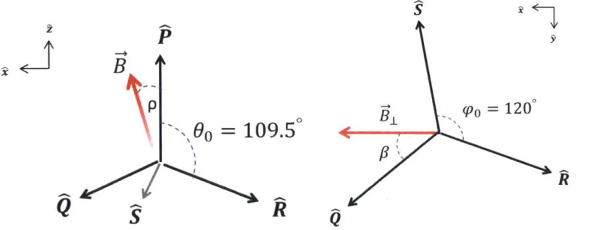
field onto the defect axis respectively. In calculating B11 and B1, however, the full 3-dimensionality of the diamond lattice must be maintained. Symmetry considerations dictate the diamond lattice to be tetrahedral. Defining the coordinate axes such that 2 lies along one of the bond axes (hereby denoted as P for Principle Axis4) and 1 lies along the transverse field direction, it is straightforward to calculate the parallel and perpendicular projections of B on the other 3 bond axes (hereby denoted as Q,

R, S5 ); the results are shown in Table 2. In calculating the results of Table 2, the

4

Note: All such references to "parallel" and "transverse" projections should be understood to be taken with respect to the Principle Axis

'Alternatively, one can consider the representations P -÷ (111), Q -+ (111), i - (i1i), S -(Mi1)

S

B,

P (po =120'

,1\0

= 109.5

Q

~

Rk

1S

Q

Figure 3-1: (Left) The tetraheldral geometry to be considered. The tetralhedral angle

is 109.5' and p is the angle between B and i. (Right) The tetrahedral geometry

projected into the trainsverse plane. The angle of' synnetry is 120' and 3 is the Offset of the tetrahedron with the x-axis, which is defied almg the transverse field

compllolent.

PB B,

B, Sill 0( cos0 + B c(Os 00 B2 -(B, sin 00 (0s

+

B co) s0))2

I? B, siln 0 cs ((3 + 'pO) + B, 0os 0 VB2 -(B1, sill 0 cos(83 + + )+ B, cos 0o)2

S B, sill 0( os( -3 'o) + B, (0s 0 \B2 - (B, Sill 0() cos(3 -'po) + B, (os 0))2

Table 3.2: The parallel and perpendicular projections of aii external magnetic field

B = B -+ B) onto the 4 possible defect axes. The angles 0(. 13 and ;o are defined

in the text.

following angles are defiined: 0o ~ 109.5' is the bond angle, '3 is the angle between

the transverse axis projection

Q

and the transverse field direction, ,o = 120' is the angular spacing of the three axes projections in the x-y plane. Fig. 3 - 1 provides a

visual representation of this coordinate configuration.

As can be clearly seen in Table 2. at most 3 tetrahedral axes can be considered svnmietricallv. in which the parallel and perpendicullar projections of the external

field will be equal. In this coor(illate sYsteim this occurs when B, = 0. These coordinates were chosen to make this feature manifest but no generality was lost in this coor(dinate defillition - there (loes not exist an external field orientation in which the parallel or perpendicular l)roj.ectionls onto every tetrahedral axis are identical.

The most symmetric configuration will always be when the external field is perfectly aligned with a tetrahedral axis.

With the projections defined, the total signal observed is a simple average over the 4 possible orientations with the assumption that the interactions between neighboring

NV centers can be neglected. Thus: I = R(Bf, Bf) (3.15) n where h F,

Q,

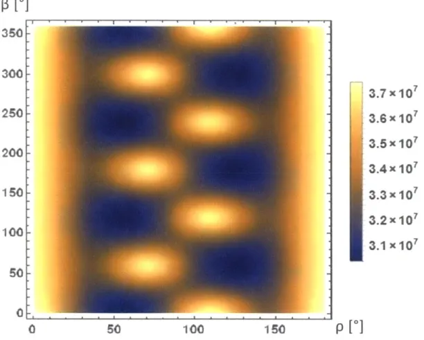
R, S.

Due to the trifold rotational symmetry of this geometry, a periodic signal profile develops in the presence of a finite transverse field, as can be seen in Fig. 3 - 2. Interestingly, in the quasi-parallel regime, in which B.

<

B,, the signal peaks occur

when the tetrahedral axes are anti-aligned with the transverse field. This is due to the bond angle being obtuse, so in the quasi-parallel regime a transverse field anti-aligned with a transverse tetrahedral axis has a larger parallel projection onto that axis than when aligned with it. As the system is rotated into the quasi-transverse regime, in which B.

>

B,, the aligned configurations transition from local minima

to local maxima as the minima shift towards the midpoint between the aligned and anti-aligned configurations. Finally, for completely transverse fields the aligned and anti-aligned configurations are perfectly symmetric, as the vector configuration is such that each - rotation maps B into its vertical image. That is to say, the angles formed₂ by B(O) and B(/+3 P) with the tetrahedral axes define vertical, congruent pairs. Note that this is always true for B1, but the symmetry is broken by the presence of a finite

B,. As B, is taken to 0 the vertical symmetry becomes realized. A full 47r rotation

map is shown in Fig. 3 - 3. In this figure, the discrete rotational symmetry of the NV tetrahedron is clearly visible with the bright peaks within the middle of the plot.

Normalized Intensity B = .03T, p = 20* /

/

50 100 150 200 2 B=.03T, p=85 Normalized Intensity 50 100 150 200 250 B =.03 T, p = 90' P) 50 300 350 300 350 Normalized Intensity 0.45 044 0.43 0.42 5 0 \ 50 100 150 200 250 300 350

Figure 3-2: Rotation profiles of the observed signal within the x-v plane. between B and :. increases from top to bottom from 20' to 850

.03T and F is set to 10. The intensities are nornalized to the p

to 90'. For all, = 0 intensities. 0.4535 0.4530 0 4525 0.50 0.48 0.46 0.44 0.42 angle B = p, the A,

p[ 0] 350 300, 250k 200 150 100 50 0L 0 50 100 1I50 3.7 x 107 3.6 x 107 3.5 x 107 3.4 x 10' 3.3 x 107 3.2 x 10' ,.1 x 10 p [0]

Figure 3-3: A full 4-r rotation map of the NV tetrahedron. /) is the polar angle of the external magnetic field and 3 is the azimuthal angle. JB is .01T and F is set to 10.

Chapter 4

Detection of Magnetic Fields

The aim of this work is to develop a method of detecting small magnetic fields. In many current methods of NV magnetometry an external bias field is applied to provide a reference for the unknown perturbing fields and in order to measure the unknown, small fields at the most sensitive working point. With this in mind, for the analysis that follows, the total magnetic field will be comprised of two terms: the known bias field and the unknown perturbing field, ie. B = 0 + b. The goal is to

calculate b in terms of B0 (a known parameter) and B-dependent measurement of the PL intensities. To do this, the problem will be broken up into 2 parts: developing a method to determine bl, and developing a method to determine b1. With this information the entire vector b can be reconstructed.

4.0.10

Parallel Fields

It is predicted that near the Level Avoided Crossing (LAC) regions the PL intensity will be highly responsive to small, transverse field perturbations, as can be seen in Fig. 4-1. The LAC regions are found when B, = hDgs/apg, hDe,/,pg, or B, ~ .103T,

.051T respectively. Indeed, close to these two points, our perturbative approach starts to break down.

tioralied ItenityNormalized Intensity B. = 0.0T B = 0.0 T sy=O0.002T 0.8 - B₁ = 0.002 T 0.6-0.4 - 0.50-002 004 0.06 0.08 0'10 0.2 0.02 O.04 0.06 0 08 0.10 0.12

Figure 4-1: A demonstration of the increased sensitivity of the NV center to

perturb-ing transverse fields around the LAC regions ~ .05T and ~ .T. On the left is the

single NN' case. while on the right the full ensemble is considered. Circled are the 3 symmetry pOIts about which a perturbing parallel field could he readily identified with the Imethods disclussed in the text. F = 10 in both cases. The small deviations

that occur near the LAC points are due to divergences in the coefficients o u that

develop as a manifestation of the Perturbation Theory and are not physical.

under small variations in B, - the 2 LAC regions and the midpoint between themi. It can be imagined that a biasing external field is established such that the NV center is placed within one of these 3 symietric regions. Then. being regions of high sensitivity. the magnitude of the parallel projection of the perturbing field can be determined from the difference in the observed signal and the signal predicted at the synn netry point. Only the magnitude of the parallel perturbation can be ininediately determined from the observed signal due to the syimmet rv of the region: however, the

sign of the perturbation call be obtained 1y shifting t he biasing field off the synunetry

point by a small amount and observing the change in the signal.

Mathematically. this is to say that at the svnmmetry poit = ( but elsewhere () and tls has a sign. Therefore 1y measuring the sign of , along with the direct measurement of S the parallel perturbation can be determined uniquely. This method of determining the parallel projection of the perturbing field will be referred to as the syunietric approach.

A different . umore intuitive approach would be to use the regions of maxinum

'Note that B = 0 is not considered in this analysis although it is a location where - vaiishes

and. when including the negative projections. indeed forms a symnetry point. The reason for its

oilission is that the curvature is poor at that location and thus from a practical consideration it is

slope rather than minimum slope as the biasing points as these regions will exhibit the largest sensitivity to parallel variations. However, the curvature profile of the signal is a function of the transverse perturbing field and so the specific location of maximum slope is not known a priori. The location of the local minima is, as it will always occur at the LAC point. Therefore it is recommended to use one of these extrema points as the bias points as they will be symmetric with any value of B2.

For small perturbations, an expansion can be performed around the symmetry points:

S(Bz) _ S(pi) + a2S (BZ - i) 2 + 4S (BZ - +) + (4.1)

02_Bz

Pi 2 4Bz i, 24

where pi denotes a symmetry point: - .05T, - .075T, or - .1T. Here only even

derivatives are nonzero when evaluated at pi due to symmetry considerations. For sufficiently small perturbations Bz - pi the higher order terms can be neglected and the perturbation can be solved for directly:

_

a

2

s

( B - pi)2 S(Bz) = S(pi) + a2 2 a2Bz P ₂ OS _2_ s - 2S (B - p A) OBz BZPi _{2Bz P} Therefore: / -1 b Z O S

₍

2 _{B z} / -1 AS 02S ~~BZ O2Bz

)

(4.2) ABz (2B

where b--B - p. Generally 2 - is a function of B_L and the optical pumping

parameter F and can be extracted by curve-fitting a signal profile such as that shown in Fig. 4 - 1. Unfortunately, B, is not a fully known quantity, as it will contain a perturbation as well. It is yet to be seen if there is an optimal F value which minimizes

the dependence of 2 on B,, in which case the dependence of the signal curvature

on B. can be neglectedptio good approximation and the symmetric approach can be applied in all experimental situations. An alternative approach would be to determine

B, before attempting to quantify b,; a method of measuring B, will be discussed later

in the section.

In Eq. 4.2, " is a measurable quantity; however by direct inspection of Fig. 4--1 it is clear that 9S is degenerate, but the locations of equal ' _{OB, B} are locations of unequal

S for Ib, < pil . Therefore it is recommended to observe the signal as well as the response of the signal to small changes in BO to determine the perturbation b,.

It is important to recall the presence of the other NV modes as a strong magnetic field parallel to one axis will be strongly transverse to the other axes. This effect can be seen in Fig. 4 - 1 for the ensemble case, where even in the absence of a finite B, there is a sharp drop in PL intensity. This is a manifestation of the effect seen in Fig. 2 - 3 in which an increasing transverse field drops the PL intensity. However, even in the ensemble case the LAC regions still demonstrate considerable sensitivity

to transverse perturbations. Furthermore, in this model the number of total NV centers used is a simple multiplicative factor in the signal calculation, so with enough

NV centers the signal can always be made sufficiently high to be detectable. As such,

even in the case of ensembles the symmetric approach will be applicable.

A potential problem arises, however, by biasing the NV ensemble around the symmetric regions, as the transverse fields experienced by the other NV modes are

of comparable strength to the zero-field splitting of the spin states. This model was

derived with perturbative methods assuming transverse fields will be small, and so selecting such strong transverse fields may interfere with the perturbative

approxi-mation. Therefore only the excited state LAC region will be used in the remainder of this thesis with the understanding that more accurate results can be obtained by more elegant approximation methods, such as expanding around the LAC regions, for example.

|

BO

Figure 4-2: The geometrv of the perturbing magnetic field. kfi is the angle between

the pertuibing field mnd the z-axis. and Q is the angle betweell the perturling field a11(d t he x-axis.

4.0.11

Transverse Fields

i3 Rotations

III considering transverse perturbatiois it is useful t properly define the geometry being considered. Fig. 4 - 2 demionst rates the iost general type of perturbilig field. In the figure. T is the angle betweein the perturbiing field and the z-axis, n1(d Q2 is the angle betweeln the perturlbig field an(1 the x-axis. To simplify the analysis. iii the presece of a )ertlllbing field the x-axis will be redefined to lie along the transverse proe(tion of the total magnetic field. This rotation can lbe alternatively viewed as a

chiage of .3 the anIglc betweein the tetrAhedral axcs 81d the x-axis.

Ali ambiguity exists when detcrilininhg the caiuse of all observed Z-shift 8s both the imiagni tude of the p)ertuIrblilng field 8A11d the orienlt at iol will (etermine the 3-sihift.

I11deed. fronm silmple geometry:

Sill _(4.3) BO + by cos ( or after rearrangeieiIt: B11 sin(Sj) (4 b) = (4.4) sin(Q - 6I)

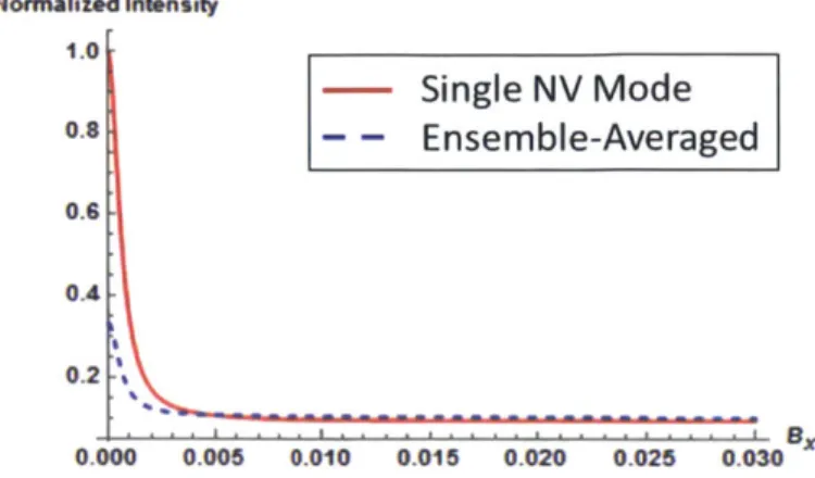
Nlormalized Intensity 1.0 Single NV Mode 0.8 - - Ensemble-Averaged 0.6 0.4 0.000 0.005 0.010 0.015 0.020 0.025 0.030

Figure 4-3: A plot (emonIstrating the effe('t of the tiransverse field on the observed

signal when the system is biased around the excited state LAC. Clearly the observed

signal approaels a stealdy vahie for B, > .002T. In generating this plot B. = .05T and I = 10.

versa. Note the case where BO = 0. In this situation Q (an lhe d(etermnine(l (mod 2)

by observing any transverse belavior. However in this case. sice Q will be equal to 6/3. 1)1 will b1e nllIdeterlineld.

Unfortunately, observinlg the periodic signal profile that charatterizes these i

ro-tations may prove to be difficult to realize experimentally if the system is to be l)iase(l in the quasi-transverse regime. As can he seen in Fig. 3 - 2 the magnitl(le of the oscillatory / profile is very small. and without (leveloplment of a f'ormal noise mo(el

it is unknown if these signal changes will be observalle. Clearly. to proeeed further

in the analysis it is requirel to (evelop a mnetllo(d of determining either 1)- or Q that piovi(des iore experimentally-feasible observatioms

Signal Curvature Profile

As can he seen in Fig. 4 -3. changes in the transverse field will cease to dire(tly infli-enee the olserved signal beginnling at relatively smiall magnitudes: the only influene the unknown transverse field will have on tle observed sigial will be in (etermlining

the ciirvature of the signal profile. Therefore a possible method of extractiig the transverse field mlagnitulde would he to measure the cirvature of the signal profile. amid then the parallel field magnitnde caii l)e (etermined as well as the transverse orient at iou Q.

Curvature --a Bz 4x1011 1 * 2x 10 -2x 10 -4x101 Curvature --4Kb1 1 . B = .002T B = .005T - B = .008T - 8z 0 0 @= 100 -

3=

450 S. 2 x 10"e* 0 0 0.01 .2 0.0 0 5 -21x101 -4x 10 1 1 BSS 2x 1011 8 B.) 0.01 0.02 0.0 005 -2 x1011 -4 x1011 0 7

F=

10

r= 50 F= 100 0 0.Q

Figure 4-4: A series of' plots depicting the dependencies of the signal curvature on

B.,. (Top). I (Middle) and F (Bottom). Clearly, a change in the transverse field

magnitude is the doiniaint cause for changes in the observed signal curvature. It is therefore proposed that bY mointoring the chaiges in the signal curvature the

82S Curvature -I x 10 2 8x 1011 6x1011 4x 1011 2x10 0 0.000 0.005 0.010 0.015 0.020

Figure 4-5: (Blue) A plot of the curvature of the sigial profile evaluated at B = .052T and F = 10 as a f'unction of B,. (Green) A fitted curve (to

.052

extract the leading order dependence of the signal curvatuire 10pon Br.

In general. the curvature of the signal profile will be a function of B,. B2. , and

F. Near the svnunetry points the (urvature of the signal profile is alIpproxilmlately constant with respect to B. (ie. =0. as i dictated by snnet The

the signal curvature will not be influenced by the presence of a Iparallel perturlbatioll. From Fig. 4 - 4 it is clear that the dominant source for changes in the observed signal curvature will he the presenc' of a traiisverse perturbation. Furthermore, the orientation of' that perturbation has little influence on the change of' curvature, only the mnagnitude of the perturbation will cause an observable change.

Fig. 4 - 5 plots the curvature of the excited state LAC as a function of B, To extract the B, dependence a curve was fit to this plot. shown in green in the figure.

F was set to 10 and .3 to 0. The functional form determined from this curve fitting procedure is:

)2 S 586038

OB2 (B, - .0005T )2

Since B = (BB 0 + b1 )2, b1 can be solved for as:

where B1, Os = 586038 ( + .0005T.

(9SObs)-/

Clearly when the observed perpendicular field matches the bias perpendicular field, the transverse perturbation is 0; however there is a negative solution (b1 =

-2B2 cos Q) predicted to exist as well. This solution is indicative of an underlying

symmetry that is physical and may very well become manifest if the bias transverse field is nonzero. This symmetry, which shall be referred to as the "3 symmetry" can be intuitively understood in Fig. 4 - 6, in which it is depicted as the "negative" solution for b1 given a positive angle Q or the "positive" solution for the negative angle (the latter will be the interpretation used in this analysis) 2. An alternate

method of understanding this symmetry is by considering the negative B, branch of the curvature plot in Fig. 4 - 5. As the curvature has no dependence on 3, in an unperturbed situation the transverse field can always be taken to be positive; however it could happen that a perturbation is perfectly anti-aligned with the bias transverse field and has a magnitude of 2B. In this case B1 is effectively mapped to

-B₁, which is an undetectable transformation with the sole observation of the signal

curvature. Thus these "0 symmetric" partners form a degenerate set, as there exists a continuum of allowed solutions due to the continuity of cos Q.

When it is not the case that the observed transverse signal is equal to the bias transverse field the solutions are split into 2 regions: BO < B1, Ohs and BO > B₁, Os.

These two regions can be made more obvious with the substitution B1, Os aBO

for an arbitrary a. Then, Eq. 4.6 becomes:

b =-BO cos Q B1 /a2 - sin2 Q (4.7)

In this equation it is obvious that b1 will be degenerate under the mapping a -+ -a. This is a manifestation of the rotational invariance of the system, and there is no loss of information by restricting a to be positive, as this is analogous to fixing the coordinate axes along the total transverse field. Furthermore, b1 will be double-valued with respect to the mapping Q -+ -Q as the RHS of Eq. 4.7 is an even function

2

Positive angle refers to an angle belonging to the angular region [- E, E] in which cos Q > 0

A-of Q.

jal > 1 Solutions

The region B'

<

B1, Obs corresponds to a > 1. In this case the term under the

radical will always be positive. To obtain the correct limiting behavior as a -÷ 1 the i in Eq. 4.7 must be handled properly. In doing this, the angular direction of b1 is limited to the quartercircle [0, 1] and b1 is confined to be strictly positive:

bi = -B (cos Q - a2 - sin2 Q) VQ : 0 < Q < (4.8)

Note that no information is lost by limiting the angular distribution of b1 to this subregion as the full degeneracy of the solution is recovered by calculating the double-valued solutions with the mapping Q -+ -Q for this region, and calculating the 3 symmetric partners. Given a transverse perturbation bi at a given angle

Rj

that solves Eq. 4.8, and a transverse bias field, the

/

symmetric partner can be calculated with the relationship:

bj bI + 2B- cosn (4.9)

The

/

symmetric set is then build up from the set of (ba, Qj) that constitute the positive solutions to Eq. 4.8.

It can be clearly seen that the

/

symmetric partners vanish if the transverse bias field is set to 0. This provides a simple means of removing the ambiguity in the observed curvature of the signal profile. Alternatively, the degeneracy can be partially lifted by probing the slope of the curvature profile in a similar manner as discussed for determining the magnitude of a parallel perturbation. If the slope is positive, then b1 - BO < 0; if the slope is negative, then b1 - Bj > 0.

jal < 1 Solutions

The region BO > B1, Obs corresponds to a < 1. Now, the term under the radical