Algorithms for design and interrogation of functionally graded material solids

Algorithms for Design and Interrogation of Functionally Graded Material

Solids

by

Hongye Liu

B.E., University of Science and Technology of China, 1993 Submitted to the Department of Ocean Engineering

and

Department of Mechanical Engineering

in partial fulfillment of the requirements for the degrees of Master of Science in Naval Architecture and Marine Engineering

and

Master of Science in Mechanical Engineering at the

MASSACHUSETTS INSTITUTE OF TECHNOLOGY June 2000

@ Massachusetts Institute of Technology 2000. All rights reserved

E

NG

NOV 2 9

2000

LIBRARIES

...

...

DeDartme t of Ocean Engineering ary 25, 2000 Certified by... ...

Nicholas M. Patrikalakis W.-1l %T!~d-i 1 Professor of Engineering

Certified by .... ... .. ...

Emanuel M. Sachs ichanical Engineering

A ccep ted by ...

Nicholas M. Patrikalakis, Kawasaki Professor of Engineering Chairman "mmittee -+1 on Graduate Studies A ccep ted by ...

Ain A. Sonin, Professor of Mechanical Engineering Chairman, Departmental Committee on Graduate Studies

Algorithms for Design and Interrogation of Functionally Graded Material

Solids

by

Hongye Liu

Submitted to the Department of Ocean Engineering and

Department of Mechanical Engineering on February 25, 2000, in partial fulfillment of the

requirements for the degrees of

Master of Science in Naval Architecture and Marine Engineering and

Master of Science in Mechanical Engineering

Abstract

A Functionally Gradient Material (FGM) part is a 3D solid object that has varied local material composition that is defined by a specifically designed function. Recently, research has been performed at MIT in order to exploit the potential of creating FGM parts using a modern fabrication process, 3D Printing, that has the capability of controlling composition to the length scale of 100 pm. As part of the project of design automation of FGM parts, this thesis focuses on the issue of the development of efficient algorithms for design and composition interrogation. Starting with a finite element based 3D model, the design tool based on the distance function from the surface of the part and the design tool allowing the user to design within a .STL file require enhanced efficiency and so does the interrogation of the part. The approach for improving efficiency includes preprocessing the model with bucket sorting, digital distance transform of the buckets and an efficient point classification algorithm. Based on this approach, an efficient algorithm for distance function computation is developed for the design of FGM through distance to the surface of the part or distance to a .STL surface boundary. Also an efficient algorithm for composition evaluation at a point, along a ray or on a plane is developed. The theoretical time complexities of the developed algorithms are analyzed and experimental numerical results are provided.

Thesis Co-Supervisor: Nicholas M. Patrikalakis, Ph.D. Title: Kawasaki Professor of Engineering

Department of Ocean Engineering

Thesis Co-Supervisor: Emanuel M. Sachs, Ph.D. Title: Professor of Mechanical Engineering Department of Mechanical Engineering

3

Dedication

4

Acknowledgments

Foremost, my sincere gratitude goes to my advisor Professor N. M. Patrikalakis for his expert guidance and strong support throughout the entire process. I also would like to thank Professor E. M. Sachs for his insight and valuable advice. I am also grateful to Dr. W. Cho, who helped me during my advisor's absence and provided useful comments on my thesis. My special thanks to Mr. T. R. Jackson, who put the first footprint on the FGM field that I followed. He showed me both warmth and wit throughout the project and gave me help in many various ways, such as providing me with sample models for testing. I also want to thank Dr. T. Maekawa, who helped me start research at MIT and showed me encouragement through out the last two years. I also cherish the experience of working with all the members of the Design Laboratory: Mr. G. Shen and Mr. G. Yu who helped me a lot during my tenure here apart from talking Chinese to me; Mr. F. Baker, Design Laboratory manager, without whose technical support my research would not be possible; Ms. K. Gunst for improving the English composition in an earlier draft of this thesis and all the rest of the Design Laboratory fellows whose friendship made my life at MIT easier. Financial support of this project was provided in part by the National Science Foun-dation (grant #DMI-9617750) and by the Office of Naval Research (grant

#N00014-96-1-0857). CAD models for this thesis were generated with SolidWorksT M, meshed with AlgorT M

Contents

2.1 Representation of FGM objects . . . . 2.1.1 Decomposition based method . . . . 2.1.2 Boundary representation based method 2.1.3 Extended cell-tuple structure based method 2.2 Design of FGM . . . . 5 2 3 4 5 8 9 12 13 . . . . 13 . . . . 14 . . . . 16 . . . . 17 19 19 19 20 20 21

CONTENTS

3 Finite element based FGM model

3.1 Introduction . . ... .. ... .. . .. . . . . 3.2 Data structure .... ...

3.3 Algorithm for the extraction of surface boundary 4 Preprocessing of finite element FGM model

4.1 Introduction . . . . 4.2 Computation of the boundary facets of the model . . 4.3 Construction of 3D bucketing system . . . . 4.4 Placement of the triangular facets into buckets . . . 4.5 3D digital distance transform . . . . 4.6 Identification of solid buckets . . . . 4.7 Bucketing vertices . . . . 4.8 Point location algorithm . . . . 4.8.1 Point membership classification (PMC) . . . 4.8.2 Identification of the object tetrahedron . . . 5 Design through distance functions

5.1 Introduction . . . . 5.2 Algorithm for efficient distance function evaluation . 5.2.1 Distance computation for a single query point 5.2.2 Distance computation for a single query point 5.2.3 Computation of the list of query points . . . 5.3 Design of FGM solids within given .STL boundaries 5.4

5.5

inside bounding box outside bounding bo3

Complexity analysis of distance function computation . . . . Experimental results comparison with exhaustive searching method . . . 6 Efficient evaluation of composition

6.1 Composition evaluation at a point using barycentric coordinates . . . . 6.2 Composition evaluation along a given ray at a given

resolution . . . . 23 23 25 26 29 29 29 31 33 35 37 38 39 39 40 47 47 48 48 49 51 51 52 55 63 63 64 6

CONTENTS

6.3 6.4 6.5

Composition evaluation on a cutting plane . . . . Volume integral of material . . . . Tim e analysis . . . . 6.5.1 Theoretical background . . . . 6.5.2 Time cost for the extraction of boundary 6.5.3 Time cost of point location algorithm . . 6.5.4 Time cost of ray casting algorithm . . . . 7 Implementation and numerical results

7.1 Implementation ... ... 7.2 Numerical results ... ...

7.2.1 Design from boundary ... 7.2.2 Design from .STL file boundary ...

7.2.3 Design within .STL boundary . . . . 8 Conclusions and recommendations

8.1 C onclusions . . . . 8.2 Recommendations . . . . A Development on FGMViewer

A.1 Extension to FGMViewer system . . . . A .1.1 Introduction . . . . A.1.2 M enu extension . . . . A.1.3 Major extension in classes . . . . A.2 Example of the use of FGMViewer . . . . B Geometric Algorithms

B.1 Algorithm for testing if a point is contained in a tetrahedron . . . . B.2 Algorithm for testing if a point is contained in a triangle . . . . B.3 Algorithm for testing if a line segment intersects a triangular facet . . . . . References . . . . 65 . . . . 66 . . . . 68 . . . . 68 . . . . 69 . . . . 70 . . . . 71 73 73 73 74 74 80 85 85 86 88 88 88 88 90 95 105 105 107 108 109 7

List of Tables

5.1 Efficiency enhancement on the example models . . . . 56 7.1

7.2

Parameters of the FEM example models . . . . 74 Performance of program on the examples . . . . 74

List of Figures

1-1 Functioning of LCC of 3D Printing, adapted from [16] . . . . 14

1-2 Information flow of FGM modeling system, adapted from [16 . . . . 15

3-1 Inheritance tree of FGMviewer object classes . . . . 25

3-2 Data Structure: Cube example . . . . 25

3-3 Data structure . . . . 28

3-4 Check to see if a face of a tetrahedron is interior . . . . 28

4-1 Preprocessing . . . . 30

4-2 Calculating the normal vector of a boundary facet . . . . 32

4-3 Bounding box with buckets . . . . 33

4-4 Distribute triangular facets into buckets . . . . 34

4-5 Example of chamfer distance transform: 0 is the feature pixel . . . . 35

4-6 Example of chessboard distance transform: 0 is the feature pixel . . . . 35

4-7 Digital distance transform . . . . 36

4-8 Chessboard DT Mask in 3D . . . . 37

4-9 Identify the signs of non-boundary buckets . . . . 38

4-10 Bucketing vertices based on the original bucket system . . . . 38

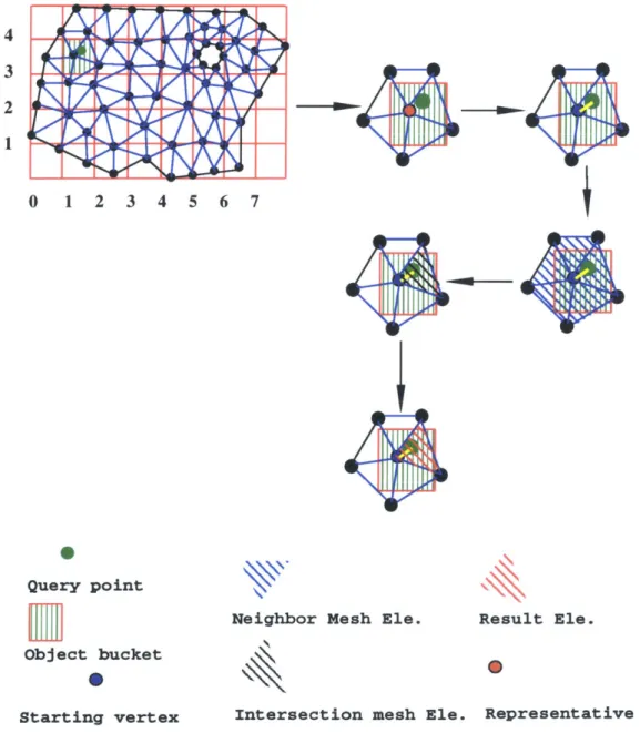
4-11 Check if a given point is inside the body . . . . 40

4-12 Intersection points coincide: da < db, choose facet a . . . . 40

4-13 Intersection points coincide: da = db , Kla - R > |7b -

RI,

4-14 Idea of locating the tetrahedron containing a given point . . . . 41

LIST OF FIGURES

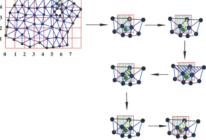
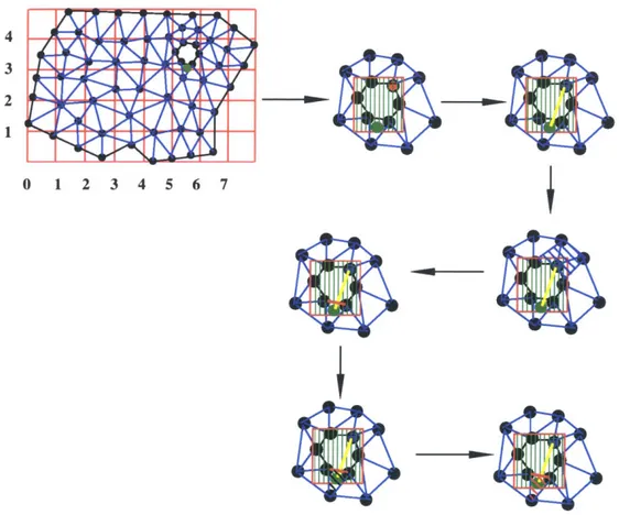
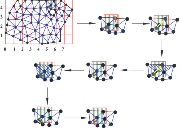
4-15 Case One: query point is connected with the starting vertex by a solid straight line segm ent . . . . 4-16 Case Two: Straight line segment between the query point and the starting vertex is not solid . . . . 4-17 Special Case: Starting vertex has to be changed . . . . 5-1 Idea of design FGM from the boundary of object . . . . 5-2 Compute exact Euclidean minimum distance for point inside bounding box 5-3 Euclidean minimum distance between a point and a triangular facet . . . . 5-4 Example A of distance function for points outside the bounding box of the

model ... ... ...

5-5 Example B of distance function for points outside the bounding box of the model ... ...

5-6 Identify the vertices that are contained in the given .STL boundary . . . . . 5-7 k is the chessboard distance of the query bucket to the boundary buckets;

number of non-empty buckets that the boundary occupied is 6n2

/3, where

n is the number of total buckets; buckets in the shaded area are nearest

non-empty buckets needed to be searched for the query point . . . . 5-8 Model 'Pill' . . . ..

5-9 Experimental results on 'Pill' . . . .. 5-10 Model 'Propeller' . . . .. 5-11 Experimental results on 'Propeller' . . . 5-12 Model 'Bracket' . . . .. 5-13 Experimental results on 'Bracket' . .

5-14 Model 'Sump' . . . .. 5-15 Experimental results on 'Sump' . . . . 6-1 Evaluate composition at a given point 6-2 Evaluate composition along a given ray 6-3 Parametric cutting plane . . . . 6-4 Tetrahedron natural coordinates . . . .

10 44 45 46 47 49 50 51 57 58 58 . . . . 5 9 . . . . 5 9 . . . . 6 0 . . . . 6 0 . . . . 6 1 . . . . 6 1 . . . . 6 2 . . . . 6 2 . . . . 6 4 . . . . 6 5 . . . . 6 6 . . . . 6 6

LIST OF FIGURES 7-1 7-2 7-3 7-4 7-5 7-6 7-7 7-8 7-9 7-10 7-11 7-12

7-13 Design within STL boundary according to the distance to the 7-14 Slice of above at Z=20 . . . .

Pill ...

Bracket with a hole ...

W idget . . . . Pill composition data ...

Pill slice at z = 0 ...

Bracket's composition data . . . . Bracket slice at z= I. . . . . Bracket slice at z = 3. . . . . Widget composition . . . . W idget slice . . . . Design from a stl file, range (0, 90) Slice at Z = 20 . . . .

7-15 Design first through distance to STL mesh (0-90) then design within that STL boundary through distance to that STL mesh (0-40) . . . . 7-16 Design first through distance to STL mesh (0-90) then design within that STL boundary through distance to that STL mesh (0-40) . . . . 7-17 Slice (Z=20): Design first through distance to boundary (0-90) then design within a STL boundary through distance to that STL mesh (0-40) . . . . . 7-18 Slice (Z=10): Design first through distance to boundary(0-90) then design within a STL boundary a constant material . . . . A-1 Inheritance tree of FGMviewer object classes . . . . A-2 Inheritance tree of mfunction classes . . . . B-1 Test if a given point is contained in a tetrahedron . . . . B-2 Test if a given point is contained in a triangular facet . . . . B-3 Test if a line segment intersects a triangular facet . . . .

. . . . 75 . . . . 75 . . . . 76 . . . . 76 . . . . 77 . . . . 77 . . . . 78 . . . . 78 . . . . 79 . . . . 79 . . . . 80 . . . . 81 STL mesh. . 81 . . . . 82 82 83 83 84 91 94 105 107 108 11

12

List of Symbols

Symbol Definition

n Number of buckets in the bucketing domain of the object

nbf Number of boundary facets of the object

nt Number of tetrahedra in the tetrahedral mesh of the object nv Number of vertices in the tetrahedral mesh

nx, ny, nz Number of buckets along axes x, y, z respectively

l, lY, lz Length of object domain along axes x, y, z respectively

lb Side length of one bucket

X*, y z* Coordinates of a point in the bucketing frame

Bijk Bucket that is indexed i,

j,

6i, 6j, 6k Absolute differences between two buckets in terms of the indices of the buckets

Bq The bucket that contains the query point

ListBnr _{The list of nearest non-empty buckets relative to} Bq

T The total time cost for an algorithm

Tyre The time cost for preprocessing step in an algorithm

Ti The time cost for distance computation for the ith query point

Ef Efficient enhancement factor of distance function algorithm compared to exhaustive searching method

PT Experimental result of preprocessing time

u, v, w, rj Barycentric coordinates of a query point in a tetrahedron

6t Resolution in parametric form

Pa Integral volume ratio of material a in the object

Vm Volume of tetrahedron indexed m in the tetrahedral mesh

bk1 Structure constant of a homogeneous incidence structure from

Chapter 1

Introduction

1.1

Background

Solid Freeform Fabrication (SFF) technology, also called Rapid Prototyping is a modern Computer Aided Manufacturing technology through which prototypes, parts, and tools are built in an additive fashion directly from CAD models. Among various SFF processes, the 3D Printing at MIT, the Selective Laser Sintering at University of Texas and the Shape Deposition Manufacturing at Carnegie Mellon and Stanford Universities are among the most prominent. 3D Printing [28] is one of the SFF manufacturing processes in which a 3D structure is built layer by layer and completed near-pointwise. Compared with the other SFF manufacturing processes, 3D Printing not only possesses the advantage of producing new complex solids that traditional technologies such as subtractive machining, forming or casting can not make or make efficiently, but also has better flexibility in exercising control over composition. Via selective placement of different materials available to the machine, 3DP can achieve near-pointwise local composition control (LCC). A 3DP machine exercises LCC in a fashion similar to ink-jet color printer printing which is illustrated in Figure 1-1.

The LCC characteristics of 3DP manufacturing opens the door to the production of material with graded local composition that is called Functionally Graded Material (FGM). FGM has many possible applications such as structural property control, thermal property control, medicine delivery control, multicolor visualization, etc.

In current rapid prototyping practices, designers usually create a model using a

CHAPTER 1. INTRODUCTION

finish st

--v

Spread powder Apply binders Lower print bed Finished part Figure 1-1: Functioning of LCC of 3D Printing, adapted from [16]

tional CAD system and obtain a tessellation of the boundary of the model in the form of a collection of triangles. The file format storing the model is an industry standard known as .STL [22]. The trimmed surface model is then processed into machine instructions to control the fabrication.

In order to fabricate an FGM part through LCC, it is necessary to build a CAD solid modeling system by capturing graded material composition and generating appropriate ma-chine instructions. The traditional CAD systems do not facilitate such an implementation because the solid model they deal with is a digital representation of only the external geom-etry of a physical object and therefore do not permit easy LCC manufacturing. In order to go further to represent, design, and process models with graded material compositions, var-ious research groups have investigated the extension methods concerning representing FGM from traditional solid representation. Among them T. R. Jackson et al. has proposed and

developed a prototype FGM representation using an extension of cell-tuple data structure [5] with volumetric, FGM cells [16].

Regardless of what representation method is chosen, in order to represent graded ma-terial variation and plan the machine processing, the model is necessarily divided into sub-regions. At M.I.T. , a method for piping information from CAD system to the 3DP machine has been developed in order to produce an FGM part, see Figure 1-2.

1.2

Motivation and objectives

Although with the developed cell-tuple FGM modeling method, the users are able to capture their ideas as models with graded compositions and then convert these models into machine instructions for their fabrication, the modeling system also needs to be efficient in terms 14

CHAPTER 1. INTRODUCTION

Geometry intent Composition intent

3D gemetry3D geometry 3D geometry and composition Machine instructions Design rules

Figure 1-2: Information flow of FGM modeling system, adapted from [16]

of memory and speed of execution. For example, beginning with a model derived from triangulated, STL model, the expected FGM model with uniform mesh of tetrahedra is expected to be large. "In case of a cube subdivided into a structured mesh of tetrahedra, the relationship between the number of tetrahedra nitet in the mesh and the number of boundary facets nb in the STL model is: nitet = 5(nb/12)3/2. For a small STL model of only 9408 facets, the corresponding FGM model of cube with uniform mesh would have 497225 cells of dimensions 0 to 3 (24389 vertices, 138852 edges, 224224 faces, 109760 tetrahedron regions) and requires a graph with 2690688 nodes to maintain the topology [16]." Estimating from this observation, the model from a large STL model will have prohibitive large size. Therefore, as stated before, for a large model it would be very useful to define a finite element mesh FGM cell for graded composition in order to reduce the memory cost for complete topology storage. Because it is desirable to achieve overall efficiency in terms of both memory and speed, we do not want to discard all the topology information that can help with faster query algorithms.

In addition, although the prototype system that Jackson et al.[15] developed based on

cell-tuple struture provides a useful tool for designing compositions in terms of distance from a fixed feature in a straightforward manner, the efficiency of the distance function becomes an issue especially when designing from the boundary of a model. For example, the algorithm for assigning the control compositions must compute the minimum distance from each query point (corresponding to a control composition) to the boundary of the model. With the potential of a model having a large number of query points, the exhaustive

CHAPTER 1. INTRODUCTION

searching through all the boundary facets may be prohibitively time consuming.

The CAD modeling system not only needs to provide design tools, but also needs to provide functionality for the user to evaluate the properties of the FGM model. The eval-uation of composition of FGM will be most important for either the visualization or the post-processing of the FGM model. Query of the composition may be in the form of the query for a point, a ray, or a plane. Since the composition of the model is represented by finite number of control compositions, given for an arbitrary point inside the solid, it is necessary to evaluate the composition at that point using interpolation of the control compositions.

As part of the CAD system project of FGM for 3DP, this thesis work addresses the above efficiency problems and gives an effective solution.

1.3

Summary of methodologies

In order to model a general FGM cell with a finite element mesh efficiently, it is necessary to keep some of the topology information of the mesh. In the case that the model is converted from a tetrahedral mesh, the incidence relationship from a node to its incident tetrahedra is maintained, which helps to speed up the querying algorithms.

In this thesis work, an efficient distance function algorithm is developed based on the "Bucketing" algorithm and the digital distance transform of the buckets.

In our approach of the composition evaluation of an FGM model, an efficient point location algorithm is developed to identify the sub-region (tetrahedron) corresponding to the query point, and the control compositions of that tetrahedron are used to interpolate for the query point. An efficient point location algorithm is developed based also on the "Bucketing" method and the finite mesh structure with certain topology information and boundary facets. Once an efficient point location algorithm is available, the composition evaluation at a point is done via linear interpolation using barycentric Bernstein basis polynomials. Composition evaluation along a given ray or on a given plane can be easily developed by extending the composition evaluation algorithm at a point.

CHAPTER 1. INTRODUCTION

1.4

Thesis organization

Chapter 2 begins with a brief review of recent work on the representation and design of FGM objects.

As a memory saving choice for FGM object representation, a finite element based FGM model is described in chapter 3. In an attempt to facilitate efficient query algorithms, the finite element structure maintains certain topology information. In addition, the data structure and its relationship with a development environment of FGM modeling, design and processing is described. At the end of chapter 3, an algorithm for the extraction of the boundary facets is presented.

Chapter 4 contains the preprocessing methods of the finite element based FGM model that are essential in helping generate efficient queries used for both the efficient distance evaluation and efficient point location algorithms. The preprocessing of the model includes bucket sorting of the boundary facets and vertices, 3D digital distance transform, solid bucket identification and the point location algorithm. The point location algorithm is included here not only because it is closely related with the preprocessing method but because the algorithm itself is developed in order to enhance the efficiency of composition evaluation of the FGM model; therefore, the point location algorithm is also considered a preprocessing procedure.

In Chapter 5, the algorithm for design of FGM through the efficient distance function is presented. As the spirit of this algorithm, the efficient evaluation of the distance function to the surface of the model is analyzed and the experimental comparison with exhaustive searching method is given.

Chapter 6 provides the method for the evaluation of the composition of the FGM model, which is also useful in the rendering of the model. In addition, time complexity analysis of the method is presented.

The implementation of all the algorithms from Chapter 3 to Chapter 6 is given in Chapter 7 with numerical results on several sample models.

Chapter 8 concludes the thesis and provides potential directions for related future work. Appendix A describes the implementation and integration of our algorithms into a 17

CHAPTER 1. INTRODUCTION 18

software called FGMViewer along with a user's manual.

Chapter 2

Review

2.1

Representation of FGM objects

In order to achieve FGM object fabrication, researchers in SFF community have been inves-tigating the method of representing FGM objects by extending existing CAD representation methods. The followings are some of the proposed methods. Among them, a cell-tuple struc-ture based method has been developed sufficiently along with methods to transmit data to

the 3DPTM machine.

2.1.1 Decomposition based method

The traditional decomposition models represent objects by subdividing space into multiple sub-regions. This method is often used in finite element analysis, medical data rendering and so on by attaching physical properties to individual sub-regions. In order to repre-sent FGM objects, the model can be enriched by attaching material information to each sub-region [25]. This method has the advantage in that there are a lot of volume graphics algorithms available, though the design and interrogation of FGM objects using this rep-resentation is cumbersome because it does not maintain topological information about the model. In addition, this method does not have the generality of describing free-form curves and surfaces; similarly, it is not easy to represent arbitrarily graded composition using this method. In terms of data exchange, methods compatible with the neutral standards such as IGES [12], STEP [13] need to be developed to exchange models based on the decomposition

CHAPTER 2. REVIEW

method. In the case of representing FGM with a large constant material composition area, using uniform decomposition (e.g. in a tetrahedral mesh) is not memory efficient compared to boundary representation and an abstract structure such as the cell-tuple representation.

2.1.2 Boundary representation based method

In current CAD systems, the boundary representation (B-rep) is most used because of its flexibility in modeling complex geometry precisely. Boundary representation describes solids in terms of their bounding entities such as shells, faces, loops, edges and vertices [2]. As described in Chapter 1, the traditional B-rep models do not contain material information explicitly. Based on one of the traditional B-rep models, the r-sets model, a heterogeneous solid model (rm-set) is developed as a finite number of subdivisions with each subdivision being a material domain with a defined material variation function [19]. This approach is first proposed for representing composite models (material within each domain is con-stant) with the model constructed by using Boolean operators. Although in principle this method is able to represent graded composition by choosing varied material function for each domain, the transformation of the analytic composition variation information to spe-cific process plans has not been presented.

2.1.3 Extended cell-tuple structure based method

In the traditional cell-tuple structure, a model M is represented in terms of a set of cells C where each cell ck is a topological entity such as a vertex, edge, face or region. Here the edge and face can be arbitrary curved-entities and the region can be any valid manifold

hemeomorphic to a topological open ball. All the component cells are connected through a graph T. Geometrically the model is determined by the geometric information associated with each cell (expect the region). A cell-tuple data structure can be constructed using data from a neutral standard format with or without approximation. Without approximation, the cell-tuple structure will be able to precisely describe the geometry of the original solid. "To represent an FGM model within the cell-tuple structure, composition information as well as geometric information is also associated with each cell. The information begins with the concept of a material space M spanning the dm primary materials available to 20

CHAPTER 2. REVIEW

an SFF machine capable of LCC. The composition of the model is represented as a vector valued function M(X) defined over the model's interior. Each component mj of m repre-sents the volume fraction of the corresponding material in the material system present at point XF within the model" [16]. As a general abstract data structure, cell-tuple structure based FGM model has the possibility of describing graded material composition of arbitrary degrees. And because of the generality of its cells, one can even construct a cell of finite-element mesh, which is important for a large complicated model. In order to provide the capability of describing how the FGM composition varies within a solid, the FGM modeling has to decompose the interior of the solid into simpler sub-regions and each sub-region has the information about the composition variation in its domain. Theoretically, models can be arbitrarily subdivided into topologically simpler domains over which shape and compo-sition functions can be more readily defined analytically. To simplify the procedure, the prototype FGM system at MIT begins with models subdivided into tetrahedral meshes, and the conversion from traditional solid models to FGM system is done by employing standard meshing algorithms.

2.2

Design of FGM

The design of FGM is another important phase in the whole FGM modeling process. In one of the definitions of "Solid Modeler", a solid modeling system is defined as a computer program that provides facilities for storing and manipulating data structures that represent the geometry of individual objects or assemblies [21].

Currently, there are two different categories of FGM design approaches. One is design in top-down fashion, in which the CAD model is decomposed into simpler geometry sub-domains, and then the designer designs graded composition over all the sub-domains. For example, the system developed at MIT provides composition functions, especially a graded composition in terms of volume fractions of the material over the domain of each sub-region. Over each cell's domain Ck, the shape and composition is formulated in terms of a set of control points and control compositions which are blended with the barycentric Bernstein polynomials [11]. The degrees of control points and control compositions are determined 21

CHAPTER 2. REVIEW

according to the degree of variation of the geometry and composition of cells. With each control composition of the model representing a degree of freedom, the design of the FGM parts becomes the procedure of assigning values to each and blending over the whole domain. The design tool that helps in design of control compositions in terms of distance functions to a selected feature is developed. The selected feature may be a fixed reference in the model space, such as a point, line or plane, or a feature of the model, such as a particular face or its entire boundary, or an independent boundary shell in .STL format. After a feature is selected, the designer specifies a variation for the FGM in terms of distance from the feature: m(Y*) = M(r(Y*)), where r is the distance of a query point x* from the reference feature. Next, the design tool automatically visits and assigns the control compositions for each cell, and in this way defines the composition over the whole model domain. The other approach is to design FGM by composition using a library of predefined components. The composing of different components can be done by using operators specific to the chosen data structures. This approach has not yet been fully explored but preliminary results are reported by researchers at Stanford University and the University of Michigan [3][26].

Chapter 3

Finite element based FGM model

3.1

Introduction

In Chapter 2, we have reviewed three proposed approaches of representation of FGM objects and one can see each method has its own advantages and disadvantages. In terms of generality, flexibility and approximation precision, the B-Rep and Cell-Tuple approaches are obviously better choices. But once we have the objective to provide the whole pipeline including modeling, design of graded material composition and process planning into SFF fabrication processes that are capable of LCC, it is necessary to discretize the model either before the design phase, during this phase, before the process planning or embedding in the process planning phase. The choice of designing composition before subdivision will limit the design function in the scope of analytic function; subdividing before the interactive design of composition cannot take into account the user's design intentions, etc, therefore it is not ideal either; the ideal method therefore is to subdivide the model in the process of design according to user's design intention and design rules that are defined in an expert system.

Although the discretization is a very important issue in FGM modeling, it has not been studied in depth yet. For example, in order to achieve FGM production, the approach based on B-rep (extended r-set) method [20] [26] hasn't addressed automatic subdivision issues and has only achieved composite composition, which means piecewise constant ma-terial composition in each sub-region. In the case of graded composition, the proposed

CHAPTER 3. FINITE ELEMENT BASED FGM MODEL

design method [18] is to attach an analytical function to each sub-region, which will leave further discretization to process planning, and also incur further problem of modeling de-signer's (users) intuitive design intention in terms of analytic function in each sub-region. In comparison, the approach based on cell-tuple structure [16] has simplified the subdivi-sion procedure via subdividing the traditional CAD model in neutral standard format into meshes of simpler subdivisions using commercial software, as described in Chapter 1 and 2. This approach has a memory bottleneck in the case of large dense uniform finite ele-ment mesh input, because a cell-tuple structure maintains complete topology information between the topology entities including internal structures.

From the above analysis, we can see the modeling of FGM still has a lot of open questions and problems to solve, therefore it is difficult to draw a conclusion with an optimum solution. When the development of a cell-tuple structure based on FGM modeling met the obstacle of memory bottleneck for large mesh input, questions were raised such as "Which is the best choice; cell-tuple alone, finite element alone, or a mix of these two?". In this context, research was carried out on using a finite element based approach to represent FGM.

It was decided to develop algorithms based on a finite element approach because both the finite element based approach and the cell-tuple with finite element based approach involve a finite element subdivision and it turns out that a finite element based structure is easier for implementation. Under the assumption that we want to achieve efficiency based on a decomposition approach, it was also decided to keep some of the topology information of the model for better efficiency in query algorithms. Meanwhile, as an effort of developing a newer approach of the FGM system, an exploratory environment of modeling, designing, and post-processing of FGM has been developed and a pure finite element representation implemented. Therefore it is natural to place this thesis work into that environment. Fig-ure 3-1 demonstrates the inheritance tree of the finite element mesh with some topology in this thesis from the implemented classes of that exploratory environment [14]. Following this introduction, the data structure used in this work will be described and also the algo-rithm of extraction of the boudary facets from the input finite element mesh is presented. Appendix A. 1 also gives the extension of the computer-user interface developed in this work. 24

CHAPTER 3. FINITE ELEMENT BASED FGM MODEL

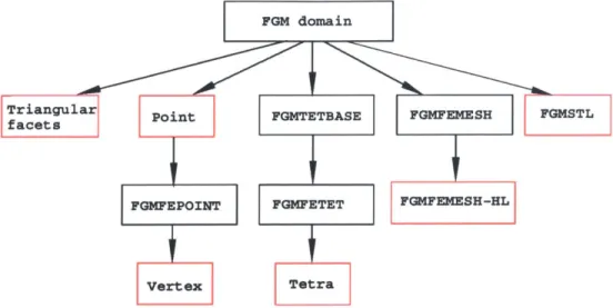
FGM domain

Trianular rPoint FGMTETBASE FGMFEMESH FGMSTL

FGMFEPOINT FGMFETET FGMFEMESH-HL

Vertex Tetra

Figure 3-1: Inheritance tree of FGMviewer object classes

7 6

Tetrahedra of the model: Vertices of the model: 2 - -. 1={ 2,7, 8, 9} 1 E (2, 4, 6, 7, 8) 2{ 1, 2, 7,, 9 ) 2 G ( 1, 2,3, 4, 5) 3=12, 4, 8, 9) 3E (5) 4=1 1, 2, 4, 9) 4(3, 5, 6,9) 5= 12, 3, 4, 8) 5 G (6, 8, 9, 10) - ...-- : 6=1 1, 4, 5, 9) 6G (7, 8, 10, 11) 7=1 1, 6, 7, 9} 76 ( 1, 2, 7, 11) 3 8 ={ 1, 5, 6, 9) 86 (1, 3, 5, 9, 10, 11) 9 =1 4, 5, 8, 9) 96 (1, 2, 3, 4, 6, 7, 8,9, 10, 11) 10 = 1 5, 6, 8, 9) 11=16, 7, 8, 9)

Figure 3-2: Data Structure: Cube example

3.2

Data structure

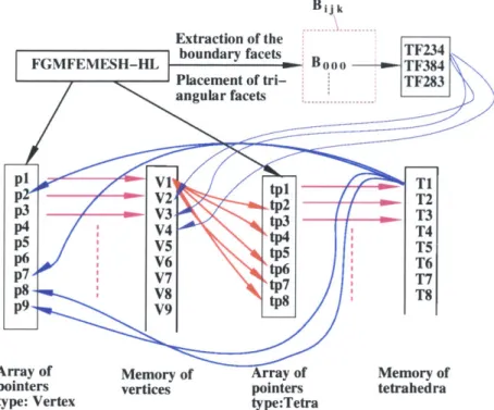
The data structure of an efficient finite element based FGM model is presented here. Specif-ically, the data structure maintains an array of object "Vertex" pointers, an array of objects

"Tetrahedron" pointers, a list of indices of the tetrahedra that are boundary tetrahedra and a bucketing system. The bucketing system has n number of buckets and several bucketing parameters, where n is the number of boundary facets. Each bucket is associated with a list of triangular boundary facets and a list of vertices. An object of "Vertex" is associated with the geometric position of the vertex, a queue of incident tetrahedra indices and the material composition vector at that vertex. A tetrahedron has an array of four vertices,

CHAPTER 3. FINITE ELEMENT BASED FGM MODEL

and the status of each tetrahedron with respect to it being a boundary tetrahedron or not; in addition, if a tetrahedron is a boundary tetrahedron, the status of each face is stored according to the face being a boundary face. Figures 3-2 and 3-3 demonstrate the data structure for representing a model of a cube split into 11 tetrahedra.

3.3

Algorithm for the extraction of surface boundary

Because the finite element mesh does not have explicit surface boundary storage, it is necessary to extract the boundary information for future use. This is done in the process of initialization of the data structure. The initialization of the data structure and the extraction of boundary procedures are as follow:

Algorithm 1 initDataStr(FEMesh M); initialize the data structure from finite element mesh generated from Algor

1: for each node Nd E M do

2: construct new node newNd E newM;

3: for each tetrahedron T E M do

4: initialize newT E newM; 5: set each face status as exterior;

6: set four associated vertex pointers to newT; 7: for each of the four vertices do

8: add newT to the corresponding incidence list; 9: for each face F C newT do

10: check if F is interior and set the status; >see Algorithm 2 11: initialize BTL; >BTL is the boundary tetrahedra list

12: for each newT C newM do

13: if newT is boundary tetrahedron then

14: add newT to BTL; 15: else

16: delete face information.

Based on the assumption that the finite element mesh is conforming, for an interior face, the two incident tetrahedra should appear in all the three parent tetrahedra lists according to the three vertices of the face. Therefore, the two incident tetrahedra should each appear 3 times in the combined list of the parent tetrahedra lists of the three vertices. Under the above assumption and observation, the algorithm for checking if a face of a tetrahedron is interior is done as follows:

CHAPTER 3. FINITE ELEMENT BASED FGM MODEL

Algorithm 2 isInterior(faceNo F, Tetrahedron T); check if F G T is interior face 1: if F has the status as interior then

2: return; 3: else

4: for each vertex E F do

5: check out the incidence tetrahedra list;

6: if the three incidence tetrahedra lists overlap then 7: put the three lists into one list;

8: count the occurrence of each element of the list; 9: if there exists T1 / T counted 3 times then

10: set F as an interior facet in T and T1;

11: else

12: status remain; 13: else

14: no, the face status remains unchanged.

Figure 3.3 shows how the algorithm of checking interior faces works.

CHAPTER 3. FINITE ELEMENT BASED FGM MODEL 28 Bijk Extraction of the boundary facets TF234 FGMFEMESH-HL .No-: 0 -1 - TF384 Placement of tri- :TF283 angular facets ... ... p9 V 1 T1 p V2 tpeT2 p3 V3 - D trt T3 p4 V4 ,tp3 T4 p5 V5 ( 35 T5 p6 V6 -tp5 T6 p7 V7 T p8 V8 t8T8 P9, V9 p

Array of Memory of Array of Memory of

pointers vertices pointers tetrahedra

type: Vertex type:Tetra Figure 3-3: Data structure

Vertices Parent TetraList Integer Interval 2 1 ( 1,2, 3,4, 5) [ 1, 51]

0

Face No.2 of the Tetra-hedron No.1.

8

J(

9, 10, 11)

Do if the three integer intervals overlap:

a: Count the occurence of elements

in the three TetraLists;

Tetrahedron No. I and No. 3 counted 3 times.

b: Face No. 2 of Tetrahedron No. 1 is incident to both Tetrahedron No. I and No. 3, i.e. set face No. 2 as interior facet.

Chapter 4

Preprocessing of finite element

FGM model

4.1

Introduction

In order to improve the efficiency for computing minimum distance from a query point to the boundary of the model or a given .STL boundary, a preprocessing method using bucket sorting technique [8] and digital distance transform [4] is employed. After such preprocessing, computation of the Euclidean distance for a specific query point has to be done with respect to triangular facets in the buckets which have the nearest digital distance to the query point. Figure 4-1 graphically illustrates this preprocessing. Based on the bucketing processing, an efficient 'Point Location' algorithm is developed, which is very essential to the efficient evaluation of the composition of an FGM model. Because the 'Point Location' algorithm is very much related with the 'Bucketing' processing, it is also placed in this chapter together with the 'Bucketing' preprocessing.

4.2

Computation of the boundary facets of the model

After the initialization of the data structure, the boundary tetrahedra list is obtained as described in the previous chapter and each boundary tetrahedron has its boundary facets identified explicitly. Based on this boundary tetrahedra list, an array of triangular facets is

PREPROCESSING OF FINITE ELEMENT FGM MODEL

boundary

Solid Model

0

0

0o

0

0

0

0 0

₀₁

_0/

Digital distance

transform

S0

0

0 0 0

-O 0

11

1

1

0

1

0

10

1

Identify sign of digital distance

Bounding domain

with buckets

Distribute the boundary entities

Figure 4-1: Preprocessing

CHAPTER 4. PREPROCESSING OF FINITE ELEMENT FGM MODEL 31

constructed with their normal vectors calculated.

Algorithm 3 getTriFacets(BndTetList BTL); construct the boundary facets list from boundary tetrahedra list

1: initialize TriFacetList;

2: for each boundary tetrahedron BT E BTL do

3: for each F (E [0, 3]) of T do

4: if F is a boundary facet then 5: initialize Tri;

6: calTrifrmF(Tri,F,T); 7: add Tri to TriFacetList;

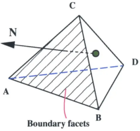
Algorithm 4 calTrifrmF(Triangle Tri, faceNo F, Tetrahedron T) refer to Figure 4-2 1: set vertices of Tri;

2: identify vertex D;

3: if CA x CB CD > 0 then 4:

|CAxCB

>N is the normal vector of Tri 5: else

6:

- CA x CB

CA x CB

4.3

Construction of 3D bucketing system

Given n numbers in [0,1) ,K1, K2, .. .K, the bucketing technique [8] in one dimension divides

the interval [0,1) into n equal-sized subintervals, or buckets, and then distributes the n input numbers into the buckets. The analogous bucketing process in 3D [6][7] is essentially dividing the bounding box of the model into equal sized cubic sub-regions (buckets). Given the number of facets of a solid model (n), we build the bucket system such that n, x ny x nz =

n, where ni, ny and nz are the number of buckets along the Cartesian coordinate axes x, y, z

CHAPTER 4. PREPROCESSING OF FINITE ELEMENT FGM MODEL 32 C

N

Figure 4-2: Calculating the normal vector of a boundary facet

build cubic buckets, nx, ny and n, should obey the following formula

Y . ; lx .lz lx -ly

that relates them to the dimension lengths of the object, and therefore the side length of one bucket is

b _Z I -Fn

Apparently lx , ly and lz can be found by computing the minimum of xi, minimum of yi,

minimum zi, maximum of xi, maximum of yi, maximum of zi. After we build the bucketing frame system that originates at (Xmin, Ymin, zmin), we need to transfer the old coordinate position of each vertex of the object to its new position in the new frame system. The transform formulae are as follows

XX - min YY - Ymin; Z*= z - Zmin

lb lb lb

In the bucketing system as in Figure 4-3, a bucket that is the ith from left, the jth from front and the kth from the bottom is denoted Bijk.

CHAPTER 4. PREPROCESSING OF FINITE ELEMENT FGM MODEL

Figure 4-3: Bounding box with buckets

4.4

Placement of the triangular facets into buckets

The purpose of this procedure is to build the reference for each triangular facet on the object boundary to the buckets that intersect it. For one single facet, the intersection detection is divided into three phases: the first step is to find buckets that intersect the vertices of the facet; the second step is to find buckets that intersect the edges of the facet, when there is edge intersecting more than two buckets; the third step is to find buckets that pass through the facet without intersecting the edges of the facet. All three steps are illustrated in Figure 4-4.

STEP 1 Find buckets that intersect the vertices of the facet

This can be done easily by taking the floor (or integer part) of the bucketing co-ordinates of each vertex. The resulting integer coco-ordinates are the bucket indices.

i = [x*J, j = [y*J,k = [z*J

STEP 2 Find buckets that intersect the edges of the facet

After the buckets that intersect the vertices of the facet are obtained, we can trace on each edge from one end point bucket to the new bucket that intersects the edge until the other end. This can be done by identifying the side of the six sides of the current bucket that is intersected by the edge in the tracing procedure. If the current bucket is intersected at right, the index i of the new bucket should be increased by

5WW1WWWWW_ - - -- -- .- _ -",

CHAPTER 4. PREPROCESSING OF FINITE ELEMENT FGM MODEL 34

1, while decreased by 1 if intersected at left. Similar operations can be done if the current bucket is intersected at other sides.

Bucket that

k

VP 2 Projecticn in j-k plame ich has the larges

projepticno area.

No.k sqarstctally irulrb rMi the

projected trim f

VP'

VP₃

VP

2

Figure 4-4: Distribute triangular facets into buckets

STEP 3 Find buckets that pass through the facet but not intersect the edges of the

trian-gular facet

The detection work is divided into two parts. First, we find two of the three indices of each such bucket by projecting the triangular facet along its maximum normal di-rection, which means the direction that the normal vector has the maximum value of projection area. For example, if the normal vector to a facet is (n,, ny, nz) and

1nx ;> |nyI, In,|, we project the triangular facet into y - z plane, and then first find

the index j, k of the bucket if square (j, k) is completely inside the projected triangle.

Since we have found buckets that intersect the edges, we can just scan for each pos-sible k to see if there are some jo that satisfies j1(k) < jo < J(k), where jj(k) means

CHAPTER 4. PREPROCESSING OF FINITE ELEMENT FGM MODEL * * * * * * * * * * * * * * * * * * * * * ***0 1 2 3 ***1 2 3 4 ***2 3 4 5 ***3 4 5 6

After forward pass Example of chamfer * * * * * * * * * * * * * * * * * * * * * ***0 1 2 3 **1 1 1 2 3 *2 2 2 2 2 3 3 3 3 3 3 3 3

After forard pass

6 5 5 4 4 3 3 2 4 3 5 4 6 5 After 4 3 4 5 6 3 2 3 4 5 2 1 2 3 4 1 0 1 2 3 2 1 2 3 4 3 2 3 4 5 4 3 4 5 6 backward pass

distance transform: 0 is the feature pixel 3 3 3 3 3 3 3 3 2 2 2 2 2 3 3 2 1 1 1 2 3 3 2 1 0 1 2 3 3 2 1 1 1 2 3 3 2 2 2 2 2 3 3 3 3 3 3 3 3 After backward pass

Figure 4-6: Example of chessboard distance transform: 0 is the feature pixel

exists, then we find two of the indices of the bucket (see Figure 4-4). The next step is to find the last index, which we can calculate by computing intersections of four lines with the facet. These four lines are

{(J

n

{(j

n

{(i

{(j = jo

n

intersects the boundary, we obtain a list of triangular facets which are contained in the bucket.

4.5

3D digital distance transform

A distance transform (DT) in 2D is an operation that converts a binary picture, consist-ing of feature and nonfeature elements, to a picture where each element has a value that approximates the distance to the nearest feature element [4]. Borgefors [4] has extensively studied digital distance transforms in arbitrary dimension for different families of digital distances. Among different families of digital distances, the most popular one is the city block/chessboard distance family. The algorithm for this family of distance transform is given via examples in Figures 4-5 and 4-6.

In our algorithm we use 3D chessboard distance transform to compute for each bucket the Figure 4-5:

CHAPTER 4. PREPROCESSING OF FINITE ELEMENT FGM MODEL

corresponding chessboard distance to the boundary buckets. Chessboard distance is defined such that for a pair of buckets A(ii,ji,ki) and B(i₂,j2,k2), it is equal to max(6i, 6j, 6k),

where 6i = ji1 - 12l and 6j, 6k are similarly defined. We can see graphically the difference between Chessboard distance and Euclidean distance from the fact that buckets at equal chessboard distance from a bucket form a cubic shell while points at distance from a point form a sphere. Due to the symmetry of distance (d(p, q) = d(q,p)), we can conclude the nearest boundary buckets to a specific bucket are located in the cubic shell which has unit thickness and an offset equal to the digital distance. Although in our algorithm 3-D DT is

Forward mask

OV

0 0

o o

0

o

1

Digital distance between pair of buckets: max(6 i, 6j, 6 k)

Figure 4-7: Digital distance transform

used, let us briefly review DT in 2D using chessboard distance. The algorithm has three steps. First, for each non-boundary bucket a digital distance equal to infinity is assigned. Second, progress forward to compute for each bucket following the formula as follows:

new = min(Vcurr _{zJ zj 2v~-1,v} r + 1, currur + 1, _i- + r_

+ 1)

1j 1 + 1,l~ '- ±+, I

Third, progress backward for each bucket and compute following the formula:

n = min( v",v 7V

gur

CHAPTER 4. PREPROCESSING OF FINITE ELEMENT FGM MODEL

Here, vj is the value of digital distance for a raster unit (ith, Ith). Graphically speaking, the

operation for step 2 and step 3 is positioning the corresponding mask with 0 value square covering the bucket, the new value for the bucket is the minimum of the five sums of pair of mask value and current bucket value (Figure 4-7). Similar scheme can be applied to 3D cases, the masks would be like in Figure 4-8 that is composed of two planar masks in two planes. Considering that one 3D voxel has 26 neighbors, in each path of the transform, the masks will transform 13 neighbors which is consistent with the 13 masks apart from the feature voxel. The algorithm is also adapted for the buckets that are on the border of the bounding box. For those buckets, the number of operators in mask should be reduced accordingly.

Forward Masks Backward Masks

Figure 4-8: Chessboard DT Mask in 3D

4.6

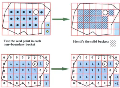
Identification of solid buckets

From the previous work on the distance transform, the algorithm has identified the boundary buckets and non-boundary buckets. Here for the purpose of efficiently searching the sub-region location of a query point with Cartesian coordinates, the method involves processing of all the non-boundary buckets in order to identify all the buckets that are inside the solid. For convenience we call such buckets 'solid buckets'. Figure 4-9 illustrates the algorithm.

The method for identifying the solid buckets involves assigning a sign to the digital distance value of each bucket. Solid buckets are non-boundary buckets, therefore, as long as one point inside a bucket is inside the solid, then the bucket is a solid bucket. So the algorithm is to use the center point of a non-boundary bucket as seed, check if this seed is inside the solid. If the seed is inside the solid then the corresponding bucket is a solid bucket, otherwise, the bucket is outside the solid. Therefore, the problem essentially 37

CHAPTER 4. PREPROCESSING OF FINITE ELEMENT FGM MODEL

Test the seed point in each non-boundary bucket

0 00 0 0 0 00

1 1 1 0 1 0 1 2 2 1 1 0 o -S0 '4 - 0 1

Identify the solid buckets

(

1 11 1

1

C

1 0

1

0 1 1 -1

Figure 4-9: Identify the signs of non-boundary buckets

becomes checking if a point is inside the solid, which will be explained in detail later together with the point location algorithm.

4.7 Bucketing vertices

After the bucketing processing of boundary facets, all the vertices of finite element mesh are also classified with respect to buckets, which will help the point classification queries of the model. Figure 4-10 illustrates the method, in which the white vertices are represen-tative vertices. The procedure is simply taking the integer parts of each vertex's bucket coordinates, and insert the vertex into the list of vertices of the corresponding bucket. For each bucket, the vertex that has the minimum number of parent tetrahedra is considered as the representative vertex of that bucket.

4 1 we W 0 41 **

0 1

Figure 4-10: Bucketing vertices based on the original bucket system

38

4

3

2 1